Introduction to Optimum Design phần 4 pdf
Bạn đang xem bản rút gọn của tài liệu. Xem và tải ngay bản đầy đủ của tài liệu tại đây (586.53 KB, 76 trang )
206 INTRODUCTION TO OPTIMUM DESIGN
TABLE 6-5 Pivot Step to Interchange Basic Variable x
4
with Nonbasic Variable x
l
for
Example 6.5
Initial canonical form.
BasicØ x
1
x
2
x
3
x
4
b
1 x
3
-11104
2 x
4
11016
Basic solution: Nonbasic variables: x
1
= 0, x
2
= 0
Basic variables: x
3
= 4, x
4
= 6
To interchange x
1
with x
4
, choose row 2 as the pivot row and column 1 as the pivot column.
Perform elimination using a
21
as the pivot element.
Result of the pivot operation: second canonical form.
BasicØ x
1
x
2
x
3
x
4
b
1 x
3
0 21110
2 x
1
1 101 6
Basic solution: Nonbasic variables: x
2
= 0, x
4
= 0
Basic variables: x
1
= 6, x
3
= 10
Solution. The given canonical form can be written in a tableau as shown in Table
6-5; x
1
and x
2
are nonbasic and x
3
and x
4
are basic, i.e., x
1
= x
2
= 0, x
3
= 4, x
4
.= 6. This
corresponds to point A in Fig. 6-2. In the tableau, the basic variables are identified in
the leftmost column and the rightmost column gives their values. Also, the basic vari-
ables can be identified by examining columns of the tableau. The variables associated
with the columns of the identity matrix are basic; e.g., variables x
3
and x
4
in Table 6-
5. Location of the positive unit element in a basic column identifies the row whose
right side parameter b
i
is the current value of the basic variable associated with that
column. For example, the basic column x
3
has unit element in the first row, and so x
3
is the basic variable associated with the first row. Similarly, x
4
is the basic variable
associated with row 2.
To make x
1
basic and x
4
a nonbasic variable, one would like to make a¢
21
= 1 and
a¢
11
= 0. This will replace x
1
with x
4
as the basic variable and a new canonical form
will be obtained. The second row is treated as the pivot row, i.e., a
21
= 1 (p = 2, q =
1) is the pivot element. Performing Gauss-Jordan elimination in the first column with
a
21
= 1 as the pivot element, we obtain the second canonical form as shown in Table
6-5. For this canonical form, x
2
= x
4
= 0 are the nonbasic variables and x
1
= 6 and x
3
= 10 are the basic variables. Thus, referring to Fig. 6-2, this pivot step results in a
move from the extreme point A(0, 0) to an adjacent extreme point D(6, 0).
6.3.5 Basic Steps of the Simplex Method
In this section, we shall illustrate the basic steps of the Simplex method with an example
problem. In the next subsection, we shall explain the basis for these steps and summarize
them in a step-by-step general algorithm. The method starts with a basic feasible solution,
i.e., at a vertex of the convex polyhedron. A move is then made to an adjacent vertex while
maintaining feasibility of the new solution as well as reducing the cost function. This is
accomplished by replacing a basic variable with a nonbasic variable. In the Simplex method,
movements are to the adjacent vertices only. Since there may be several points adjacent to
the current vertex, we naturally wish to choose the one that makes the greatest improvement
in the cost function f. If adjacent points make identical improvements in f, the choice becomes
arbitrary. An improvement at each step ensures no backtracking. Two basic questions now
arise:
1. How to choose a current nonbasic variable that should become basic?
2. Which variable from the current basic set should become nonbasic?
The Simplex method answers these questions based on some theoretical considerations
which shall be discussed in Chapter 7. Here, we consider an example to illustrate the basic
steps of the Simplex method that answer the foregoing two questions. Before presentation of
the example problem, an important requirement of the Simplex method is discussed. In this
method the cost function must always be given in terms of the nonbasic variables only. To
accomplish this, the cost function expression c
T
x = f is written as another linear equation in
the Simplex tableau; for example, the (m + l)th row. One then performs the pivot step on the
entire set of (m + 1) equations so that x
1
, x
2
, , x
m
and f are the basic variables. This way
the last row of the tableau representing the cost function expression is automatically given
in terms of the nonbasic variables after each pivot step. The coefficients in the nonbasic
columns of the last row are called the reduced cost coefficients written as c¢
j
. Example 6.6
describes the steps of the Simplex method in a systematic way.
Linear Programming Methods for Optimum Design 207
EXAMPLE 6.6 Steps of the Simplex Method
Solve the following LP problem: maximize
Solution. The graphical solution for the problem is given in Fig. 6-3. It can be seen
that the problem has an infinite number of solutions along the line C–D (z* = 4)
because the objective function is parallel to the second constraint. The Simplex method
is illustrated in the following steps:
1. Convert the problem to the standard form. We write the problem in the
standard LP form by transforming the maximization of z to minimization of
f =-2x
1
- x
2
, and adding slack variables x
3
, x
4
, and x
5
to the constraints. Thus,
the problem becomes
(a)
subject to
(b)
(c)
24
124
xxx++=
43 12
123
xxx++=
minimize fxx=- -2
12
zxx xx xx x x xx=+ +£ +£ +£ ≥2431224240
12 1 2 12 1 2 12
subject to ,,,
,
208 INTRODUCTION TO OPTIMUM DESIGN
4
2x
1
+ x
2
= 4
4x
1
+ 3x
2
= 12
x
1
+ 2x
2
= 4
4
3
3
2
2
1
10
A
B
C
D
F
E
Optimum solution line CD
x
2
x
1
G
z
* = 4
z = 2
z = 3
FIGURE 6-3 Graphical solution for the LP problem of Example 6.6. Optimum solution:
along line C–D. z* = 4.
(d)
(e)
We use the tableau and notation of Table 6-3 which will be augmented with
the cost function expression as the last row. The initial tableau for the
problem is shown in Table 6-6, where the cost function expression -2x
1
- x
2
= f is written as the last row. Note also that the cost function is in terms of
only the nonbasic variables x
1
and x
2
. This is one of the basic requirements of
the Simplex method—that the cost function always be in terms of the
nonbasic variables. When the cost function is only in terms of the nonbasic
variables, then the cost coefficients in the last row are the reduced cost
coefficients, written as c¢
j
.
2. Initial basic feasible solution.
To initiate the Simplex method, a basic feasible solution is needed. This is
already available in Table 6-6 which is given as:
basic variables: x
3
= 12, x
4
= 4, x
5
= 4
nonbasic variables: x
1
= 0, x
2
= 0
cost function: f = 0
Note that the cost row gives 0 = f after substituting for x
1
and x
2
. This
solution represents point A in Fig. 6-3 where none of the constraints is active
except the nonnegativity constraints on the variables.
3. Optimality check. We scan the cost row, which should have nonzero entries
only in the nonbasic columns, i.e., x
1
and x
2
. If all the nonzero entries are
nonnegative, then we have an optimum solution because the cost function
xi
i
≥=01; to 5
xxx
125
24++=
Linear Programming Methods for Optimum Design 209
cannot be reduced any further and the Simplex method is terminated. There
are negative entries in the cost row so the current basic feasible solution is
not optimum (see Chapter 7 for further explanation).
4. Choice of a nonbasic variable to become basic. We select a nonbasic column
having a negative cost coefficient; i.e., -2 in the x
1
column. This identifies a
nonbasic variable (x
1
) that should become basic. Thus, eliminations will be
performed in the x
1
column. This answers question 1 posed earlier: “How to
choose a current nonbasic variable that should become basic?” Note also that
when there is more than one negative entry in the cost row, the variable
tapped to become basic is arbitrary among the indicated possibilities. The
usual convention is to select a variable associated with the smallest value in
the cost row (or, negative element with the largest absolute value).
Notation. The boxed negative reduced cost coefficient in Table 6-6 indicates
the nonbasic variable associated with that column selected to become basic, a nota-
tion that is used throughout.
5. Selection of a basic variable to become nonbasic. To identify which current
basic variable should become nonbasic (i.e., to select the pivot row), we take
ratios of the right side parameters with the positive elements in the x
1
column
as shown in Table 6-7. We identify the row having the smallest positive ratio,
i.e., the second row. This will make x
4
nonbasic. The pivot element is a
21
= 2
(the intersection of pivot row and pivot column). This answers the question 2
posed earlier: “Which variable from the current basic set should become
nonbasic?” Selection of the row with the smallest ratio as the pivot row
maintains feasibility of the new basic solution. This is justified in Chapter 7.
TABLE 6-6 Initial Tableau for the LP Problem of Example 6.6
BasicØ x
1
x
2
x
3
x
4
x
5
b
1 x
3
4 310012
2 x
4
2 1010 4
3 x
5
1 2001 4
Cost function -2 -1 000f
Notation. The reduced cost coefficients in the nonbasic columns are boldfaced. The selected
negative reduced cost coefficient is boxed.
TABLE 6-7 Selection of Pivot Column and Pivot Row for Example 6.6
BasicØ x
1
x
2
x
3
x
4
x
5
b Ratio: b
i
/a
i1
;a
i1
> 0
1 x
3
4310012
12
–
4
= 3
2 x
4
21010 4
4
–
2
= 2 ¨ smallest
3 x
5
12001 4
4
–
1
= 4
Cost function -2 -1 000f
The selected pivot element is boxed. Selected pivot row and column are shaded. x
1
should
become basic (pivot column). x
4
row has the smallest ratio, and so x
4
should become nonbasic.
210 INTRODUCTION TO OPTIMUM DESIGN
Notation. The selected pivot element is also boxed, and the pivot column and
row are shaded throughout.
6. Pivot operation. We perform eliminations in column x
1
using row 2 as the
pivot row and Eqs. (6.15) to (6.17) to eliminate x
1
from rows 1, 3, and the
cost row as follows:
• divide row 2 by 2, the pivot element
• multiply new row 2 by 4 and subtract from row 1 to eliminate x
1
from row 1
• subtract new row 2 from row 3 to eliminate x
1
from row 3
• multiply new row 2 by 2 and add to the cost row to eliminate x
1
As a result of this elimination step, a new tableau is obtained as shown in
Table 6-8. The new basic feasible solution is given as
basic variables: x
3
= 4, x
1
= 2, x
5
= 2
nonbasic variables: x
2
= 0, x
4
= 0
cost function: 0 = f + 4, f =-4
7. This solution is identified as point D in Fig. 6-3. We see that the cost function
has been reduced from 0 to -4. All coefficients in the last row are
nonnegative so no further reduction of the cost function is possible. Thus, the
foregoing solution is the optimum. Note that for this example, only one
iteration of the Simplex method gave the optimum solution. In general, more
iterations are needed until all coefficients in the cost row become
nonnegative.
Note that the cost coefficients corresponding to the nonbasic variable x
2
in the last
row is zero in the final tableau. This is an indication of multiple solutions for the
problem. In general, when the reduced cost coefficient in the last row corresponding
to a nonbasic variable is zero, the problem may have multiple solutions. We shall
discuss this point later in more detail.
Let us see what happens if we do not select a row with the least ratio as the pivot
row. Let a
31
= 1 in the third row be the pivot element in Table 6-6. This will inter-
change nonbasic variable x
1
with the basic variable x
5
. Performing the elimination
steps in the first column as explained earlier, we obtain the new tableau given in Table
6-9. From the tableau, we have
basic variables: x
3
=-4, x
4
=-4, x
1
= 4
nonbasic variables: x
2
= 0, x
5
= 0
cost function: 0 = f + 8, f =-8
TABLE 6-8 Second Tableau for Example 6.6 Making x
1
a Basic Variable
BasicØ x
1
x
2
x
3
x
4
x
5
b
1 x
3
01 1 -204
2 x
1
1 0.5 0 0.5 0 2
3 x
5
0 1.5 0 -0.5 1 2
Cost function 0 0 0 1 0 f + 4
The cost coefficient in nonbasic columns are nonnegative; the tableau gives the optimum
solution.
Linear Programming Methods for Optimum Design 211
The foregoing solution corresponds to point G in Fig. 6-3. We see that this basic
solution is not feasible because x
3
and x
4
have negative values. Thus, we conclude that
if a row with the smallest ratio (of right sides with positive elements in the pivot
column) is not selected, the new basic solution is not feasible. Note that a spreadsheet
program, such as Excel, can be used to carry out the pivot step. Such a program can
facilitate learning of the Simplex method without getting bogged down with the
manual elimination process.
TABLE 6-9 Result of Improper Pivoting in Simplex Method for LP Problem of
Example 6.6
BasicØ x
1
x
2
x
3
x
4
x
5
b
1 x
3
0 -51 0 -4 -4
2 x
4
0 -30 1 -2 -4
3 x
1
1200 14
Cost function 0 3 00 4 f + 8
The pivot step making x
l
basic and x
5
nonbasic in Table 6-6 gives a basic solution that is not
feasible.
6.3.6 Simplex Algorithm
In the previous subsection, basic steps of the Simplex method are explained and illustrated
with an example problem. In this subsection, the underlying principles for these steps are
summarized in two theorems, called basic theorems of linear programming. We have seen
that in general the reduced cost coefficients c¢
j
of the nonbasic variables may be positive, neg-
ative, or zero. Let one of c¢
j
be negative, then if a positive value is assigned to the associated
nonbasic variable (i.e., it is made basic), the value of f will decrease. If more than one neg-
ative c¢
j
is present, a widely used rule of thumb is to choose the nonbasic variable associated
with the smallest c¢
j
(i.e., the most negative c¢
j
) to become basic. Thus, if any c¢
j
for (m + 1) £
j £ n (for nonbasic variables) is negative, then it is possible to find a new basic feasible solu-
tion (if one exists) that will further reduce the cost function. If a c¢
j
is zero, then the associ-
ated nonbasic variable can be made basic without affecting the cost function value. If all c¢
j
are nonnegative, then it is not possible to reduce the cost function any further, and the current
basic feasible solution is optimum. These ideas are summarized in the following Theorems
6.3 and 6.4.
Theorem 6.3 Improvement of Basic Feasible Solution Given a nondegenerate basic fea-
sible solution with the corresponding cost function f
0
, suppose that c¢
j
< 0 for some j. Then,
there is a feasible solution with f < f
0
. If the jth nonbasic column associated with c¢
j
can be
substituted for some column in the original basis, the new basic feasible solution will have
f < f
0
. If the jth column cannot be substituted to yield a basic feasible solution (i.e., there is
no positive element in the jth column), then the feasible set is unbounded and the cost func-
tion can be made arbitrarily small (toward negative infinity).
Theorem 6.4 Optimum Solution for LP Problems If a basic feasible solution has reduced
cost coefficients c¢
j
≥ 0 for all j, then it is optimum.
According to Theorem 6.3, the basic procedure of the Simplex method is to start with an
initial basic feasible solution, i.e., at the vertex of the convex polyhedron. If this solution is
not optimum according to Theorem 6.4, then a move is made to an adjacent vertex to reduce
the cost function. The procedure is continued until the optimum is reached. The steps of the
Simplex method illustrated in the previous subsection in Example 6.6 are summarized as
follows assuming that the initial tableau has been set up as described earlier:
Step 1. Initial Basic Feasible Solution This is readily obtained if all constraints are “£
type” because the slack variables can be selected as basic and the real variables as nonbasic.
If there are equality or “≥ type” constraints, then the two-phase simplex procedure explained
in the next section must be used.
Step 2. The Cost Function Must be in Terms of Only the Nonbasic Variables This is
readily available when there are only “£ type” constraints and slack variables are added into
them to convert the inequalities to equalities. The slack variables are basic, and they do not
appear in the cost function. In subsequent iterations, eliminations must also be performed in
the cost row.
Step 3. If All the Reduced Cost Coefficients for Nonbasic Variables Are Nonnegative
(≥0), We Have the Optimum Solution Otherwise, there is a possibility of improving the
cost function. We need to select a nonbasic variable that should become basic. We identify
a column having negative reduced cost coefficient because the nonbasic variable associated
with this column can become basic to reduce the cost function from its current value. This
is called the pivot column.
Step 4. If All Elements in the Pivot Column Are Negative, Then We Have an Unbounded
Problem Design problem formulation should be examined to correct the situation. If there
are positive elements in the pivot column, then we take ratios of the right side parameters with
the positive elements in the pivot column and identify a row with the smallest positive ratio. In
the case of a tie, any row among the tying ratios can be selected. The basic variable associated
with this row should become nonbasic (i.e., become zero). The selected row is called the pivot
row, and its intersection with the pivot column identifies the pivot element.
Step 5. Complete the Pivot Step Use the Gauss-Jordan elimination procedure and the
pivot row identified in Step 4. Elimination must also be performed in the cost function row
so that it is only in terms of nonbasic variables in the next tableau. This step eliminates the
nonbasic variable identified in Step 3 from all the rows except the pivot row.
Step 6. Identify Basic and Nonbasic Variables, and Their Values Identify the cost func-
tion value and go to Step 3.
Note that when all the reduced cost coefficient c¢
j
in the nonbasic columns are strictly pos-
itive, the optimum solution is unique. If at least one c¢
j
is zero in a nonbasic column, then
there is a possibility of an alternate optimum. If the nonbasic variable associated with a zero
reduced cost coefficient can be made basic by using the foregoing procedure, the extreme
point (vertex) corresponding to an alternate optimum is obtained. Since the reduced cost coef-
ficient is zero, the optimum cost function value will not change. Any point on the line segment
joining the optimum extreme points also corresponds to an optimum. Note that all these
optima are global as opposed to local, although there is no distinct global optimum. Geo-
metrically, multiple optima for an LP problem imply that the cost function hyperplane is par-
allel to one of the constraint hyperplanes. Example 6.7 shows how to obtain a solution for
an LP problem using the Simplex method.
212 INTRODUCTION TO OPTIMUM DESIGN
Linear Programming Methods for Optimum Design 213
EXAMPLE 6.7 Solution by the Simplex Method
Using the Simplex method, find the optimum (if one exists) for the LP problem of
Example 6.3:
(a)
subject to
(b)
(c)
(d)
Solution. Writing the problem in the Simplex tableau, we obtain the initial canoni-
cal form as shown in Table 6-10. From the initial tableau, the basic feasible solution
is
Note that the cost function in the last row is in terms of only nonbasic variables x
1
and x
2
. Thus, coefficients in the x
1
and x
2
columns and the last row are the reduced
cost function: f = 0 from the last row of the tableau
nonbasic variables: xx
12
0==
basic variables: xx
34
46==,
xi
i
≥=01; to 4
xxx
124
6++=
-+ + =xxx
123
4
minimize fxx=- -45
12
TABLE 6-10 Solution of Example 6.7 by the Simplex Method
Initial tableau: x
3
is identified to be replaced with x
2
in the basic set.
BasicØ x
1
x
2
x
3
x
4
b Ratio: b
i
/a
iq
x
3
-1110 4
4
–
1
= 4 ¨ smallest
x
4
1101 6
6
–
1
= 6
Cost -4 -5 00 f
Second tableau: x
4
is identified to be replaced with x
1
in the basic
set.
BasicØ x
1
x
2
x
3
x
4
b Ratio: b
i
/a
iq
x
2
-1 1 1 0 4 Negative
x
4
2 0 -11 2
2
–
2
= 1
Cost -9 0 5 0 f + 20
Third tableau: Reduced cost coefficients in nonbasic columns are
nonnegative; the tableau gives optimum point.
BasicØ x
1
x
2
x
3
x
4
b Ratio: b
i
/a
iq
x
2
01
1
–
2
1
–
2
5 Not needed
x
1
10-
1
–
2
1
–
2
1 Not needed
Cost 0 0
1
–
2
9
–
2
f + 29
Example 6.8 demonstrates the solution of the profit maximization problem by the Simplex
method.
214 INTRODUCTION TO OPTIMUM DESIGN
cost coefficients c¢
j
. Scanning the last row, we observe that there are negative coeffi-
cients. Therefore, the current basic solution is not optimum. In the last row, the most
negative coefficient of -5 corresponds to the second column. Therefore, we select x
2
to become a basic variable, i.e., elimination should be performed in the x
2
column.
This fixes the column index q to 2 in Eq. (6.15). Now taking the ratios of the right
side parameters with positive coefficients in the second column b
i
/a
i2
, we obtain a
minimum ratio for the first row as 4. This identifies the first row as the pivot row
according to Step 4. Therefore, the current basic variable associated with the first row,
x
3
, should become nonbasic. Now performing the pivot step on column 2 with a
12
as
the pivot element, we obtain the second canonical form (tableau) as shown in Table
6-10. For this canonical form the basic feasible solution is
The cost function is f =-20 (0 = f + 20), which is an improvement from f = 0.
Thus, this pivot step results in a move from (0, 0) to (0, 4) on the convex polyhedron
of Fig. 6-2.
The reduced cost coefficient corresponding to the nonbasic column x
1
is negative.
Therefore, the cost function can be reduced further. Repeating the above-mentioned
process for the second tableau, we obtain a
21
= 2 as the pivot element, implying that
x
1
should become basic and x
4
should become nonbasic. The third canonical form is
shown in Table 6-10. For this tableau, all the reduced cost coefficients c¢
j
(corre-
sponding to the nonbasic variables) in the last row are ≥0. Therefore, the tableau yields
the optimum solution as x
1
= 1, x
2
= 5, x
3
= 0, x
4
= 0, f =-29 (f + 29 = 0), which cor-
responds to the point C (1,5) in Fig. 6-2.
nonbasic variables: xx
13
0==
basic variables: xx
24
42==,
EXAMPLE 6.8 Solution of Profit Maximization Problem by
the Simplex Method
Use the Simplex method to find the optimum solution for the profit maximization
problem of Example 6.2.
Solution. Introducing slack variables in the constraints of Eqs. (c) through (e) in
Example 6.2, we get the LP problem in the standard form:
(a)
subject to
(b)
(c)
1
28
1
14
1
124
xxx++=
xxx
123
16++=
minimize fxx=- -400 600
12
Linear Programming Methods for Optimum Design 215
(d)
(e)
Now writing the problem in the standard Simplex tableau, we obtain the initial
canonical form as shown in Table 6-11. Thus the initial basic feasible solution is x
1
=
0, x
2
= 0, x
3
= 16, x
4
= x
5
= 1, f = 0, which corresponds to point A in Fig. 6-1. The
initial cost function is zero, and x
3
, x
4
, and x
5
are the basic variables.
Using the Simplex procedure, we note thata
22
=
1
–
14
is the pivot element. This implies
that x
4
should be replaced by x
2
in the basic set. Carrying out the pivot operation using
the second row as the pivot row, we obtain the second tableau (canonical form) shown
in Table 6-11. At this point the basic feasible solution is x
1
= 0, x
2
= 14, x
3
= 2, x
4
=
0, x
5
=
5
–
12
, which corresponds to point E in Fig. 6-1. The cost function is reduced to
-8400. The pivot element for the next step is a
11
, implying that x
3
should be replaced
by x
1
in the basic set. Carrying out the pivot operation, we obtain the third canonical
form shown in Table 6-11. At this point all reduced cost coefficients (corresponding
to nonbasic variables) are nonnegative, so according to Theorem 6.4, we have the
optimum solution: x
1
= 4, x
2
= 12, x
3
= 0, x
5
=
3
–
14
. This corresponds to the D in
xi
i
≥=01; to 5
1
14
1
24
1
125
xxx++=
TABLE 6-11 Solution of Example 6.8 by the Simplex Method
Initial tableau: x
4
is identified to be replaced with x
2
in the basic set.
BasicØ x
1
x
2
x
3
x
4
x
5
b Ratio: b
i
/a
iq
x
3
1110016
16
–
1
= 16
x
4
1
–
28
1
–
14
01 01
1
—
1/14
= 14 ¨ smallest
x
5
1
–
14
1
–
24
00 11
1
—
1/24
= 24
Cost -400 -600 00 0f - 0
Second tableau: x
3
is identified to be replaced with x
1
in the basic
set.
BasicØ x
1
x
2
x
3
x
4
x
5
b Ratio: b
i
/a
iq
x
3
1
–
2
01-14 0 2
2
—
1/2
= 4 ¨ smallest
x
2
1
–
2
1 0 14 0 14
14
—
1/2
= 28
x
5
17
—
336
00 -
7
–
12
1
5
–
12
5/12
—
17/336
=
140
—
17
Cost -100 008400 0 f + 8400
Third tableau: Reduced cost coefficients in the nonbasic columns are
nonnegative; the tableau gives optimum solution
BasicØ x
1
x
2
x
3
x
4
x
5
b Ratio: b
i
/a
iq
x
3
10 2-28 0 4 Not needed
x
2
01 -1 28 0 12 Not needed
x
5
00-
17
—
168
5
–
6
1
3
–
14
Not needed
Cost 0 0 200 5600 0 f + 8800
216 INTRODUCTION TO OPTIMUM DESIGN
Fig. 6-1. The optimum value of the cost function is -8800. Note that c¢
j
, correspond-
ing to the nonbasic variables x
3
and x
4
, are positive. Therefore, the global optimum is
unique, as may be observed in Fig. 6-1 as well.
EXAMPLE 6.9 LP Problem with Multiple Solutions
Solve the following problem by the Simplex method: maximize z = x
1
+ 0.5x
2
subject
to 2x
1
+ 3x
2
£ 12, 2x
1
+ x
2
£ 8, x
1
, x
2
≥ 0.
Solution. The problem was solved graphically in Section 3.4 of Chapter 3. It has
multiple solutions as may be seen in Fig. 3-7. We will solve the problem using the
Simplex method and discuss how multiple solutions can be recognized for genera1
LP problems. The problem is converted to standard LP form:
(a)
subject to
(b)
(c)
(d)
Table 6-12 contains iterations of the Simplex method. The optimum point is reached
in just one iteration because all the reduced cost coefficients are nonnegative in the
second canonical form (second tableau). The solution is given as
basic variables: x
1
= 4, x
3
= 4
nonbasic variables: x
2
= x
4
= 0
optimum cost function: f =-4
The solution corresponds to point B in Fig. 3-7. In the second tableau, the reduced
cost coefficient for the nonbasic variable x
2
is zero. This means that it is possible to
make x
2
basic without any change in the optimum cost function value. This suggests
existence of multiple optimum solutions. Performing the pivot operation in column 2,
we find another solution given in the third tableau of Table 6-12 as:
basic variables: x
1
= 3, x
2
= 2
nonbasic variables: x
3
= x
4
= 0
optimum cost function: f =-4
xi
i
≥=01; to 4
28
124
xxx++=
23 12
123
xxx++=
minimize fx x=- -
12
05.
Problem in Example 6.9 has multiple solution. The example illustrates how to recognize
such solutions with the Simplex method.
Linear Programming Methods for Optimum Design 217
This solution corresponds to point C on Fig. 3-7. Note that any point on the line B–C
also gives an optimum solution. Multiple solutions can occur when the cost function
is parallel to one of the constraints. For the present example, the cost function is par-
allel to the second constraint, which is active at the solution.
TABLE 6-12 Solution by the Simplex Method for Example 6.9
Initial tableau: x
4
is identified to be replaced with x
1
in the basic set.
BasicØ x
1
x
2
x
3
x
4
b Ratio: b
i
/a
iq
x
3
23 1012
12
–
2
= 6
x
4
21 018
8
–
2
= 4 ¨ smallest
Cost -1 -0.5 00f - 0
Second tableau: First optimum point; reduced cost coefficients in
nonbasic columns are nonnegative; the tableau gives optimum
solution. c¢
3
= 0 indicates the possibility of multiple solutions. x
3
is
identified to be replaced with x
2
in the basic set to obtain another
optimum point.
BasicØ x
1
x
2
x
3
x
4
b Ratio: b
i
/a
iq
x
3
02 1-14
4
–
2
= 2 ¨ smallest
x
1
1
1
–
2
0
1
–
2
4
4
—
1/2
= 8
Cost 0 0 0
1
–
2
f + 4
Third tableau: Second optimum point.
BasicØ x
1
x
2
x
3
x
4
b Ratio: b
i
/a
iq
x
2
01
1
–
2
-
1
–
2
2 Not needed
x
1
10 -
1
–
4
3
–
4
3 Not needed
Cost 0 0 0
1
–
2
f + 4
In general, if a reduced cost coefficient corresponding to a nonbasic variable is zero in
the final tableau, there is a possibility of multiple optimum solutions. From a practical stand-
point, this is not a bad situation. Actually, it may be desirable because it gives the designer
options; any suitable point on the straight line joining the two optimum designs can be
selected to better suit the needs of the designer. Note that all optimum design points are global
solutions as opposed to local solutions.
Example 6.10 demonstrates how to recognize an unbounded feasible set (solution) for a
problem.
218 INTRODUCTION TO OPTIMUM DESIGN
EXAMPLE 6.10 Identification of an Unbounded Problem
with the Simplex Method
Solve the LP problem: maximize z = x
1
- 2x
2
subject to 2x
1
- x
2
≥ 0, -2x
1
+ 3x
2
£ 6,
x
1
, x
2
≥ 0
Solution. The problem has been solved graphically in Section 3.5. It can be seen
from the graphical solution (Fig. 3-8) that the problem is unbounded. We will solve
the problem using the Simplex method and see how we can recognize unbounded
problems. Writing the problem in the standard Simplex form, we obtain the initial
canonical form shown in Table 6-13 where x
3
and x
4
are the slack variables (note that
the first constraint has been transformed as -2x
1
+ x
2
£ 0). The basic feasible solution
is
basic variables: x
3
= 0, x
4
= 5
nonbasic variables: x
1
= x
2
= 0
cost function: f = 0
TABLE 6-13 Initial Canonical form for Example 6.10 (Unbounded Problem)
BasicØ x
1
x
2
x
3
x
4
b
x
3
-21 10 0
x
4
-23 01 6
Cost -12 00 f - 0
Scanning the last row, we find that the reduced cost coefficient for the nonbasic vari-
able x
1
is negative. Therefore, x
1
should become a basic variable. However, a pivot
element cannot be selected in the first column because there is no positive element.
There is no other possibility of selecting another nonbasic variable to become basic;
the reduced cost coefficient for x
2
(the other nonbasic variable) is positive. Therefore,
no pivot steps can be performed, and yet we are not at the optimum point. Thus, the
feasible set for the problem is unbounded. The foregoing observation will be true in
general. For unbounded problems, there will be negative reduced cost coefficients for
nonbasic variables but no possibility of pivot steps.
6.4 Two-Phase Simplex Method—Artificial Variables
The basic Simplex method of Section 6.3 is extended to handle “≥ type” and equality con-
straints. A basic feasible solution is needed to initiate the Simplex solution process. Such a
solution is immediately available if only “£ type” constraints are present. However, for the
“≥ type” and equality constraints, an initial basic feasible solution is not available. To obtain
such a solution, we must introduce artificial variables for the “≥ type” and equality con-
straints, define an auxiliary minimization LP problem, and solve it. The standard Simplex
method can still be used to solve the auxiliary problem. This is called Phase I of the Simplex
procedure. At the end of Phase I, a basic feasible solution for the original problem becomes
available. Phase II then continues to find a solution to the original LP problem. The method
is illustrated with examples.
6.4.1 Artificial Variables
When there are “≥ type” constraints in the LP problem, surplus variables are subtracted from
them to transform the problem to the standard form. The equality constraints, if present, are
not changed because they are already in the standard form. For such problems, an initial basic
solution cannot be obtained by selecting the original design variables as nonbasic (setting
them to zero), as is the case when there are only “£ type” constraints, e.g., for all the exam-
ples in Section 6.3. To obtain an initial basic feasible solution, the Gauss-Jordan elimination
procedure can be used to convert the Ax = b in the canonical form. However, an easier way
is to introduce nonnegative auxiliary variables for the “≥ type” and equality constraints, define
an auxiliary LP problem, and solve it using the Simplex method. The auxiliary variables are
called artificial variables and are different from the surplus variables. They have no physi-
cal meaning; however, with their addition we obtain an initial basic feasible solution for the
auxiliary LP problem by treating them as basic along with any slack variables for “£ type”
constraints. All other variables are treated as nonbasic (i.e., set to zero).
For the sake of simplicity of discussion, let us assume that each constraint of the standard
LP problem requires an artificial variable. We shall see later in examples that constraints that
do not require an artificial variable can also be treated routinely. Recalling that the standard
LP problem has n variables and m constraints, the constraint equations augmented with the
artificial variables are written as
(6.18)
where x
n+j
, j = 1 to m are the artificial variables. The constraints of Eq. (6.18) can be written
in the summation notation as
(6.19)
Thus the initial basic feasible solution is obtained as x
j
= 0, j = 1 to n, and x
n+i
= b
i
, i = 1
to m. Note that the artificial variables basically augment the convex polyhedron of the
original problem. The initial basic feasible solution corresponds to an extreme point (vertex)
located in the new expanded space. The problem now is to traverse extreme points in the
expanded space until an extreme point is reached in the original space. When the original
space is reached, all artificial variables will be nonbasic (i.e., they will have zero value). At
this point the augmented space is literally removed so that future movements are only among
the extreme points of the original space until the optimum is reached. In short, after creating
artificial variables, we eliminate them as quickly as possible. The preceding procedure is
called the two-phase Simplex method of LP.
6.4.2 Artificial Cost Function
To eliminate the artificial variables from the problem, we define an auxiliary function called
the artificial cost function, and minimize it subject to the constraints of Eq. (6.19) and non-
negativity of all the variables. The artificial cost function is simply a sum of all the artificial
variables and will be designated as w:
ax x b i m
ij j n i
j
n
i
+= =
+
=
Â
1
1; to
ax ax ax x b
ax ax ax x b
nn n
mm mnnnmm
11 1 12 2 1 1 1
11 22
++++=
++++=
+
+
. . . .
. . . .
Linear Programming Methods for Optimum Design 219
(6.20)
6.4.3 Definition of Phase I Problem
Since the artificial variables are introduced to simply obtain an initial basic feasible solution
for the original problem, they need to be eliminated eventually. This elimination is done by
defining an LP problem called the Phase I problem. The objective of this problem is to make
all the artificial variables nonbasic so that they have zero value. In that case, the artificial cost
function in Eq. (6.20) will be zero, indicating the end of Phase I. However the Phase I problem
is not yet in a form suitable to initiate the Simplex method. The reason is that the reduced
cost coefficients c¢
j
of the nonbasic variables in the artificial cost function are not yet avail-
able to determine the pivot element and perform the pivot step. Currently, the artificial cost
function in Eq. (6.20) is in terms of the basic variables x
n+1
, , x
n+m
. Therefore the reduced
cost coefficients c¢
j
cannot be identified. They can be identified only if the artificial cost func-
tion w is in terms of the nonbasic variables x
1
, , x
n
. To obtain w in terms of nonbasic vari-
ables, we use the constraint expressions to eliminate the basic variables from the artificial
cost function. Calculating x
n+1
, , x
n+m
from Eqs. (6.18) and substituting into Eq. (6.20), we
obtain the artificial cost function w in terms of the nonbasic variables as
(6.21)
The reduced cost coefficients c¢
j
are identified as the coefficients of the nonbasic variables x
j
in Eq. (6.21) as
(6.22)
If there are also “£ type” constraints in the original problem, these are cast into the stan-
dard LP form by adding slack variables that serve as basic variables in Phase I. Therefore,
the number of artificial variables is less than m—the total number of constraints. Accordingly,
the number of artificial variables required to obtain an initial basic feasible solution is also
less than m. This implies that the sums in Eqs. (6.21) and (6.22) are not for all the m con-
straints. They are only over the constraints requiring an artificial variable.
6.4.4 Phase I Algorithm
The standard Simplex procedure described in Section 6.3 can now be employed to solve the
auxiliary optimization problem of Phase I. During this phase, the artificial cost function is
used to determine the pivot element. The original cost function is treated as a constraint and
the elimination step is also executed for it. This way, the real cost function is in terms of the
nonbasic variables only at the end of Phase I, and the Simplex method can be continued
during Phase II. All artificial variables become nonbasic at the end of Phase I. Since w is the
sum of all the artificial variables, its minimum value is clearly zero. When w = 0, an extreme
point of the original feasible set is reached. w is then discarded in favor of f and iterations
continue in Phase II until the minimum of f is obtained. Suppose, however, that w cannot
be driven to zero. This will be apparent when none of the reduced cost coefficients for the
artificial cost function is negative and yet w is greater than zero. Clearly, this means that we
cannot reach the original feasible set and, therefore, no feasible solution exists for the
original design problem, i.e., it is an infeasible problem. At this point the designer should
re-examine the formulation of the problem, which may be over-constrained or improperly
formulated.
¢=- =
=
Â
cajn
jij
i
m
; 1
1
to
wb ax
iijj
i
m
j
n
i
m
=-
===
ÂÂÂ
111
wx x x x
nn nm ni
i
m
=+++ =
++ + +
=
Â
12
1
220 INTRODUCTION TO OPTIMUM DESIGN
6.4.5 Phase II Algorithm
In the final tableau from Phase I, the artificial cost row is replaced by the actual cost func-
tion equation and the Simplex iterations continue based on the algorithm explained in Section
6.3. The basic variables, however, should not appear in the cost function. Thus, pivot steps
need to be performed on the cost function equation to eliminate the basic variables from it.
A convenient way of accomplishing this is to treat the cost function as one of the equations
in the Phase I tableau, say the second equation from the bottom. Elimination is performed
on this equation along with others. In this way, the cost function is in the correct form to
continue with Phase II. The artificial variable columns can also be discarded for Phase II cal-
culations. However, they are kept in the tableau because they provide information that can
be useful for postoptimality analysis.
For most LP problems, the Simplex method yields one of the following results as illus-
trated in the examples:
1. If there is a solution to the problem, the method will find it (Example 6.11).
2. If the problem is infeasible, the method will indicate that (Example 6.12).
3. If the problem is unbounded, the method will indicate that (Example 6.10, Example
6.13).
4. If there are multiple solutions, the method will indicate that, as seen in Examples 6.6
and 6.9.
Linear Programming Methods for Optimum Design 221
EXAMPLE 6.11 Use of Artificial Variable for
“≥ Type” Constraints
Find the optimum solution for the following LP problem using the Simplex method:
maximize z = y
1
+ 2y
2
subject to 3y
1
+ 2y
2
£ 12, 2y
1
+ 3y
2
≥ 6, y
1
≥ 0, y
2
is unrestricted
in sign.
Solution. The graphical solution for the problem is shown in Fig. 6-4. It can be seen
that the optimum solution is at point B. We shall use the two-phase Simplex method
to verify the solution. Since y
2
is free in sign, we decompose it as y
2
= y
+
2
- y
-
2
. To
write the problem in the standard form, we define x
1
= y
1
, x
2
= y
+
2
, and x
3
= y
-
2
, and
transform the problem as
(a)
subject to
(b)
(c)
(d)
where x
4
is a slack variable for the first constraint and x
5
is a surplus variable for the
second constraint. It can be seen that if we select the real variables as nonbasic, i.e.,
x
1
= 0, x
2
= 0, x
3
= 0, the resulting basic solution is infeasible because x
5
=-6. There-
fore, we need to use the two-phase algorithm. Accordingly, we introduce an artificial
variable x
6
in the second constraint as
xi
i
≥=01; to 5
233 6
1235
xxxx+ =
32 2 12
1234
xxxx+-+=
minimize fxxx=- - +
123
22
222 INTRODUCTION TO OPTIMUM DESIGN
(e)
The artificial cost function is defined as w = x
6
. Since w should be in terms of non-
basic variables (x
6
is basic), we substitute for x
6
from Eq. (e) and obtain w as
(f)
The initial tableau for Phase I is shown in Table 6-14. The initial basic variables
are x
4
= 12 and x
6
= 6. The nonbasic variables are x
1
= x
2
= x
3
= x
5
= 0. Also w = 6
and f = 0. This corresponds to the infeasible point D in Fig. 6-4. According to the
Simplex algorithm, the pivot element is a
22
, which implies that x
2
should become basic
and x
6
should become nonbasic. Performing the pivot step, we obtain the second
tableau given in Table 6-14. For the second tableau, x
4
= 8 and x
2
= 2 are the basic
variables and all others are nonbasic. This corresponds to the feasible point A in Fig.
6-4. Since all the reduced cost coefficients of the artificial cost function are nonneg-
ative and the artificial cost function is zero, an initial basic feasible solution for the
original problem is obtained. Therefore, this is the end of Phase I.
For Phase II, column x
6
should be ignored in determining pivots. For the next step,
the pivot element is a
15
in the second tableau according to Steps 1 and 2 of the Simplex
method. This implies that x
4
should be replaced by x
5
as a basic variable. The third
tableau is obtained as shown in Table 6-14. The last tableau yields an optimum solu-
tion for the problem, which is x
5
= 12, x
2
= 6, x
1
= x
3
= x
4
= 0, and f =-12. The solu-
tion for the original design problem is then y
1
= 0, y
2
= 6, and z = 12, which agrees
with the graphical solution of Fig. 6-4. Note that the artificial variable column (x
6
) in
the final tableau is the negative of the surplus variable column (x
5
). This is true for all
“≥ type” constraints.
wx x x x x==- - + +
61235
62 3 3
233 6
12356
xxxxx+ +=
3y
1
+ 2y
2
= 12
2y
1
+ 3y
2
= 6
z = 10
z = 6
z = 2
4
4
6
6
2
2
0
A
B
C
D
Optimum point
y
2
y
1
y
1
= 0, y
2
= 6, z * = 12
FIGURE 6-4 Graphical solution for Example 6.11.
Linear Programming Methods for Optimum Design 223
TABLE 6-14 Solution by the Two-Phase Simplex Method for Example 6.11
Initial tableau: x
6
is identified to be replaced with x
2
in the basic set.
BasicØ x
1
x
2
x
3
x
4
x
5
x
6
b Ratio
x
4
32-210012
12
–
2
= 6
x
6
23-30 -11 6
6
–
3
= 2
Cost -1 -2200 0f - 0
Artificial cost -2 -330 1 0 w - 6
Second tableau: End of Phase I. Begin Phase II. x
4
is identified to be
replaced with x
5
in the basic set.
BasicØ x
1
x
2
x
3
x
4
x
5
x
6
b Ratio
x
4
5
–
3
001
2
–
3
-
2
–
3
8
8
—
2/3
= 12
x
2
2
–
3
1 -10 -
1
–
3
1
–
3
2 Negative
Cost
1
–
3
000-
2
–
3
2
–
3
f + 4
Artificial cost 0 0 0 0 01w - 0
Third tableau: Reduced cost coefficients in nonbasic columns are
nonnegative; the third tableau gives the optimum solution. End of
Phase II.
BasicØ x
1
x
2
x
3
x
4
x
5
x
6
b
x
5
5
–
2
00
3
–
2
1 -112
x
2
3
–
2
1 -1
1
–
2
006
Cost 2 001 00f + 12
EXAMPLE 6.12 Use of Artificial Variables for Equality
Constraints (Infeasible Problem)
Solve the LP problem: maximize z = x
1
+ 4x
2
subject to x
1
+ 2x
2
£ 5, 2x
1
+ x
2
= 4,
x
1
- x
2
≥ 3, x
1
, x
2
≥ 0.
Solution. The constraints for the problem are plotted in Fig. 6-5. It can be seen that
the problem has no feasible solution. We will solve the problem using the Simplex
method to see how we can recognize an infeasible problem. Writing the problem in
the standard LP form, we obtain
(a)
subject to
(b)
(c)
(d)
(e)
xi
i
≥=01; to 6
xxxx
1246
3 +=
24
125
xxx++=
xxx
123
25++=
minimize fxx=- -
12
4
224 INTRODUCTION TO OPTIMUM DESIGN
4
2x
1
+ x
2
= 4
x
1
+ 2x
2
=
5
x
1
– x
2
= 3
45
3
3
2
2
1
10
A
G
B
C
D
E
x
2
x
1
F
H
FIGURE 6-5 Constraints for Example 6.12. Infeasible problem.
TABLE 6-15 Solution for Example 6.12 (Infeasible Problem)
Initial tableau: x
5
is identified to be replaced with x
1
in the basic set.
BasicØ x
1
x
2
x
3
x
4
x
5
x
6
b Ratio
x
3
121 0005
5
–
1
= 5
x
5
210 0104
4
–
2
= 2
x
6
1 -10 -1013
3
–
1
= 3
Cost -1 -40 00 0 f - 0
Artificial cost -3 00 1 00w - 7
Second tableau: End of Phase I.
BasicØ x
1
x
2
x
3
x
4
x
5
x
6
b
x
3
0
3
–
2
10-
1
–
2
03
x
1
1
1
–
2
00
1
–
2
02
x
6
0 -
3
–
2
0 -1 -
1
–
2
11
Cost 0 -
7
–
2
00
1
–
2
0 f + 2
Artificial cost 0
3
–
2
0 1
3
–
2
0 w - 1
Here x
3
is a slack variable, x
4
is a surplus variable, and x
5
and x
6
are artificial vari-
ables. Table 6-15 shows Phase I iterations of the Simplex method. It can be seen that
after the first pivot step, all the reduced cost coefficients of the artificial cost function
for nonbasic variables are positive indicating the end of Phase I. However, the artifi-
cial cost function is not zero (w = 1). Therefore there is no feasible solution to the
original problem.
Linear Programming Methods for Optimum Design 225
EXAMPLE 6.13 Use of Artificial Variables (Unbounded
Problem)
Solve the LP problem: maximize z = 3x
1
- 2x
2
subject to x
1
- x
2
≥ 0, x
1
+ x
2
≥ 2,
x
1
, x
2
≥ 0.
Solution. The constraints for the problem are plotted in Fig. 6-6. It can be seen that
the problem is unbounded. We will solve the problem by the Simplex method and see
how to recognize unboundedness. Transforming the problem to the standard form, we
get:
(a)
subject to
(b)
(c)
(d)
where x
3
is a slack variable, x
4
is a surplus variable, and x
5
is an artificial variable.
Note that the right side of the first constraint is zero so it can be treated as either
“£ type” or “≥ type.” We will treat it as “£ type.” Note also that the second constraint
is “≥ type,” so we must use an artificial variable and an artificial cost function to find
the initial basic feasible solution. The solution for the problem is given in Table 6-16.
For the initial tableau x
3
= 0 and x
5
= 2 are basic variables and all others are nonba-
sic. Note that this is a degenerate basic feasible solution. The solution corresponds to
point A (the origin) in Fig. 6-6. Scanning the artificial cost row, we observe that there
are two possibilities for pivot columns, x
1
or x
2
. If x
2
is selected as the pivot column,
xi
i
≥=01; to 5
xxxx
1245
2
+-+=
-+ + =xxx
123
0
minimize fxx=- +32
12
x
1
+ x
2
= 2
x
1
+ x
2
= 0
3
3
2
2
1
10
A
B
C
D
Feasible region unbounded
x
2
x
1
FIGURE 6-6 Constraints for Example 6.13. Unbounded problem.
226 INTRODUCTION TO OPTIMUM DESIGN
then the first row must be the pivot row with a
12
= 1 as the pivot element. This will
make x
2
basic and x
3
nonbasic. However, x
2
will remain zero and the resulting solu-
tion will be degenerate, corresponding to point A. One more iteration will be neces-
sary to move from A to D. If we choose x
1
as the pivot column, then a
21
= 1 will be
the pivot element making x
1
as basic and x
5
as nonbasic. Carrying out the pivot step,
we obtain the second tableau as shown in Table 6-16. The basic feasible solution is
x
1
= 2, x
3
= 2, and other variables are zero. This solution corresponds to point D in
Fig. 6-6. This is the basic feasible solution for the original problem because the arti-
ficial cost function is zero, i.e., w = 0. The original cost function has also reduced
from 0 to -6. This is the end of Phase I. Scanning the cost function row, we find that
the reduced cost coefficient c¢
4
is negative, but the pivot element cannot be determined,
i.e., x
4
cannot be made basic (all elements in the x
4
column are negative in the second
tableau). This indicates the problem to be unbounded.
TABLE 6-16 Solution for Example 6.13 (Unbounded Problem)
Initial tableau: x
5
is identified to be replaced with x
1
in the basic set.
BasicØ x
1
x
2
x
3
x
4
x
5
b Ratio
x
3
-1 1 1 0 0 0 Negative
x
5
110-11 2
2
–
1
= 2
Cost -320 00f - 0
Artificial cost -1 -1 0 1 0 w - 2
Second tableau: End of Phase I. End of Phase II.
BasicØ x
1
x
2
x
3
x
4
x
5
b Ratio
x
3
02 1 -1 1 2 Negative
x
1
11 0 -1 1 2 Negative
Cost 0 5 0 -33 f + 6
Artificial cost 0 0 0 0 1 w - 0
6.4.6 Degenerate Basic Feasible Solution
It is possible that during iterations of the Simplex method, a basic variable attains zero value,
i.e., the basic feasible solution becomes degenerate. What are the implications of this situa-
tion? We shall discuss them in Example 6.14.
EXAMPLE 6.14 Implications of Degenerate Basic
Feasible Solution
Solve the following LP problem by the Simplex method: maximize z = x
1
+ 4x
2
subject
to x
1
+ 2x
2
£ 5, 2x
1
+ x
2
£ 4, 2x
1
+ x
2
≥ 4, x
1
- x
2
≥ 1, x
1
, x
2
≥ 0.
Solution. The problem is transcribed into the standard LP form as follows:
Linear Programming Methods for Optimum Design 227
(a)
subject to
(b)
(c)
(d)
(e)
(f)
where x
3
and x
4
are slack variables, x
5
and x
6
are surplus variables, and x
7
and x
8
are
artificial variables. The two-phase Simplex procedure takes three iterations to reach
the optimum point. These iterations are given in Table 6-17. It can be seen that in the
third tableau, the basic variable x
4
has zero value so the basic feasible solution is
degenerate. At this iteration, it is determined that x
5
should become basic so x
5
is the
pivot column. We need to determine the pivot row. We take ratios of the right sides
with the positive elements in the x
5
column. This determines the second row as the
pivot row because it has the lowest ratio (zero). In general, if the element in the pivot
column and the row that gives degenerate basic variable is positive, then that row must
always be the pivot row; otherwise, the new solution cannot be feasible. Also, in this
case, the new basic feasible solution will be degenerate, as for the final tableau in
Table 6-17. The only way the new feasible solution can be nondegenerate is when the
element in the pivot column and the degenerate variable row is negative. In that case
xi
i
≥=01; to 8
xxxx
1268
1 +=
24
1257
xxxx+-+=
24
124
xxx++=
xxx
123
25++=
minimize fxx=- -
12
4
TABLE 6-17 Solution for Example 6.14 (Degenerate Basic Feasible Solution)
Initial tableau: x
8
is identified to be replaced with x
1
in the basic set.
BasicØ x
1
x
2
x
3
x
4
x
5
x
6
x
7
x
8
b Ratio
x
3
1210 00005
5
–
1
= 5
x
4
2101 00004
4
–
2
= 2
x
7
2100-10104
4
–
2
= 2
x
8
1 -10 0 0-1011
1
–
1
= 1
Cost -1 -40 0 0 00 0 f - 0
Artificial -3 000 1100w - 5
Second tableau: x
7
is identified to be replaced with x
2
in the basic
set.
BasicØ x
1
x
2
x
3
x
4
x
5
x
6
x
7
x
8
b Ratio
x
3
0 310 010-14
4
–
3
x
4
0 301 020-22
2
–
3
x
7
0300-121-22
2
–
3
x
1
1 -10 0 0-1 0 1 1 Negative
Cost 0 -50 0 0-10 1f + 1
Artificial 0 -3 00 1 -2 0 3 w - 2
228 INTRODUCTION TO OPTIMUM DESIGN
TABLE 6-17 Continued
Third tableau: x
4
is identified to be replaced with x
5
in the basic set.
End of Phase I.
BasicØ x
1
x
2
x
3
x
4
x
5
x
6
x
7
x
8
b Ratio
x
3
0010 1-1 -112
2
–
1
= 2
x
4
0001 10-100
0
–
1
= 0
x
2
0100-
1
–
3
2
–
3
1
–
3
-
2
–
3
2
–
3
Negative
x
1
1000-
1
–
3
-
1
–
3
1
–
3
1
–
3
5
–
3
Negative
Cost 0000-
5
–
3
7
–
3
5
–
3
-
7
–
3
f +
13
–
3
Artificial 00000 01 1w - 0
Final tableau: End of Phase II.
BasicØ x
1
x
2
x
3
x
4
x
5
x
6
x
7
x
8
b
x
3
001-10 -10 12
x
5
000 11 0-100
x
2
010
1
–
3
0
2
–
3
0 -
2
–
3
2
–
3
x
1
100
1
–
3
0 -
1
–
3
0
1
–
3
5
–
3
Cost 0 0 0
5
–
3
0
7
–
3
0 -
7
–
3
f +
13
–
3
the new basic feasible solution will be nondegenerate. It is theoretically
possible for the Simplex method to fail by cycling between two degenerate basic fea-
sible solutions. However, in practice this usually does not happen. The final solution
for this problem is
basic variables: x
1
=
5
–
3
, x
2
=
2
–
3
, x
3
= 2, x
5
= 0
nonbasic variables: x
4
= x
6
= x
7
= x
8
= 0
optimum cost function: f =-
3
–
13
or z =
13
–
3
6.5 Postoptimality Analysis
The optimum solution of the LP problem depends on the parameters in vectors c and b, and
the matrix A defined in Eqs. (6.9) to (6.11). These parameters are prone to errors in practi-
cal design problems. Thus we are interested not only in the optimum solution but also in how
it changes when the parameters change. The changes may be either discrete (e.g., when we
are uncertain about which of several choices is the value of a particular parameter) or con-
tinuous. The study of discrete parameter changes is often called sensitivity analysis, and that
of continuous changes is called parametric programming. There are five basic parametric
changes affecting the solution:
1. Changes in the cost function coefficients, c
j
2. Changes in the resource limits, b
i
3. Changes in the constraint coefficients, a
ij
4. The effect of including additional constraints
5. The effect of including additional variables
A thorough discussion of these changes, while not necessarily difficult, is beyond our
scope. In principle, we could imagine solving a new problem for every change. Fortunately,
for a small number of changes there are useful shortcuts. Almost all computer programs for
LP problems provide some information about parameter variations. We shall study the para-
metric changes defined in items 1 through 3. The final tableau for the LP problem contains
all the information needed to study these changes. We shall describe the information con-
tained in the final tableau and its use to study the three parametric changes. For other varia-
tions, full length texts on linear programming may be consulted.
It turns out that the optimum solution of the altered problem can be computed using the
optimum solution of the original problem and the information in the final tableau as long as
changes in the parameters are within certain limits. This is especially beneficial for problems
that take a long time to solve. In the following discussion we use a¢
ij
, c¢
j
, and b¢
i
to represent
the corresponding values of the parameters a
ij
, c
j
, and b
i
in the final tableau.
6.5.1 Changes in Resource Limits
First, we study how the optimum value of the cost function for the problem changes if we
change the right side parameters, b
i
’s (also known as resource limits), of the constraints. The
constraint variation sensitivity Theorem 4.7 of Section 4.5 can be used to study the effect of
these changes. Use of that theorem requires knowledge of the Lagrange multipliers for the
constraints. Theorem 6.5 gives a way of recovering the multipliers for the constraints of an
LP problem from the final tableau.
Theorem 6.5 Lagrange Multiplier Values Let the standard LP problem be solved using
the Simplex method. (1) For “£ type” constraints, the Lagrange multiplier equals the reduced
cost coefficient in the slack variable column associated with the constraint. (2) For “=” and
“≥ type” constraints, the Lagrange multiplier equals the reduced cost coefficient in the arti-
ficial variable column associated with the constraint. (3) The Lagrange multiplier is always
≥ 0 for the “£ type” constraint, always £ 0 for the “≥ type” constraint, and free in sign for
the “= type” constraint.
In Section 4.5, the physical meaning of the Lagrange multipliers was described. There, the
Lagrange multipliers were related to derivatives of the cost function with respect to the right
side parameters. Equality and inequality constraints were treated separately with v
i
and u
i
as
their Lagrange multipliers, respectively. However, in this section, we use a slightly different
notation. We use e
i
as the right side parameter of any constraint and y
i
as its Lagrange multi-
plier. Using this notation and Theorem 4.7, we obtain the following derivative of the cost func-
tion with respect to the right side parameters, and change in the optimum cost function:
(6.23)
It is noted here that Theorem 6.5 and Eq. (6.23) are applicable only if changes in the right
side parameters are within certain limits, i.e., there are upper and lower limits on changes
in the resource limits for which Eq. (6.23) is valid. The changes need not be small any more
as was stipulated for nonlinear problems in Section 4.5. Calculations for the limits are dis-
∂
∂
=- =- =- -
()
f
e
yfyeyee
i
iiiiii
; DD
new old
Linear Programming Methods for Optimum Design 229
cussed later in this section. Note the calculation for Df remains valid for simultaneous changes
to multiple constraints; in that case all the changes are added.
It is also noted that Theorem 4.7 and Eq. (6.23) were discussed for the general problem
written as minimization of a cost function with “£ type” and equality constraints. However,
Eq. (6.23) is applicable to “≥ type” constraints as well as long as care is exercised in using
appropriate signs for the Lagrange multiplier y
i
and the change De
i
. We shall demonstrate use
of Theorem 6.5 and Eq. (6.23) with examples.
It is also important to note that if an inequality is inactive at the optimum, then its slack
or surplus variable is greater than 0. Therefore its Lagrange multiplier is 0 to satisfy the
switching condition, y
i
s
i
= 0 (except for the abnormal case where both the Lagrange multi-
plier and the constraint function have zero value). This observation can help in verifying the
correctness of the Lagrange multipliers recovered from the final LP tableau. Example 6.15
describes recovery of the Lagrange multipliers from the final tableau for the “£ type”
constraints.
230 INTRODUCTION TO OPTIMUM DESIGN
EXAMPLE 6.15 Recovery of Lagrange Multipliers for
“£ Type” Constraint
Consider the problem: maximize z = 5x
1
- 2x
2
subject to the constraints 2x
1
+ x
2
£ 9,
x
1
- 2x
2
£ 2, -3x
1
+ 2x
2
£ 3, x
1
, x
2
≥ 0. Solve the problem by the Simplex method.
Recover Lagrange multipliers for the constraints.
Solution. Constraints for the problem and cost function contours are plotted in Fig.
6-7. The optimum solution is at point C and is given as x
1
= 4, x
2
= 1, z = 18. The
problem is transformed to the standard form as
6
8
10
2x
1
+ x
2
= 9
–3x
1
+ 2x
2
= 3
x
1
– 2x
2
= 2
z = 5
z = 0
z = 10
z = 15
z = 18
8
4
6
2
42
A
B
C
D
F
E
x
2
x
1
G
H
FIGURE 6-7 Graphical solution for Example 6.15.