Introduction to Optimum Design phần 9 ppsx
Bạn đang xem bản rút gọn của tài liệu. Xem và tải ngay bản đầy đủ của tài liệu tại đây (393.4 KB, 76 trang )
18.5.2 Performance of Some Methods Using Unconstrained Problems
As a first numerical performance study, the following four methods were implemented
(Elwakeil and Arora, 1996a): covering method, acceptance-rejection method (A-R), con-
trolled random search (CRS), and simulated annealing (SA). The numerical tests were
performed on 29 unconstrained problems available in the literature. The problems had one
to six design variables and only explicit bounds on them. Global solutions for the problems
were known.
Based on the results, it was concluded that the covering methods were not practical
because of their inefficiency for problems with n > 2. The methods required very large com-
putational effort. Also, it was difficult to generate a good estimate for the Lipschitz constant
that is needed in the algorithm. Both A-R and CRS methods performed better than simulated
annealing and the covering method. The fact that the A-R method does not include any stop-
ping criterion makes it undesirable for practical applications. The method worked efficiently
on test problems because it was stopped upon finding the known global optimum point. The
CRS method contains a stopping criterion and is more efficient compared with other methods.
An attempt to treat general constraints explicitly in the CRS method was not successful
because constraint violations could not be corrected in reasonable computational effort.
18.5.3 Performance of Stochastic Zooming and Domain Elimination Methods
In another study, the stochastic zooming method (ZOOM) and the domain elimination (DE)
method were also implemented (in addition to CRS and SA), and their performance was eval-
uated using 10 mathematical programming test problems (Elwakeil and Arora, 1996a). The
test problems included constrained as well as unconstrained problems. Even though most
586 INTRODUCTION TO OPTIMUM DESIGN
TABLE 18-1 Characteristics of Global Optimization Methods
Method Can solve General Tries to Phases Needs
discrete constraints? find all gradients?
problems? x*?
Covering (D) No No Yes G 1
Zooming (D) Yes
1
Yes No L 1
Generalized No No No G Yes
descent (D)
Tunneling (D) No Yes No L + G1
Multistart (S) Yes
1
Yes Yes L + G1
Clustering (S) Yes
1
Yes Yes L + G1
Controlled Yes No No L + GNo
random (S)
Simulated Yes No No G No
annealing (S)
Acceptance- Yes
1
Yes No G No
rejection (S)
Stochastic No No No G No
integration (S)
Genetic (S) Yes No No G No
Stochastic Yes
1
Yes No L + G1
zooming (S)
Domain Yes
1
Yes Yes L + G1
elimination (S)
D: deterministic methods; S: stochastic methods; G: global phase; L: local phase.
1
Depends on the local minimization procedure used.
engineering application problems are constrained, it is beneficial to test performance of the
algorithms on the unconstrained problems as well. The CRS method could be used only for
unconstrained problems. It is noted, however, that the problems classified as unconstrained
still include simple bounds on the design variables. The sequential quadratic programming
(SQP) method was used in all local searches performed in the ZOOM and DE methods. For
ZOOM, the percent reduction required from one local minimum to the next was set arbi-
trarily to 15 percent [i.e., g = 0.85 in Eq. (18.4)] for all the test problems.
The 10 test problems used in the study had the following characteristics: 4 problems had
no constraints, the number of design variables varied from 2 to 15, the total number of general
constraints varied from 2 to 29, 2 problems had equality constraints, all problems had 2 or
more local minima, 2 problems had 2 global minima and 1 had 4, 1 had global minimum as
0, and 4 had negative global minimum values.
To compare performance of different algorithms, each of the test problems was solved
five times and averages for the following evaluation criteria were recorded: number of
random starting points, number of local searches performed, number of iterations used during
the local search, number of local minima found by the method, cost function value of the
best local minimum (the global minimum), total number of calls for function evaluations,
and CPU time used.
Because a random point generator with a random seed was used, the performance of the
algorithms changed each time they were executed. The seed is automatically chosen based
on the wall clock time. The results differed in the number of local minima found as well as
for the other evaluation criteria.
DE found the global solution for 9 out of 10 problems, whereas ZOOM found a global
minimum for 7 out of 10 problems. In general, DE found more local minima than ZOOM
did. This is attributed to the latter requiring a reduction in the cost function value after each
local minimum was found. As noted earlier, ZOOM is designed to “tunnel” under some
minima with relatively close cost function values.
In terms of the number of function evaluations and CPU time, DE was cheaper than
ZOOM. This was because the latter performed more local iterations for a particular search
without finding a feasible solution. On the other hand, the number of iterations during a local
search performed in DE was smaller since it could find a solution in most cases.
The CPU time needed by CRS was considerably smaller than that for other methods even
with a larger number of function evaluations. This was due to the use of a local search pro-
cedure that did not require gradients or line search. However, the method is applicable to
only unconstrained problems.
Simulated annealing (SA) failed to locate the global minimum for six problems. For the
successful problems, the CPU time required was three to four times that for DE. The tests
also showed that there was a drastic increase in the computational effort for the problems as
the number of design variables increased. Therefore, that implementation of SA was consid-
ered inefficient and unreliable compared with that of both DE and ZOOM. It is noted that
the SA may be more suitable for problems with discrete variables only.
18.5.4 Global Optimization of Structural Design Problems
The DE and ZOOM methods have also been applied to structural design problems to find
global solutions for them (Elwakeil and Arora, 1996b). In this section, we summarize and
discuss results of that study which used the following 6 structures: a 10-bar cantilever truss,
a 200-bar truss, a 1-bay–2-story frame, a 2-bay–6-story-frame, a 10-member cantilever frame,
and a 200-member frame. These structures have been used previously in the literature to test
various algorithms for local minimization (Haug and Arora, 1979). A variety of constraints
were imposed on the structures: constraints and other requirements given in the Specifica-
tion of the American Institute of Steel Construction (AISC, 1989), Aluminum Association
Global Optimization Concepts and Methods for Optimum Design 587
Specifications (AA, 1986), displacement constraints, and constraints on the natural frequency
of the structure. Some of the structures were subjected to multiple loading cases. For all prob-
lems, the weight of the structure was minimized. Using these 6 structures, 28 test problems
were devised by varying the cross-sectional shape of members to hollow circular tubes or I
sections, and changing the material from steel to aluminum. The number of design variables
varied from 4 to 116, the number of stress constraints varied from 10 to 600, the number of
deflection constraints varied from 8 to 675, and the number of local buckling constraints for
the members varied from 0 to 72. The total number of general inequality constraints varied
from 19 to 1276. These test problems can be considered to be large compared with the ones
used in the previous section.
Detailed results using DE and ZOOM can be found in Elwakeil (1995). Each problem was
solved five times with a different seed for the random number generator. The five runs were
then combined and all the optimum solutions found were stored.
It was observed that all the six structures tested possessed many local minima. ZOOM
found only one local minimum for each problem (except two problems). For most of the
problems, the global minimum was found with the first random starting point. Therefore,
other local minima were not found since they had a higher cost function value. DE found
many local minima for most of the problems except for one problem that turned out to be
infeasible. The method did not find all the local minima in one run because of the imposed
limit on the number of random starting designs. From the recorded CPU times, it was diffi-
cult to draw a general conclusion about the relative efficiency of the two methods because
for some problems one method was more efficient and for the remaining the second method
was more efficient. However, each of the methods can be useful depending on the require-
ments. If only the global minimum is sought, then ZOOM can be used. If all or most of the
local minima are wanted, then DE should be used. The zooming method can be used to deter-
mine lower-cost practical designs by appropriately selecting the parameter g in Eq. (18.4).
Some problems showed only a small difference between weights for the best and the worst
local minima. This indicates a flat feasible domain perhaps with small variations in the weight
which results in multiple global minima. One of the problems was infeasible because of an
unreasonable requirement for the natural frequency to be no less than 22Hz. However, when
the constraint was gradually relaxed, a solution was found at a value of 17Hz.
It is clear that the designer’s experience and knowledge about the problems, and the design
requirements can affect performance of the global optimization algorithms. For example, by
setting a correct limit on the number of local minima desired, the computational effort of the
domain elimination method can be reduced substantially. For the zooming method, the com-
putational effort will be reduced if the parameter g in Eq. (18.4) is selected judiciously. In
this regards, it may be possible to develop a strategy to automatically adjust the value of g
dynamically during local searches. This will avoid the infeasible problems which constitute
a major computational effort in the zooming method. Also, a realistic value for F, the target
value for the global minimum cost function, would improve efficiency of the method.
Exercises for Chapter 18*
Calculate a global minimum point for the following problems.
18.1 (Branin and Hoo, 1972)
minimize
fxxxxxxxx
()
=- +
Ê
Ë
ˆ
¯
++-+
()
421
1
3
44
1
2
1
4
1
2
12 2
2
2
2
.
588 INTRODUCTION TO OPTIMUM DESIGN
subject to
18.2 (Lucidi and Piccion, 1989)
minimize
subject to
18.3 (Walster et al., 1984)
minimize
subject to
where the coefficients (a
i
, b
i
) (i = 1 to 11) are given as follows:
(0.1975, 4), (0.1947, 2), (0.1735, 1), (0.16, 0.5), (0.0844, 0.25), (0.0627, 0.1667),
(0.0456, 0.125), (0.0342, 0.1), (0.0323, 0.0833), (0.0235, 0.0714), (0.0246, 0.0625).
18.4 (Evtushenko, 1974)
minimize
subject to
18.5 minimize
subject to
1
6
1
2
10 0
12
xx+-£.
f
xxx xx
()
=+ 23 2
121
3
2
2
01 1
6
££ =xi
i
; to
fx
i
i
i
x
()
=- +
Ê
Ë
ˆ
¯
È
Î
Í
˘
˚
˙
=
Â
1
6
2
5
1
6
2
sin p
-£ £ =22 14xi
i
; to
fax
bbx
bbxx
i
ii
ii
i
x
()
=-
-
++
È
Î
Í
˘
˚
˙
=
Â
1
2
2
2
34
1
11
-££ =10 10 1 5xi
i
; to
f
n
xx xx
iin
i
n
x
()
=
()
+-
()
+
()
()
[]
+-
()
Ï
Ì
Ó
¸
˝
˛
+
=
-
Â
p
pp10 1 1 10 1
2
1
2
2
1
2
1
1
sin sin
-£ £22
2
x
-£ £33
1
x
Global Optimization Concepts and Methods for Optimum Design 589
18.6 (Hock and Schittkowski, 1981)
minimize
subject to
18.7 (Hock and Schittkowski, 1981)
minimize
subject to
18.8 (Hock and Schittkowski, 1981)
minimize
subject to
xx
21
2
125
0
-≥
xx
12
700 0-≥
+ ++
Ê
Ë
ˆ
¯
-cxx cxx cxx cxx
xx
cxx
41
3
2
2
51
3
2
3
612
2
712
3
12
81
3
2
2 8673
2000
. exp
+-+-+ +
()
+bxx bx cx cx x cxx
71
4
282
2
12
3
22
4
231
2
2
2
28 106 1.
f
bx bx bx bx bxx bx xx
()
=- + + - + - +75 196
11 21
3
31
4
42 512 621
2
.
xx
15
10-=
xxx
13
2
4
10-+-=
xxx
12
2
3
3
30++-=
f xxxxxxxxx
()
=-
()
+-
()
+-
()
+-
()
1
2
2
2
2
2
3
2
3
2
4
2
4
2
5
2
0 1 100 0 0 25 6 0 0 5
12 3
., ,.££ ££ ££xx x
uii
i
=+-
()
[]
=25 50 0 01 1 99
23
ln . ; to
f
i
x
ux
ii
x
x
()
=- + - -
()
Ê
Ë
ˆ
¯
100
1
1
2
3
exp
ff
i
i
xx
()
=
()
=
Â
2
1
99
xx
12
0, ≥
1
2
1
5
10 0
12
xx+-£.
590 INTRODUCTION TO OPTIMUM DESIGN
where the parameters (b
i
, c
i
) (i = 1 to 8) are given as
(3.8112E+00, 3.4604E-03), (2.0567E-03, 1.3514E-05),
(1.0345E-05, 5.2375E-06), (6.8306E+00, 6.3000E-08),
(3.0234E-02, 7.0000E-10), (1.2814E-03, 3.4050E-04),
(2.2660E-07, 1.6638E-06), (2.5645E-01, 3.5256E-05).
18.9 (Hock and Schittkowski, 1981)
minimize
subject to
18.10 (Hock and Schittkowski, 1981)
minimize
subject to
xxx
13 14 15
105 0++- ≥
xxx
10 11 12
85 0++-≥
xxx
789
70 0++-≥
xxx
456
50 0++-≥
xxx
123
60 0++-≥
071314
33 3
£-+£ =
+
xx j
jj
; to
071414
33 32
£-+£ =
+-
xx j
jj
; to
071314
31 32
£-+£ =
+-
xx j
jj
; to
f x Ex x Ex x Ex
kkkkkk
k
x
()
=
()
++-
()
++-
()
()
++++++
=
Â
23 10 4 17 10 4 22 15 4
31 31
3
32 32
2
33 33
2
0
4
15 14££ =xi
i
; to
xxxx
1
2
2
2
3
2
4
2
40 0+++-=
xxxx
1234
25 0-≥
fxxxxxxx
()
=++
()
+
14 1 2 3 3
075065
12
££ ££xx,
xx
2
2
1
50 5 55 0-
()
()
≥
Global Optimization Concepts and Methods for Optimum Design 591
and the bounds are (k = 1 to 4):
8.0 £ x
1
£ 21.0, 43.0 £ x
2
£ 57.0, 3.0 £ x
3
£ 16.0, 0.0 £ x
3k+1
£ 90.0,
0.0 £ x
3k+2
£ 120.0, 0.0 £ x
3k+3
£ 60.0.
Find all the local minimum points for the following problems and determine a global
minimum point.
18.11 Exercise 18.1 18.12 Exercise 18.2 18.13 Exercise 18.3
18.14 Exercise 18.4 18.15 Exercise 18.5 18.16 Exercise 18.6
18.17 Exercise 18.7 18.18 Exercise 18.8 18.19 Exercise 18.9
18.20 Exercise 18.10
592 INTRODUCTION TO OPTIMUM DESIGN
Appendix A Economic Analysis
593
The main body of this textbook describes promising analytical and numerical techniques
for engineering design optimization. This appendix departs from the main theme and contains
an introduction to engineering decision making based on economic considerations. More
detailed treatment of the subject can be found in texts by Grant and coworkers (1982) and
Blank and Tarquin (1983).
A.1 Time Value of Money
Engineering systems are designed to perform specific tasks. Usually many alternative designs
can perform the same task. The question is, which one of the alternatives is the best? Several
factors such as precedents, social environment, aesthetic, economic, and psychological
values can influence the final selection. This appendix considers only the economic factors
influencing the selection of an alternative.
Economic problems are an integral part of engineering because engineers are sensitive to
the direct cost of a design. They must anticipate maintenance and operating costs. Future
economic conditions must also be taken into account in the decision-making process. We
shall discuss ways to measure the value of money to enable comparisons of alternative
designs. The following notation is used:
n = number of interest periods, e.g., months, years.
i = return per dollar per period; note that i is not the annual interest rate. This shall be
further explained in examples.
P = value (or sum) of money at the present time, in dollars.
S
n
= final sum after n periods or n payments from the present date, in dollars.
R = a series of consecutive, equal, end-of-period amounts of money—payment or
receipt; e.g., dollars per month, dollars per year, and so on.
It is important to understand the notation and the meaning of the symbols to correctly inter-
pret and solve the examples and the exercises. For example, i must be interpreted as the rate
of return per dollar per period and not the annual interest rate, and R is the end-of-period
amount and not at the beginning of the period. It is important to note that we shall quote the
annual interest rate in examples and exercises; using that one can calculate i.
A.1.1 Cash Flow Diagrams
A cash flow diagram is a pictorial representation of cash receipts and disbursements. These
diagrams are helpful in solving problems of economic analysis. Once a correct cash flow
diagram for the problem has been drawn, it is a simple matter of using proper interest for-
mulas to perform calculations. In this section, we introduce the idea of a cash flow diagram.
Figure A-1 gives a cash flow diagram from two points of view—the lender’s and the bor-
rower’s. In the diagram, a person has borrowed a sum of $20,000 and promises to pay it back
in 1 year, with simple interest paid every month. The annual interest rate is 12 percent. There-
fore, $200 is paid as interest at the end of every month and $20,000 principal is paid at the
end of the 12th month. Note that vertical lines with arrows pointing downward imply dis-
bursements and with arrows pointing upward imply receipts. Also, disbursements are shown
below and receipts above the horizontal line.
A.1.2 Basic Economic Formulas
Consider an investment of P dollars that returns i dollars per dollar per period. The return at
the end of the first period is iP, and the original investment increases to (1 + i)P. This sum
is reinvested and returns i(1 + i)P at the end of the next period so that the original amount
is worth (1 + i)
2
P, and so on. If the process is continued for n periods, an original investment
P will increase to the final sum S
n
, given by
(A.1)
where spcaf (i, n) is called the single payment compound amount factor.
SiP inP
n
n
=+
()
=
()
[]
1 spcaf ,
594 Appendix A Economic Analysis
First period (first month)
$200 interest received every month
$20,200 principal
and interest received
0
123456789101112
4 5 6 7 8 9 10 11 12
$20,000 loan
$20,000 loan received
0
123
$200 interest payment every month
$20,200 final payment of
principal and interest
(A)
(B)
FIGURE A-1 Cash flow diagrams. (A) Lender’s cash flow. (B) Borrower’s cash flow.
A future payment S
n
made at the end of the nth period has an equivalent present worth P,
which can be calculated by inverting Eq. (A.l) as
(A.2)
where sppwf (i, n) is called the single payment present worth factor. Note from Eq. (A.1)
that sppwf (i, n) is the reciprocal of spcaf (i, n).
PiS inS
n
nn
=+
()
=
()
[]
-
1 sppwf ,
Appendix A Economic Analysis 595
EXAMPLE A.1 Use of Single Payment Compound
Amount Factor
Consider an investment of $1000 at an annual interest rate of 9 percent compounded
monthly. Calculate the final sum at the end of 2 and 4 years.
Solution. For the given annual interest rate, the rate of return per dollar per month
is i = 0.09/12 = 0.0075. The final sum on an investment of $1000 at the end of 2 years
(n = 24) using the single payment compound amount factor of Eq. (A.1) will be
and at the end of 4 years (n = 48) it will become
S
48
48
1 0 0075 1000
1 43141 1000 1431 41
=+
()()
=
()()
=
.
.$.
S
24
24
0 0075 24 1000
1 0 0075 1000 1 19641 1000 1196 41
=
()()
=+
()()
=
()()
=
spcaf .,
$.
EXAMPLE A.2 Use of Single Payment Present Worth Factor
Consider the case of a person who wants to borrow some money from the bank but
can pay back only $10,000 at the end of 2 years. How much can the bank lend if the
prevailing annual interest rate is 12 percent compounded monthly?
Solution. Using the given rate of interest, the rate of return per dollar per period for
this example is i = 0.12/12 = 0.01. Using the single payment present worth factor of
Eq. (A.2), the present worth of $10,000 paid at the end of 2 years (n = 24) is given
as P = [sppwf (0.01, 24)](10,000):
Thus, the bank can lend only $7876.66 at the present time.
P =+
()()
=
()
=
-
1 0 01 10 000
0 787566 10 000 7876 66
24
.,
.,$.
Consider a sequence of n uniform periodic payments R made at the end of each period.
The first payment made at the end of the first period earns interest over (n - 1) periods. There-
fore, from Eq. (A.1), it is equivalent to an amount (1 + i)
n-1
R at the end of the nth period.
The second payment made at the end of the second period earns interest over (n - 2) periods
and is worth (1 + i)
n-2
R at the end of the nth period; and so on. This sequence of payments
is equivalent to a sum S
n
, given by the finite geometric series,
(A.3)
where uscaf (i, n) is the uniform series compound amount factor. Likewise, a future sum S
n
can be expressed as an equivalent series of uniform payments R by inverting the expression
in Eq. (A.3):
(A.4)
where sfdf (i, n) is called the sinking fund deposit factor.
It is important to note in Eqs. (A.3) and (A.4) that
1. n is the number of interest periods and the first payment occurs at the end of the first
period.
2. The final sum S
n
at the end of the nth period includes the final nth payment.
R
iS
i
inS
n
n
n
=
+
()
-
[]
=
()
11
sfdf ,
SiR iRR
iiR
ii R inR
n
n
n
n
=+
()
+++
()
+
=+
()
+++
()
+
[]
=
()
+
()
-
[]
=
()
[]
-
-
11
111
11 1
1
1
,uscaf
596 Appendix A Economic Analysis
EXAMPLE A.3 Use of Uniform Series Compound
Amount Factor
Consider the case of a person who decides to deposit $50 at the end of each month
for the next 10 years. The prevailing annual rate of interest is 9 percent compounded
monthly. How much will have accumulated at the end of a 10-year period?
Solution. Since the interest is compounded monthly, the value of i for this problem
is 0.09/12 = 0.0075. Other data are: R = $50 and n = 120. We need to determine S
120
.
Using the uniform series compound amount factor of Eq. (A.3), the final sum S
120
is
given as S
120
= [uscaf (0.0075, 120)](50):
Note that the final sum S
120
includes the final payment made at the end of the tenth
year.
S
120
120
1 0 0075 1
0 0075
50
193 51428 50 9675 71
=
-
()
-
[]
()
=
()()
=
.
.
.$.
The sequence of n payments R made at the end of each period can also be expressed as
a present worth P. Combining Eqs. (A.2) and (A.3) yields
(A.5)
where uspwf (i, n) is called the uniform series present worth factor.
Finally, expressing a present amount P as an equivalent sequence of n uniform payments
made at the end of each period gives [from Eq. (A.5)]:
(A.6)
where crf (i, n) is called the capital recovery factor. Table A-1 summarizes all the factors.
R
iP
i
in P
n
=
-+
()
[]
=
()
[]
-
11
crf ,
Pi iR inR
n
=
()
-+
()
[]
=
()
[]
-
1 1 1 uspwf ,
Appendix A Economic Analysis 597
EXAMPLE A.4 Use of Sinking Fund Deposit Factor
Aperson promises to pay the bank $10,000 at the end of 2 years. How much money can
the bank lend per month if the annual interest rate is 12 percent compounded monthly?
Solution. Since the annual interest rate is 12 percent, the rate of return per dollar
per period for this problem is i = 0.12/12 = 0.01. Using the sinking fund deposit factor
of Eq. (A.4), the amount received at the end of each month is given as R = [sfdf (0.01,
24)](10,000):
Note that the first payment occurs at the end of the first month. Also, the final payment
from the bank occurs at the end of 2 years and at that time a payment of $10,000 must
also be made to the bank.
R =
+
()
-
[]
()
=
()()
=
001
1 0 01 1
10 000
0 037073 10 000 370 73
24
.
.
,
.,$.
TABLE A-1 Interest Formulas
To find Given Multiply by
S
n
P Single payment compound amount factor
a
(spcaf), (1 + i)
n
PS
n
Single payment present worth factor (sppwf), (1 + i)
-n
S
n
R Uniform series compound amount factor (uscaf),
RS
n
Sinking fund deposit factor (sfdf),
PRUniform series present worth factor (uspwf),
RPCapital recovery factor (crf),
a
That is, S
n
= [spcaf (i, n)]P = (1 + i)
n
P.
i
i
n
11-+
()
[]
-
1
11
i
i
n
-+
()
[]
-
i
i
n
11+
()
-
[]
1
11
i
i
n
+
()
-
[]
A.2 Economic Bases for Comparison
The formulas given in Table A.1 can be employed in making economic comparisons of alter-
natives. Two methods of comparison commonly used are the annual cost (AC) and the present
worth (PW) methods. We shall describe both methods. It is important to realize that the same
conditions must be used to compare various alternatives. However, the annual base method
allows us to compare easily alternatives having different life spans. This will be illustrated
with examples. Also, both methods lead to the same conclusion so either one may be used
to compare alternatives.
Sign Convention A note about the sign convention used in comparing alternatives is in
order. When most of the transactions involve disbursements or costs, a positive sign is used
for costs and a negative sign for receipts in calculating annual costs or present worths. In that
case, salvage is considered as a negative cost and any other income is also given a negative
sign. With this sign convention, present worth greater than zero actually implies present cost,
so an alternative with smaller present worth is to be preferred. If present worth has a nega-
tive sign, then it actually represents income. Also, in this case, an alternative with smallest
present worth taking into account the algebraic sign is to be preferred, i.e., an alternative with
the largest numerical value for the present worth. The final selection of an alternative does
598 Appendix A Economic Analysis
EXAMPLE A.5 Use of Uniform Series Present Worth Factor
A person promises to pay the bank $100 per month for the next 2 years. If the annual
interest rate is 15 percent compounded monthly, how much can the bank afford to
lend at the present?
Solution. Since the interest is compounded monthly, the value of i for this example
is 0.15/12 = 0.0125. Using the uniform series present worth factor of Eq. (A.5), the
present worth of $100 paid at the end of each month beginning with the first one and
ending with the 24th, is P = [uspwf (0.0125, 24)](100):
P =-+
()
[]
()
=
()()
=
-
1 1 0 0125 100 0 0125
20 6242 100 2062 42
24
.$.
EXAMPLE A.6 Use of Capital Recovery Factor
A person puts $10,000 in the bank and would like to withdraw a fixed sum of money at
the end of each month over the next 2 years until the fund is depleted. How much can be
withdrawn every month at an annual interest rate of 9 percent compounded monthly?
Solution. Since the interest is compounded monthly, i = 0.09/12 = 0.0075. Using
the capital recovery factor of Eq. (A.6), we can find the amount that can be withdrawn
at the end of every month for the next 2 years as R = [crf (0.0075, 24)](10,000):
R =
()
-+
()
[]
=
()()
=
-
0 0075 10 000
1 1 0 0075
0 045685 10 000 456 85
24
.,
.
.,$.
not depend on the sign convention used in calculations so any consistent convention can be
used. However, we shall use the preceding sign convention in all calculations.
A.2.1 Annual Base Comparisons
An annual base comparison reduces all revenues and expenditures over the selected time to
an equivalent annual value. Recall that a positive sign will be used for costs and a negative
sign for income. Therefore, the alternative with lower cost is to be preferred.
Appendix A Economic Analysis 599
EXAMPLE A.7 Alternate Designs
A design project has two options, A and B. Option A will cost $280,000 and Option
B $250,000. Annual operating and maintenance paid at the end of each year will be
$8000 for A and $10,000 for B. Using the annual cost (AC) method of comparison
with a 12 percent interest rate, which option should be chosen if both have a 50-year
life with no salvage?
Solution. The cash flow diagrams for the two options are shown in Fig. A-2. The
annual cost of Option A is the sum of the annual maintenance cost and the equivalent
uniform payment of the initial cost ($280,000). The initial cost can be converted to
equivalent yearly payment using the capital recovery factor. Thus, the annual cost
(AC
A
) of Option A is given as
since crf (0.12, 50) = 0.12042. Similarly, for Option B, the annual cost is
On this basis Option B is cheaper.
AC
B
crf=
()
+
=
250 000 0 12 50 10 000
40 104 17
,.,,
$, .
AC
A
crf=
()
+
=
280 000 0 12 50 8000
41 716 67
,.,
$, .
First period
50
50
$8000/year maintenance and operation cost
$10,000/year maintenance and operation cost
$280,000
$250,000
(A)
(B)
0123 4
0123
4
FIGURE A-2 Cash flow diagrams for alternate designs of Example A.7. (A) Option A.
(B) Option B.
600 Appendix A Economic Analysis
EXAMPLE A.8 Alternate Power Stations
Three companies have submitted bids shown in the following table for the design and
operation of a temporary power station that will be used for 4 years. Which design
should be used by annual base comparison if a 15 percent return is required and if all
the equipment can be resold after 4 years for 30 percent of the initial cost?
ABC
Initial cost ($) 5000 6000 7500
Annual cost ($) 2500 2000 1800
Solution. This example is slightly different from Example A.7 in that the salvage
value must also be included while calculating the annual cost. Salvage is an income
received at the end of the project. This future sum must be converted to an equiva-
lent yearly income and subtracted from the expenses. A future sum is converted to an
equivalent yearly value using the sinking fund deposit factor (sfdf). Therefore, the
annual cost of Bid A is given as
since crf (0.15, 4) = 0.35027 and sfdf (0.15, 4) = 0.20027. Similarly, the annual costs
of Bids B and C are
Based on these calculations, Bid B is the cheapest option.
AC
C
crf sfdf=
()
+-
()( )
=
7500 0 15 4 1800 0 3 7500 0 15 4
3976 39
., . .,
$.
AC
B
crf sfdf=
()
+-
()( )
=
6000 0 15 4 2000 0 3 6000 0 15 4
3741 11
., . .,
$.
AC
A
crf sfdf=
()
+-
()( )
=
5000 0 15 4 2500 0 3 5000 0 15 4
3950 93
., . .,
$.
EXAMPLE A.9 Alternate Quarries
A company can purchase either of the two mineral quarries. Quarry A costs $600,000,
is estimated to last 12 years, and would have a land-salvage value at the end of 12
years of $120,000. Digging and shipping operations would cost $50,000 per year.
Quarry B costs $900,000, would last 20 years, and would have a salvage value of
$60,000. Digging and shipping would cost $40,000 per year. Which quarry should be
purchased? Use the annual base method with an interest rate of 15 percent. Assume
that similar quarries will be available in the future.
Solution. Note for the example that the life spans of Quarries A and B are different.
This causes no problem when the annual base method is used. However, with the
present worth method of the next section, we shall have to somehow use the same life
spans for the two options.
A.2.2 Present Worth Comparisons
In present worth (PW) comparisons, all anticipated revenues and expenditures are expressed
by their equivalent present values. The same life spans for all the options must be used for
valid comparisons. The same sign convention as before shall be used, i.e., a positive sign for
costs and a negative sign for receipts. Note also, that in most problems, the present worth of
a project is actually its total present cost. Therefore, an alternative with lower present worth
is to be preferred. We will solve the examples of the previous subsection again using the
present worth method.
Appendix A Economic Analysis 601
The cash flow diagrams for the quarries are shown in Fig. A-3. To calculate the
annual cost of Quarry A, we need to find the annual cost of an initial investment of
$600,000 using the capital recovery factor (crf), and the equivalent annual income due
to salvage of $120,000 after 12 years. For this income, the sinking fund deposit factor
(sfdf) will be used. Therefore,
since crf (0.15, 12) = 0.18448 and sfdf (0.15, 12) = 0.034481. Similarly,
since crf (0.15, 20) = 0.15976 and sfdf (0.15, 20) = 0.0097615. Based on these
calculations, Quarry A is a better investment.
AC
B
crf sfdf=
()
+-
()
=
900 000 0 15 20 40 000 60 000 0 15 20
183 199 64
,.,,, .,
$,.
AC
A
crf sfdf=
()
+-
()
=
600 000 0 15 12 50 000 120 000 0 15 12
156 550 77
,.,,, .,
$,.
01234
01234
$50,000/year digging and shipping cost
$40,000/year digging and shipping cost
$600,000
$120,000 salvage value
$60,000 salvage value
$900,000
12
20
(A)
(B)
FIGURE A-3 Cash flow diagrams for the mineral quarries of Example A.9. (A) Quarry
A. (B) Quarry B.
602 Appendix A Economic Analysis
EXAMPLE A.10 Alternate Designs
The problem is stated in Example A.7. The cash flow diagrams for the problem are
shown in Fig. A-2. We will calculate the present worth of the two designs and compare
them. To calculate the present worth of Option A, we need to convert the annual main-
tenance cost of $8000 to its present value. For this we use the uniform series present
worth factor (uspwf).
Therefore, the present worth of Option A (PW
A
) is calculated as
since uspwf (0.12, 50) = 8.3045. Similarly, for Option B, we have
Based on these calculations, Option B is a cheaper option. This is the same conclu-
sion as in Example A.7.
PW
B
uspwf=+
()
=
250 000 10 000 0 12 50
333 044 99
,, .,
$, .
PW
A
uspwf=+
()
=
280 000 8000 0 12 50
346 435 99
,.,
$,.
EXAMPLE A.11 Alternate Power Stations
The problem is stated in Example A.8. We need to calculate the present worths of the
annual cost and the salvage value in order to compare the alternatives by the present
worth method. We use the uniform series present worth factor (uspwf) to convert the
annual cost to its present value. The single payment present worth factor (sppwf) is
used to convert the salvage value to its present worth. Therefore,
since uspwf (0.15, 4) = 2.8550 and sppwf (0.15, 4) = 0.57175. Similarly,
Therefore, Bid B is the cheapest option based on these calculations. This is the same
conclusion as in Example A.8.
PW
C
uspwf sppwf=+
()
-
() ( )
=
7500 1800 0 15 4 0 3 7500 0 15 4
11 352 52
., . .,
$, .
PW
B
uspwf sppwf=+
()
-
() ( )
=
6000 2000 0 15 4 0 3 6000 0 15 4
10 680 80
., . .,
$, .
PW
A
uspwf sppwf=+
()
-
() ( )
=
5000 2500 0 15 4 0 3 6000 0 15 4
11 279 82
., . .,
$, .
Appendix A Economic Analysis 603
EXAMPLE A.12 Alternate Quarries
The problem is stated in Example A.9. The cash flow diagrams for the two quarries
are shown in Fig. A-3. The life span of the two available options is different. We must
somehow use the equivalent present worths to compare the alternatives. Several pro-
cedures can be used. We shall demonstrate two of them.
Procedure 1. The basic idea here is to calculate the present worth of Quarry B using
a 12-year life span, which is the life span of Quarry A. We do this by first calculating
the annual cost of Quarry B using a 20-year life span. We then calculate the present
worth of the annual cost for the first 12 years only and compare it with the present
worth of Quarry A:
since uspwf (0.15, 12) = 5.42062 and sppwf (0.15, 12) = 0.18691. Calculating the
annual cost of B, we get
since crf (0.15, 20) = 0.15976 and sfdf (0.15, 20) = 0.0097615. Now, we can calcu-
late the present worth of B using a 12-year life span, as
Therefore, Quarry A offers a cheaper solution.
Procedure 2. Since it is known that similar quarries would be available in the near
future, we can use 5 A and 3 B quarries to get a total life of 60 years for both options.
All future investments, expenses, and salvage values must be converted to their present
worth. Using this procedure, the present worth of Quarries A and B are calculated as
Therefore, with this procedure also, Quarry A is a cheaper option.
PW
B
uspwf sppwf
uspwf sppwf
uspwf sppwf
=+
()
-
()
+
()
-
()
+
()
-
()
=+ + +-
=
900 000 40 000 0 15 60 60 000 0 15 20
900 000 0 15 20 60 000 0 15 40
900 000 0 15 40 60 000 0 15 60
900 000 266 605 84 51 324 23 3135 93 13 69
1 221 052 30
,, .,, .,
,.,,.,
,.,,.,
,,.,
$, , .
PW
A
uspwf sppwf
uspwf sppwf
uspwf sppwf
uspwf sppwf
uspwf
=+
()
-
()
+
()
-
()
+
()
-
()
+
()
-
()
+
600 000 50 000 0 15 60 120 000 0 15 12
600 000 0 15 12 120 000 0 15 24
600 000 0 15 24 120 000 0 15 36
600 000 0 15 36 120 000 0 15 48
600 000 0 15 48
,, ., , .,
,.,,.,
,.,,.,
,.,,.,
,.,
(()
-
()
=+ + + ++-
=
120 000 0 15 60
600 000 333 257 30 89 715 43 16 768 46 3134 14 585 79 27 37
1 043 433 7
,.,
,,.,.,
$, , .
sppwf
PW
B
uspwf=
()
=
183 199 64 0 15 12
993 055 42
,. .,
$, .
AC
B
crf sfdf=
()
+-
()
=
900 000 0 15 20 40 000 60 000 0 15 20
183 199 64
,.,,, .,
$,.
PW
A
uspwf sppwf=+
()
-
()
=
600 000 50 000 0 15 12 120 000 0 15 12
848 602 09
,, ., , .,
$,.
Use of the annual base or present worth comparison is dependent on the problem and the
available information. For some problems the annual base comparison is better suited while
others lend themselves to the present worth method. For each problem a suitable method
should be selected.
There are many other factors that must also be considered in the comparison of alterna-
tives. For example, the rate of inflation, the effect of nonuniform payments, and variations
in the interest rate should also be considered in comparing alternatives. Most real-world prob-
lems will require consideration of such factors. However, these are beyond the scope of the
present text. Blank and Tarquin (1983) and other texts on the subject of engineering economy
may be consulted for a more comprehensive treatment of these factors.
Exercises for Appendix A
A.1 A person wants to borrow $10,000 for one year. The current interest rate is 9
percent compounded monthly. What is the monthly installment to pay back the
loan?
A.2 A person borrows $15,000 from the bank for one year. The current interest rate is
12 percent compounded daily. If the bank assumes 300 banking days in a year, how
much money will have to be paid at the end of the year?
A.3 A person borrows $15,000 from the bank for one year. The current interest rate is
12 percent compounded daily. If the bank assumes 365 banking days in a year, how
much money will have to be paid at the end of the year?
A.4 A person promises to pay the bank $500 every month for the next 24 months. If the
interest rate is 9 percent compounded monthly, how much money can the bank lend
at the present time?
A.5 A person deposits $1000 into the bank at the end of every month. If the prevailing
interest rate is 6 percent compounded daily, how much money is accumulated at the
end of the year? Assume 30 days in a month.
A.6 On February 1, 1950 a person went to the bank and promised to pay the bank
$20,000 on February 1, 1951. Based on that promise, how much did the bank lend
him at the beginning of every month? The first payment occurred on February 1,
1950 and the last payment on January 1, 1951. Assume the interest rate at that time
to be 6 percent compounded monthly.
A.7 A person decides to deposit $50 per month for the next 18 years at an annual
interest rate of 8 percent compounded monthly. How much money is accumulated at
the end of 18 years? How much per month can be withdrawn for the next 4 years
after the 18th year?
A.8 A person borrows $4000 at an annual interest rate of 13 percent compounded
monthly to buy a car and promises to pay it back in 30 monthly installments. What
is the monthly installment? How much money would be needed to pay off the loan
after the 14th installment?
A.9 A couple borrows $200,000 to buy a house. How much is the monthly installment if
the interest rate is 8 percent compounded monthly and the money is borrowed for
20 years? If the house is sold for $250,000 at the beginning of the sixth year (after
the 60th installment), how much cash will the owners have after paying back the
balance of the loan?
604 Appendix A Economic Analysis
A.10 A couple deposits $1000 in a bank at the end of every month for the next 12
months (one year). For the next 12 months (during the second year), they deposit
$1500 every month. If the interest rate is 6 percent compounded monthly, how
much money is accumulated in the bank account at the end of two years?
A.11 A person wants to buy a house costing $90,000. The prevailing interest rate is 13
percent compounded monthly. The down payment must be 20 percent of the
purchase price (i.e., only 80 percent of the purchase price can be borrowed). What
is the monthly installment if the loan is for 20 years? How much money will be
needed at the end of the 5th year (i.e., at the time of the 60th installment) if the loan
has to be paid off at that time?
A.12 A person invests $2000 at an annual interest rate of 9 percent compounded monthly.
How much money will be received at the end of 2 years? How much money will be
received if the interest is compounded daily?
A.13 A person borrows $10,000 and agrees to pay $950 per month for the next 12
months. If the interest is compounded monthly, what is the annual interest
rate?
A.14 On the day a child is born, the parents decide to save a certain amount of money
every year for his college education. They decided to deposit the money on every
birthday through the 18th starting with the first one, so that the child can withdraw
$10,000 on his 18th, 19th, 20th and 21st birthdays. If the expected rate of return is
9 percent per year, how much money must be deposited annually?
A.15 A bank can lend $80,000 for a design project at an annual interest rate of 9 percent
compounded monthly. At the time the loan is made, the bank charges 2 percent of
the loan as the processing fee. The processing fee can be added to the loan. If the
life of the project is 5 years, what is the effective annual interest rate on the
$80,000 loan?
A.16 A company has two alternative designs for the construction of a bridge. Option A
costs $500,000 initially with an annual maintenance cost of $10,000. Option B costs
$400,000 initially and its annual maintenance cost is $12,000. Both options have a
salvage value of 5 percent at the end of a 50-year life. Which option should the
company adopt? Assume 10 percent per annum as the rate of return. Use both the
present worth and annual cost comparison methods.
A.17 To complete a design project, a person needs $100,000. Bank A can lend the money
at an interest rate of 9 percent compounded annually. Bank B can lend the money at
8 percent compounded annually but it charges 5 percent of the loan as the
processing fee. The bank also allows this additional money to be borrowed at an
interest rate of 8 percent. Compare the two options using the annual cost
comparison method. The life span of the project is 20 years with no salvation
value.
A.18 Compare the two options of Problem A.17 using the present worth method.
A.19 A county has two options to build a bridge over a creek. Option A calls for a
wooden bridge costing $600,000, and having a life span of 20 years and a
maintenance cost of $10,000 per year. At the end of 10 years, the bridge would
require a major renovation costing $200,000. Option B calls for a concrete and steel
bridge costing $800,000, and having a life span of 40 years and an annual
maintenance cost of $6000. At the end of 20 years this bridge would also need a
Appendix A Economic Analysis 605
major renovation costing $200,000. There is no salvage value for either the wooden
bridge or the concrete bridge at the end of their life. The prevailing interest rate is 8
percent compounded monthly. Compare the two options using the annual cost
comparison method.
A.20 Compare the two options of Problem A.19 using the present worth method.
A.21 There are two options to complete a project. The life span for the project is 20
years. Option A will cost $100,000 that needs to be borrowed at an annual interest
rate of 9 percent. Option B will cost $110,000 that will be borrowed at an annual
interest rate of 8 percent. In both cases, the interest is compounded annually.
Compare the two options using the annual cost method.
A.22 Compare the two options of Problem A.21 using the present worth method.
A.23 A city in a mountainous region requires an additional 100-MW peak power capacity
and is considering the following alternatives for the next 20-year period, until a
breeder reactor meets all needs:
1. Build a new power plant for $10 million and a $1 million per year operating
cost. The salvage value at the end of 20 years is $2 million.
2. Build a pumping/generator station that pumps water to a high lake during
periods of low power usage and uses the water for power generation during peak
load periods. The initial cost is $5 million and the operating cost is $1.5 million
per year. There is no salvage value at the end of 20 years.
Which of these alternatives is preferable on a present worth basis? At present
interest rates, the following relations hold:
where S
20
= value at 20 years, P = present worth, and R = transactions per year.
A.24 An 80-cm pipeline can be built for $150,000. The annual operating and
maintenance cost is estimated at $30,000. The alternate 50-cm line can be built for
$120,000. Its operating and maintenance cost is estimated at $35,000 per year.
Either line is expected to serve for 25 years with 10 percent salvage when replaced.
Compare the two pipelines on an annual cost and present worth basis assuming a 15
percent rate of return.
A.25 A company has received two bids for the design and maintenance of a project.
Compare the two designs by a present worth analysis using the following data
assuming a 10 percent interest rate. Both designs have an economic life of 40 years
with no salvage value.
SR RS
20 20
30
1
30
==, or
SP PS
20 20
205==,.or
606 Appendix A Economic Analysis
AB
First cost ($) 40,000 50,000
Annual maintenance ($) 1500 500
A.26 A person wants to buy a house costing $100,000. Bank A can lend the money at 12
percent interest compounded monthly. The bank requires 20 percent of the purchase
price as the down payment and charges 2 percent of the loan as a loan processing
fee. Bank B also requires a 20 percent down payment. It does not charge a loan
processing fee, but its interest rate is 12.5 percent compounded monthly. Both banks
require a monthly mortgage payment on the loan and can lend the money for 20
years. Which bank offers the cheaper option to buy the house? Use both the present
worth and annual base comparisons.
A.27 Two rental properties are for sale:
Appendix A Economic Analysis 607
Property I Property II
Sale price ($) 600,000 400,000
Annual gross income ($) 80,000 56,000
Annual management cost ($) 4,000 3,000
Annual maintenance ($) 10,000 6,000
Property tax ($) 12,000 8,000
Each property requires a minimum down payment of 10 percent. The prevailing
interest rate is 10 percent compounded annually, and the loan can be obtained for
20 years. Because of the high demand, the value of rental properties is expected to
double in 20 years. A person has $100,000 that can be kept in the bank giving a
return of 6 percent or invested into the properties.
1. Evaluate the following options using both the annual cost and present worth
comparisons assuming a 20-year life for the project:
Option A: Buy only Property I ($100,000 down payment)
Option B: Buy only Property II ($100,000 down payment)
Option C: Buy both properties (total down payment $100,000)
2. If the properties are liquidated at the end of 5 years at 110 percent of the
purchase price, how much money will be received from Options A, B, and C?
A.28 A company has two options for an operation. The associated costs are:
Annual
First cost maintenance cost
Option A ($) 80,000 4,000
Option B ($) 110,000 2,000
Assume a 40-year life, with zero salvage for either option. Choose the better option,
using the present worth comparison with a 15 percent interest rate.
A.29 To transport its goods, a company has two options: take a slightly longer route to
use an existing bridge, or build a new bridge that cuts down the distance and
increases the number of trips (which is desirable) for the same cost. The
construction of the new bridge will cost $100,000 and will save $100 per day over
a 240-day working year. The economic life of the bridge is 40 years and the
maintenance cost of the structure is estimated at $1000 per year. Compare the
alternatives based on the annual cost and present worth comparisons using a 20
percent annual rate of return.
A.30 A university is planning to develop a student laboratory. One proposal calls for the
construction of the laboratory that would cost $500,000 and would satisfy the need
over the next 12 years. The expected annual operating cost would be $40,000. After
12 years, an addition to the laboratory would be constructed for $600,000 with an
additional annual operating cost of $30,000.
The alternative plan is to build a single large laboratory now, which would cost
$650,000. The annual operating cost would be $42,000 for the first 12 years. At the
end of the 12th year, the laboratory would need renovations costing $100,000 and
the annual operating costs would be expected to increase to $60,000. Compare the
two plans using either the annual base or present worth method with an annual
interest rate of 10 percent.
A.31 A company has three options to correct a problem. The costs of the options are (A)
$70,000, (B) $100,000 and (C) $50,000. All options are expected to serve for 60
years without any salvage value. However, Option A requires an expense of $1000
per year, and Option C will require an additional investment of $80,000 at the end
of 20 years, which will have a salvage value of $15,000 at 60 years from the
present time. Which of the three options should be adopted, assuming a 15 percent
interest rate?
A.32 Your company has decided to buy a new company car. You have been designated to
evaluate the following three cars and make your recommendation. Assume the
following for all cars:
1. The car will be driven 20,000 miles each year for an expected life of 5 years. A
total of 90 percent of these will be highway miles; the other 10 percent will be in
the city.
2. The price of gasoline is now $1.25 per gallon and will increase at 10 percent per
year for the next 5 years. The gasoline cost will be paid based on the average
monthly consumption at the end of each month.
3. At the end of the 5th year, the company will sell the car at a 15 percent salvage
value.
4. Insurance will be 5 percent of the original car value per year.
5. The annual rate of return is 8 percent.
The car choices are as follows:
Car A: $6250 list price
Requires: $150/year maintenance first 2 years
$300/year maintenance last 3 years
Mileage estimates: 35 MPG highway
25 MPG city
Financing: $1000 down payment and the rest in 60 equal monthly
payments at 11 percent annual interest
Car B: $6900 list price
Requires: $125/year maintenance first 2 years
$250/year maintenance last 3 years
Mileage estimates: 35 MPG highway
22 MPG city
Financing: $1500 down payment and the rest in 60 equal monthly
payments at 12 percent annual interest
608 Appendix A Economic Analysis
Car C: $7200 list price
Requires: $l00/year maintenance first 2 years
$200/year maintenance last 3 years
Mileage estimates: 38 MPG highway
28 MPG city
Financing: $1100 down payment and the rest in 60 equal monthly
payments at 10 percent annual interest
Use the present worth method of comparison (created by G. Jackson).
Appendix A Economic Analysis 609