Principles of Network and System Administration 2nd phần 9 potx
Bạn đang xem bản rút gọn của tài liệu. Xem và tải ngay bản đầy đủ của tài liệu tại đây (754.95 KB, 65 trang )
506 CHAPTER 13. ANALYTICAL SYSTEM ADMINISTRATION
more efficient in man hours than one which places humans in the driving seat.
This presupposes, of course, that the setup and maintenance of the automatic
system is not so time-consuming in itself as to outweigh the advantages provided
by such an approach.
13.5.4 Evaluation of system administration as a collective
effort
Few system administrators work alone. In most cases they are part of a team
who all need to keep abreast of the behavior of the system and the changes
made in administration policy. Automation of system administration issues does
not alter this. One issue for human administrators is how well a model for
administration allows them to achieve this cooperation in practice. Does the
automatic system make it easier for them to follow the development of the sys-
tem in i) theory and ii) practice? Here theory refers to the conceptual design
of the system as a whole, and practice refers to the extent to which the the-
oretical design has been implemented in practice. How is the task distributed
between people, systems, procedures and tools? How is responsibility delegated
and how does this affect individuals? Is time saved, are accuracy and consistency
improved? These issues can be evaluated in a heuristic way from the experiences
of administrators. Longer-term, more objective studies could also be performed by
analyzing the behavior of system administrators in action. Such studies will not
be performed here.
13.5.5 Cooperative software: dependency
The fragile tower of components in any functional system is the fundament
of its operation. If one component fails, how resilient is the remainder of the
system to this failure? This is a relevant question to pose in the evaluation of a
system administration model. How do software systems depend on one another
for their operation? If one system fails, will this have a knock-on effect for other
systems? What are the core systems which form the basis of system operation?
In the present work it is relevant to ask how the model continues to work in
the event of the failure of DNS, NFS and other network services which provide
infrastructure. Is it possible to immobilize an automatic system administration
model?
13.5.6 Evaluation of individual mechanisms
For individual pieces of software, it is sometimes possible to evaluate the efficiency
and correctness of the components. Efficiency is a relative concept and, if used,
it must be placed in a context. For example, efficiency of low-level algorithms is
conceptually irrelevant to the higher levels of a program, but it might be practically
relevant, i.e. one must say what is meant by efficiency before quoting results. The
correctness of the results yielded by a mechanism/algorithm can be measured
in relation to its design specifications. Without a clear mapping of input/output
13.5. EVALUATING A HIERARCHICAL SYSTEM 507
the correctness of any result produced by a mechanism is a heuristic quality.
Heuristics can only be evaluated by experienced users expressing their informed
opinions.
13.5.7 Evidence of bugs in the software
Occasionally bugs significantly affect the performance of software. Strictly speak-
ing an evaluation of bugs is not part of the software evaluation itself, but of the
process of software development, so while bugs should probably be mentioned
they may or may not be relevant to the issues surrounding the software itself.
In this work software bugs have not played any appreciable role in either the
development or the effectiveness of the results so they will not be discussed in any
detail.
13.5.8 Evidence of design faults
In the course of developing a program one occasionally discovers faults which are
of a fundamental nature, faults which cause one to rethink the whole operation
of the program. Sometimes these are fatal flaws, but that need not be the case.
Cataloguing design faults is important for future reference to avoid making similar
mistakes again. Design faults may be caused by faults in the model itself or merely
in its implementation. Legacy issues might also be relevant here: how do outdated
features or methods affect software by placing demands on onward compatibility,
or by restricting optimal design or performance?
13.5.9 Evaluation of system policies
System administration does not exist without human attitudes, behaviors and
policies. These three fit together inseparably. Policies are adjusted to fit behavioral
patterns; behavioral patterns are local phenomena. The evaluation of a system
policy has only limited relevance for the wider community then: normally only
relative changes are of interest, i.e. how changes in policy can move one closer to
a desirable solution.
Evaluating the effectiveness of a policy in relation to the applicable social
boundary conditions presents practical problems which sociologists have wrestled
with for decades. The problems lie in obtaining statistically significant samples
of data to support or refute the policy. Controlled experiments are not usually
feasible since they would tie up resources over long periods. No one can afford this
in practice. In order to test a policy in a real situation the best one can do is to rely
on heuristic information from an experienced observer (in this case the system
administrator). Only an experienced observer would be able to judge the value
of a policy on the basis of incomplete data. Such information is difficult to trust
however unless it comes from several independent sources. A better approach
might be to test the policy with simulated data spanning the range from best to
worst case. The advantage with simulated data is that the results are reproducible
from those data and thus one has something concrete to show for the effort.
508 CHAPTER 13. ANALYTICAL SYSTEM ADMINISTRATION
13.5.10 Reliability
Reliability cannot be measured until we define what we mean by it. One common
definition uses the average (mean) time before failure as a measure of system
reliability. This is quite simply the average amount of time we expect to elapse
between serious failures of the system. Another way of expressing this is to use the
average uptime, or the amount of time for which the system is responsive (waiting
no more than a fixed length of time for a response). Another complementary figure
is then, the average downtime, which is the average amount of time the system is
unavailable for work (a kind of informational entropy). We can define the reliability
as the probability that the system is available:
ρ =
Mean uptime
Total elapsed time
Some like to define this in terms of the Mean Time Before Failure (MTBF) and the
Mean Time To Repair (MTTR), i.e.
ρ =
MTBF
MTBF + MTTR
.
This is clearly a number between 0 and 1. Many network device vendors quote
these values with the number of 9’s it yields, e.g. 0.99999.
The effect of parallelism or redundancy on reliability can be treated as a
facsimile of the Ohm’s law problem, by noting that service provision is just like a
flow of work (see also section 6.3 for examples of this).
Rate of service (delivery) = rate of change in information / failure fraction
This is directly analogous to Ohm’s law for the flow of current through a resistance:
I = V/R
The analogy is captured in this table:
Potential difference V Change in information
Current I Rate of service (flow of information)
Resistance R Rate of failure
This relation is simplistic. For one thing it does not take into account variable
latencies (although these could be defined as failure to respond). It should be
clear that this simplistic equation is full of unwarranted assumptions, and yet its
simplicity justifies its use for simple hand-waving. If we consider figure 6.10, it is
clear that a flow of service can continue, when servers work in parallel, even if one
or more of them fails. In figure 6.11 it is clear that systems which are dependent
on other systems are coupled in series and a failure prevents the flow of service.
Because of the linear relationship, we can use the usual Ohm’s law expressions
for combining failure rates:
R
series
= R
1
+ R
2
+ R
3
+
13.5. EVALUATING A HIERARCHICAL SYSTEM 509
and
1
R
parallel
=
1
R
1
+
1
R
2
+
1
R
3
These simple expressions can be used to hand-wave about the reliability of
combinations of hosts. For instance, let us define the rate of failure to be a
probability of failure, with a value between 0 and 1. Suppose we find that the rate
of failure of a particular kind of server is 0.1. If we couple two in parallel (a double
redundancy)thenweobtainaneffectivefailurerateof
1
R
=
1
0.1
+
1
0.1
i.e. R = 0.05, the failure rate is halved. This estimate is clearly naive. It assumes,
for instance, that both servers work all the time in parallel. This is seldom the
case. If we run parallel servers, normally a default server will be tried first, and, if
there is no response, only then will the second backup server be contacted. Thus,
in a fail-over model, this is not really applicable. Still, we use this picture for what
it is worth, as a crude hand-waving tool.
The Mean Time Before Failure (MTBF) is used by electrical engineers, who find
that its values for the failures of many similar components (say light bulbs) has an
exponential distribution. In other words, over large numbers of similar component
failures, it is found that the probability of failure has the form
P(t)= exp(−t/τ)
or that the probability of a component lasting time t is the exponential, where τ is
the mean time before failure and t is the failure time of a given component. There
are many reasons why a computer system would not be expected to have this sim-
pleform.Oneisdependency. Computer systems are formed from many interacting
components. The interactions with third party components mean that the environ-
mental factors are always different. Again, the issue of fail-over and service laten-
cies arises, spoiling the simple independent component picture. Mean time before
failure doesn’t mean anything unless we define the conditions under which the
quantity was measured. In one test at Oslo College, the following values were mea-
sured for various operating systems, averaged over several hosts of the same type.
Solaris 2.5 86 days
GNU/Linux 36 days
Windows 95 0.5 days
While we might feel that these numbers agree with our general intuition of how
these operating systems perform in practice, this is not a fair comparison since
the patterns of usage are different in each case. An insider could tell us that
the users treat the PCs with a casual disregard, switching them on and off at
will: and in spite of efforts to prevent it, the same users tend to pull the plug on
GNU/Linux hosts also. The Solaris hosts, on the other hand, live in glass cages
where prying fingers cannot reach. Of course, we then need to ask: what is the
reason why users reboot and pull the plug on the PCs? The numbers above cannot
have any meaning until this has been determined; i.e. the software components
510 CHAPTER 13. ANALYTICAL SYSTEM ADMINISTRATION
of a computer system are not atomic; they are composed of many parts whose
behavior is difficult to catalogue.
Thus the problem with these measures of system reliability is that they are
almost impossible to quantify and assigning any real meaning to them is fraught
with subtlety. Unless the system fails regularly, the number of points over which
it is possible to average is rather small. Moreover, the number of external factors
which can lead to failure makes the comparison of any two values at different
sites meaningless. In short, this quantity cannot be used for anything other than
illustrative purposes. Changes in the reliability, for constant external conditions,
can be used as a measure to show the effect of a single parameter from the
environment. This is perhaps the only instance in which this can be made
meaningful, i.e. as a means of quantitative comparison within a single experiment.
13.5.11 Metrics generally
The quantifiers which can be usefully measured or recorded on operating systems
are the variables which can be used to provide quantitative support for or against
a hypothesis about system behavior. System auditing functionality can be used to
record just about every operation which passes through the kernel of an operating
system, but most hosts do not perform system auditing because of the huge
negative effect it has on performance. Here we consider only metrics which do not
require extensive auditing beyond what is normally available.
Operating system metrics are normally used for operating system performance
tuning. System performance tuning requires data about the efficiency of an oper-
ating system. This is not necessarily compatible with the kinds of measurement
required for evaluating the effectiveness of a system administration model. System
administration is concerned with maintaining resource availability over time in a
secure and fair manner. It is not about optimizing specific performance criteria.
Operating system metrics fall into two main classes: current values and average
values for stable and drifting variables respectively. Current (immediate) values
are not usually directly useful, unless the values are basically constant, since
they seldom accurately reflect any changing property of an operating system
adequately. They can be used for fluctuation analysis, however, over some coarse-
graining period. An averaging procedure over some time interval is the main
approach of interest. The Nyquist law for sampling of a continuous signal is that
the sampling rate needs to be twice the rate of the fastest peak cycle in the data
if one is to resolve the data accurately. This includes data which are intended
for averaging since this rule is not about accuracy of resolution but about the
possible complete loss of data. The granularity required for measurement in
current operating systems is summarized in the following table.
0 − 5 secs Fine grain work
10 − 30 secs For peak measurement
10 − 30 mins For coarse-grain work
Hourly average Software activity
Daily average User activity
Weekly average User activity
13.5. EVALUATING A HIERARCHICAL SYSTEM 511
Although kernel switching times are of the order of microseconds, this time
scale is not relevant to users’ perceptions of the system. Inter-system cooperating
requires many context switch cycles and I/O waits. These compound themselves
into intervals of the order of seconds in practice. Users themselves spend long
periods of time idle, i.e. not interacting with the system on an immediate basis.
An interval of seconds is therefore sufficient. Peaks of activity can happen quickly
by user perceptions but they often last for protracted periods, thus ten to thirty
seconds is appropriate here. Coarse-grained behavior requires lower resolution,
but as long as one is looking for peaks a faster rate of sampling will always include
the lower rate. There is also the issue of how quickly the data can be collected.
Since the measurement process itself affects the performance of the system and
uses its resources, measurement needs to be kept to a level where it does not play
a significant role in loading the system or consuming disk and memory resources.
The variables which characterize resource usage fall into various categories.
Some variables are devoid of any apparent periodicity, while others are strongly
periodic in the daily and weekly rhythms of the system. The amount of periodicity in
a variable depends on how strongly it is coupled to a periodic driving force, such as
the user community’s daily and weekly rhythms, and also how strong that driving
force is (users’ behavior also has seasonal variations, vacations and deadlines etc).
Since our aim is to find a sufficiently complete set of variables which characterize
a macrostate of the system, we must be aware of which variables are ignorable,
which variables are periodic (and can therefore be averaged over a periodic interval)
and which variables are not periodic (and therefore have no unique average).
Studies of total network traffic have shown an allegedly self-similar (fractal)
structure to network traffic when viewed in its entirety [192, 324]. This is in
contrast to telephonic voice traffic on traditional phone networks which is bursty,
the bursts following a random (Poisson) distribution in arrival time. This almost
certainly precludes total network traffic from a characterization of host state, but
it does not preclude the use of numbers of connections/conversations between
different protocols, which one would still expect to have a Poissonian profile. A
value of none means that any apparent peak is much smaller than the error bars
(standard deviation of the mean) of the measurements when averaged over the
presumed trial period. The periodic quantities are plotted on a periodic time scale,
with each covering adding to the averages and variances. Non-periodic data are
plotted on a straightforward, unbounded real line as an absolute value. A running
average can also be computed, and an entropy, if a suitable division of the vertical
axis into cells is defined [42]. We shall return to the definition of entropy later.
The average type referred to below divides into two categories: pseudo-
continuous and discrete. In point of fact, virtually all of the measurements made
have discrete results (excepting only those which are already system averages).
This categorization refers to the extent to which it is sensible to treat the aver-
age value of the variable as a continuous quantity. In some cases, it is utterly
meaningless. For the reasons already indicated, there are advantages to treating
measured values as continuous, so it is with this motivation that we claim a
pseudo-continuity to the averaged data.
In this initial instance, the data are all collected from Oslo College’s own com-
puter network which is an academic environment with moderate resources. One
512 CHAPTER 13. ANALYTICAL SYSTEM ADMINISTRATION
might expect our data to lie somewhere in the middle of the extreme cases which
might be found amongst the sites of the world, but one should be cognizant of the
limited validity of a single set of such data. We re-emphasize that the purpose of
the present work is to gauge possibilities rather than to extract actualities.
Net
• Total number of packets: Characterizes the totality of traffic, incoming and
outgoing on the subnet. This could have a bearing on latencies and thus
influence all hosts on a local subnet.
• Amount of IP fragmentation: This is a function of the protocols in use in the
local environment. It should be fairly constant, unless packets are being
fragmented for scurrilous reasons.
• Density of broadcast messages: This is a function of local network services.
This would not be expected to have a direct bearing on the state of a host
(other than the host transmitting the broadcast), unless it became so high as
to cause a traffic problem.
• Number of collisions: This is a function of the network community traffic.
Collision numbers can significantly affect the performance of hosts wishing
to communicate, thus adding to latencies. It can be brought on by sheer
amount of traffic, i.e. a threshold transition and by errors in the physical
network, or in software. In a well-configured site, the number of collisions
should be random. A strong periodic signal would tend to indicate a burdened
network with too low a capacity for its users.
• Number of sockets (TCP) in and out: This gives an indication of service
usage. Measurements should be separated so as to distinguish incoming
and outgoing connections. We would expect outgoing connections to follow
the periodicities of the local site, where as incoming connections would be a
superposition of weak periodicities from many sites, with no net result. See
figure 13.1.
• Number of malformed packets: This should be zero, i.e. a non-zero value here
specifies a problem in some networked host, or an attack on the system.
Storage
• Disk usage in bytes: This indicates the actual amount of data generated and
downloaded by users, or the system. Periodicities here will be affected by
whatever policy one has for garbage collection. Assuming that users do not
produce only garbage, there should be a periodicity superposed on top of a
steady rise.
• Disk operations per second: This is an indication of the physical activity of the
disk on the local host. It is a measure of load and a significant contribution
to latency both locally and for remote hosts. The level of periodicity in this
signal must depend on the relative magnitude of forces driving the host. If a
13.5. EVALUATING A HIERARCHICAL SYSTEM 513
0 6 12 18 24
0
1
2
3
4
Figure 13.1: The daily rhythm of the external logins shows a strong unambiguous peak
during work hours.
host runs no network services, then it is driven mainly by users, yielding a
strong periodicity. If system services dominate, these could be either random
or periodic. The values are thus likely to be periodic, but not necessarily
strong.
• Paging (out) rate (free memory and thrashing): These variables measure the
activity of the virtual memory subsystem. In principle they can reveal prob-
lems with load. In our tests, they have proved singularly irrelevant, though
we realize that we might be spoiled with the quality of our resources here.
See figures 13.2 and 13.3.
Processes
• Number of privileged processes: The number of processes running the system
provides an indication of the number of forked processes or active threads
which are carrying out the work of the system. This should be relatively con-
stant, with a weak periodicity indicating responses to local users’ requests.
This is separated from the processes of ordinary users, since one expects
the behavior of privileged (root/Administrator) processes to follow a different
pattern. See figure 13.4.
• Number of non-privileged processes: This measure counts not only the number
of processes but provides an indication of the range of tasks being performed
by users, and the number of users by implication. This measure has a
strong periodic quality, relatively quiescent during weekends, rising sharply
514 CHAPTER 13. ANALYTICAL SYSTEM ADMINISTRATION
0 6 12 18 24
0
39
78
117
156
Figure 13.2: The daily rhythm of the paging data illustrates the problems one faces in
attaching meaning directly to measurements. Here we see that the error bars (signifying
the standard deviation) are much larger than the variation of the graph itself. Nonetheless,
there is a marginal rise in the paging activity during daytime hours, and a corresponding
increase in the error bars, indicating that there is a real effect, albeit of little analytical
value.
on Monday to a peak on Tuesday, followed by a gradual decline towards the
weekend again. See figures 13.5 and 13.6.
• Maximum percentage CPU used in processes: This is an experimental measure
which characterizes the most CPU expensive process running on the host
at a given moment. The significance of this result is not clear. It seems to
have a marginally periodic behavior, but is basically inconclusive. The error
bars are much larger than the variation of the average, but the magnitude
of the errors increases also with the increasing average, thus, while for all
intents and purposes this measure’s average must be considered irrelevant, a
weak signal can be surmised. The peak value of the data might be important
however, since a high max-cpu task will significantly load the system. See
figure 13.7.
Users
• Number logged on: This follows the classic pattern of low activity during the
weekends, followed by a sharp rise on Monday, peaking on Tuesday and
declining steadily towards the weekend again.
• Total number: This value should clearly be constant except when new user
accounts are added. The average value has no meaning, but any change in
this value can be significant from a security perspective.
13.5. EVALUATING A HIERARCHICAL SYSTEM 515
0 24 48 72 96 120 144 168
0
39
78
117
156
Figure 13.3: The weekly rhythm of the paging data show that there is a definite daily
rhythm, but again, it is drowned in the huge variances due to random influences on the
system, and is therefore of no use in an analytical context.
• Average time spent logged on per user: Can signify patterns of behavior, but
has a questionable relevance to the behavior of the system.
• Load average: This is the system’s own back-of-the-envelope calculation
of resource usage. It provides a continuous indication of load, but on an
exaggerated scale. It remains to be seen whether any useful information can
be obtained from this value; its value can be quite disordered (high entropy).
• Disk usage rise per session per user per hour: The average amount of increase
of disk space per user per session, indicates the way in which the system is
becoming loaded. This can be used to diagnose problems caused by a single
user downloading a huge amount of data from the network. During normal
behavior, if users have an even productivity, this might be periodic.
• Latency of services: Thelatencyistheamountoftimewewaitforananswer
to a specific request. This value only becomes significant when the system
passes a certain threshold (a kind of phase transition). Once latency begins
to restrict the practices of users, we can expect it to feed back and exacerbate
latencies. Thus the periodicity of latencies would only be expected in a phase
of the system in which user activity was in competition with the cause of the
latency itself.
Part of what one wishes to identify in looking at such variables is patterns
of change. These are classifiable but not usually quantifiable. They can be
relevant to policy decisions as well as in fine tuning of the parameters of an
automatic response. Patterns of behavior include
516 CHAPTER 13. ANALYTICAL SYSTEM ADMINISTRATION
0 24 48 72 96 120 144 168
0
13
26
39
52
Figure 13.4: The weekly average of privileged (root) processes shows a constant daily
pulse, steady on week days. During weekends, there is far less activity, but wider variance.
This might be explained by assuming that root process activity is dominated by service
requests from users.
– Social patterns of the users
– Systematic patterns caused by software systems.
Identifying such patterns in the variation of the metrics listed above is not an
easy task, but it is the closest one can expect to come to a measurable effect
in a system administration context.
In addition to measurable quantities, humans have the ability to form value
judgments in a way that formal statistical analyses cannot. Human judgment
is based on compounded experience and associative thinking and while it
lacks scientific rigor it can be intuitively correct in a way that is difficult to
quantify. The down side of human perception is that prejudice is also a factor
which is difficult to eliminate. Also not everyone is in a position to offer useful
evidence in every judgment:
– User satisfaction: software, system-availability, personal freedom
– Sysadmin satisfaction: time-saving, accuracy, simplifying, power, ease
of use, utility of tools, security, adaptability.
Other heuristic impressions include the amount of dependency of a software
component on other software systems, hosts or processes; also the dependency
of a software system on the presence of a human being. In ref. [186] Kubicki
discusses metrics for measuring customer satisfaction. These involve validated
questionnaires, system availability, system response time, availability of tools,
failure analysis, and time before reboot measurements.
13.5. EVALUATING A HIERARCHICAL SYSTEM 517
0 6 12 18 24
0
8
16
24
32
Figure 13.5: The daily average of non-privileged (user) processes shows an indisputable,
strong daily rhythm. The variation of the graph is now greater than the uncertainty reflected
in the error bars.
0 24 48 72 96 120 144 168
0
8
16
24
32
Figure 13.6: The weekly average of non-privileged (user) processes shows a constant daily
pulse, quiet at the weekends, strong on Monday, rising to a peak on Tuesday and falling off
again towards the weekend.
518 CHAPTER 13. ANALYTICAL SYSTEM ADMINISTRATION
0 6 12 18 24
0
7
14
21
28
Figure 13.7: The daily average of maximal CPU percentage shows no visible rhythm, if we
remove the initial anomalous point then there is no variation, either in the average or its
standard deviation (error bars) which justifies the claim of a periodicity.
13.6 Deterministic and stochastic behavior
In this section we turn to a more abstract view of a computer system: we think of
it as a generalized dynamical system, i.e. a mathematical model which develops in
time, according to certain rules.
Abstraction is one of the most valuable assets of the human mind: it enables us
to build simple models of complex phenomena, eliminating details which are only
of peripheral or dubious importance. But abstraction is a double-edged sword:
on the one hand, abstracting a problem can show us how that problem is really
the same as a lot of other problems which we know more about; conversely,
unless done with a certain clarity, it can merely plant a veil over our senses,
obscuring rather than assisting the truth. Our aim in this section is to think
of computers as abstract dynamical systems, such as those which are routinely
analyzed in physics and statistical analysis. Although this will not be to every
working system administrator’s taste, it is an important viewpoint in the pursuit
of system administration as a scientific discipline.
13.6.1 Scales and fluctuations
Complex systems are characterized by behavior at many levels or scales. In order
to extract information from a complex system it is necessary to focus on the appro-
priate scale for that information. In physics, three scales are usually distinguished
13.6. DETERMINISTIC AND STOCHASTIC BEHAVIOR 519
in many-component systems: the microscopic, mesoscopic and macroscopic scales.
We can borrow this terminology for convenience.
• Microscopic behavior details exact mechanisms at the level of atomic opera-
tions.
• Mesoscopic behavior looks at small clusters of microscopic processes and
examines them in isolation.
• Macroscopic processes concern the long-term average behavior of the whole
system.
These three scales can also be discerned in operating systems and they must
usually be considered separately. At the microscopic level we have individual
system calls and other atomic transactions (on the order of microseconds to
milliseconds). At the mesoscopic level we have clusters and patterns of system calls
and other process behavior, including algorithms and procedures, possibly arising
from single processes or groups of processes. Finally, there is the macroscopic
level at which one views all the activities of all the users over scales at which they
typically work and consume resources (minutes, hours, days, weeks). There is
clearly a measure of arbitrariness in drawing these distinctions. The point is that
there are typically three scales which can usefully be distinguished in a relatively
stable dynamical system.
13.6.2 Principle of superposition
In any dynamical system where several microscopic processes can coexist, there
are two possible scenarios:
• Every process is completely independent of every other. System resources
change linearly (additively) in response to new processes.
• The addition of each new process affects the behavior of the others in a
non-additive (non-linear) fashion.
The first of these is called the principle of superposition. It is a generic property of
linear systems (actually this is a defining tautology). In the second case, the system
is said to be non-linear because the result of adding lots of processes is not merely
the sum of those processes: the processes interact and complicate matters. Owing
to the complexity of interactions between subsystems in a network, it is likely that
there is at least some degree of non-linearity in the measurements we are looking
for. That means that a change in one part of the system will have communicable,
knock-on effects on another part of the system, with possible feedback, and so on.
This is one of the things which needs to be examined, since it has a bearing on
the shape of the distribution one can expect to find. Empirically one often finds
that the probability of a deviation x from the expected behavior is [130]
P(x)=
1
2σ
exp
−
|x|
σ
520 CHAPTER 13. ANALYTICAL SYSTEM ADMINISTRATION
for large jumps. This is much broader than a Gaussian measure for a random
sample
P(x)=
1
(2π)
1/2
σ
exp
−
x
2
2σ
2
which one might normally expect of random behavior [34].
13.6.3 The idea of convergence
In order to converge to a stable equilibrium one needs to provide counter-measures
to change that are switched off when the system has reached its desired state.
In order for this to happen, a policy of checking-before-doing is required. This is
actually a difficult issue which becomes increasingly difficult with the complexity
of the task involved. Fortunately most system configuration issues are solved
by simple means (file permissions, missing files etc.) and thus, in practice, it
can be a simple matter to test whether the system is in its desired state before
modifying it.
In mathematics a random perturbation in time is represented by Gaussian
noise, or a function whose expectation value, averaged over a representative time
interval, is zero
f =
1
T
T
0
dt f (t) = 0.
The simplest model of random change is the driven harmonic oscillator.
d
2
s
dt
2
+ γ
ds
dt
+ ω
2
0
= f(t),
where s is the state of the system and γ is the rate at which it converges to
a steady state. In order to make oscillations converge, they are damped by a
frictional or counter force γ (in the present case the immune system is the
frictional force which will damp down unwanted changes). In order to have any
chance of stopping the oscillations the counter force must be able to change
direction in time with the oscillations so that it is always opposing the changes at
the same rate as the changes themselves. Formally this is ensured by having the
frictional force proportional to the rate of change of the system as in the differential
representation above. The solutions to this kind of motion are damped oscillations
of the form
s(t) ∼ e
−γt
sin(ωt + φ),
for some frequency ω and damping rate γ . In the theory of harmonic motion,
three cases are distinguished: under-damped motion, damped and over-damped
motion. In under-damped motion γ ω, there is never sufficient counter force to
make the oscillations converge to any degree. In damped motion the oscillations do
converge quite quickly γ ∼ ω. Finally with over-damped motion γ ω the counter
force is so strong as to never allow any change at all.
13.6. DETERMINISTIC AND STOCHASTIC BEHAVIOR 521
Under-damped Inefficient: the system can never
quite keep errors in check.
Damped System converges in a time scale of
the order of the rate of fluctuation.
Over-damped Too draconian: processes killed
frequently while still in use.
Clearly an over-damped solution to system management is unacceptable. This
would mean that the system could not change at all. If one does not want any
changes then it is easy to place the machine in a museum and switch it off. Also
an under-damped solution will not be able to keep up with the changes to the
system made by users or attackers.
The slew rate is the rate at which a device can dissipate changes in order to
keep them in check. If immune response ran continuously then the rate at which
it completed its tasks would be the approximate slew rate. In the body it takes two
or three days to develop an immune response, approximately the length of time it
takes to become infected, so that minor episodes last about a week. In a computer
system there are many mechanisms which work at different time scales and need
to be treated with greater or lesser haste. What is of central importance here is the
underlying assumption that an immune response will be timely. The time scales
for perturbation and response must match. Convergence is not a useful concept
in itself, unless it is a dynamical one. Systems must be allowed to change, but
they must not be allowed to become damaged. Presently there are few objective
criteria for making this judgment so it falls to humans to define such criteria,
often arbitrarily.
In addition to random changes, there is also the possibility of systematic
error. Systematic change would lead to a constant unidirectional drift (clock drift,
disk space usage etc). These changes must be cropped sufficiently frequently
(producing a sawtooth pattern) to prevent serious problems from occurring. A
serious problem would be defined as a problem which prevented the system from
functioning effectively. In the case of disk usage, there is a clear limit beyond which
the system cannot add more files, thus corrective systems need to be invoked more
frequently when this limit is approached, but also in advance of this limit with
less frequency to slow the drift to a minimum. In the case of clock drift, the effects
are more subtle.
13.6.4 Parameterizing a dynamical system
If we wish to describe the behavior of a computer system from an analytical
viewpoint, we need to be able to write down a number of variables which capture
its behavior. Ideally, this characterization would be numerical since quantitative
descriptions are more reliable than qualitative ones, though this might not always
be feasible. In order to properly characterize a system, we need a theoretical
understanding of the system or subsystem which we intend to describe. Dynamical
522 CHAPTER 13. ANALYTICAL SYSTEM ADMINISTRATION
systems fall into two categories, depending on how we choose our problem to
analyze. These are called open systems and closed systems.
• Open system: This is a subsystem of some greater whole. An open system
can be thought of as a black box which takes in input and generates output,
i.e. it communicates with its environment. The names source and sink are
traditionally used for the input and output routes. What happens in the black
box depends on the state of the environment around it. The system is open
because input changes the state of the system’s internal variables and output
changes the state of the environment. Every piece of computer software is an
open system. Even an isolated total computer system is an open system as
long as any user is using it. If we wish to describe what happens inside the
black box, then the source and the sink must be modeled by two variables
which represent the essential behavior of the environment. Since one cannot
normally predict the exact behavior of what goes on outside of a black box
(it might itself depend on many complicated variables), any study of an open
system tends to be incomplete. The source and sink are essentially unknown
quantities. Normally one would choose to analyze such a system by choosing
some special input and consider a number of special cases. An open system
is internally deterministic, meaning that it follows strict rules and algorithms,
but its behavior is not necessarily determined, since the environment is an
unknown.
• Closed system: This is a system which is complete, in the sense of being
isolated from its environment. A closed system receives no input and normally
produces no output. Computer systems can only be approximately closed
for short periods of time. The essential point is that a closed system is
neither affected by, nor affects its environment. In thermodynamics, a closed
system always tends to a steady state. Over short periods, under controlled
conditions, this might be a useful concept in analyzing computer subsystems,
but only as an idealization. In order to speak of a closed system, we have
to know the behavior of all the variables which characterize the system. A
closed system is said to be completely determined.
1
An important difference between an open system and a closed system is that
an open system is not always in a steady state. New input changes the system.
The internal variables in the open system are altered by external perturbations
from the source, and the sum state of all the internal variables (which can be
called the system’s macrostate) reflect the history of changes which have occurred
from outside. For example, suppose we are analyzing a word processor. This is
clearly an open system: it receives input and its output is simply a window on
its data to the user. The buffer containing the text reflects the history of all that
was inputted by the user and the output causes the user to think and change the
input again. If we were to characterize the behavior of a word processor, we would
describe it by its internal variables: the text buffer, any special control modes or
switches etc.
1
This does not mean that it is exactly calculable. Non-linear, chaotic systems are deterministic but
inevitably inexact over any length of time.
13.6. DETERMINISTIC AND STOCHASTIC BEHAVIOR 523
Normally we are interested in components of the operating system which have
more to do with the overall functioning of the machine, but the principle is the
same. The difficulty with such a characterization is that there is no unique way
of keeping track of a system’s history over time, quantitatively. That is not to say
that no such measures exist. Let us consider one simple cumulative quantifier
of the system’s history, which was introduced by Burgess in ref. [42], namely
its entropy or disorder. Entropy has certain qualitative, intuitive features which
are easily understood. Disorder in a system measures the extent to which it is
occupied by files and processes which prevent useful work. If there is a high level
of disorder, then – depending on the context – one might either feel satisfied that
the system is being used to the full, or one might be worried that its capacity is
nearing saturation.
There are many definitions of entropy in statistical studies. Let us choose
Shannon’s traditional informational entropy as an example [277]. In order for the
informational entropy to work usefully as a measure, we need to be selective in
the type of data which are collected.
In ref. [42], the concept of an informational entropy was used to gauge the
stability of a system over time. In any feedback system there is the possibility
of instability: either wild oscillation or exponential growth. Stability can only be
achieved if the state of the system is checked often enough to adequately detect
the resolution of the changes taking place. If the checking rate is too slow, or the
response to a given problem is not strong enough to contain it, then control is lost.
In order to define an entropy we must change from dealing with a continuous
measurement, to a classification of ranges. Instead of measuring a value exactly,
we count the amount of time a value lies within a certain range and say that
all of those values represent a single state. Entropy is closely associated with
the amount of granularity or roughness in our perception of information, since it
depends on how we group the values into classes or states. Indeed all statistical
quantifiers are related to some procedure for coarse-graining information, or elim-
inating detail. In order to define an entropy one needs, essentially, to distinguish
between signal and noise. This is done by blurring the criteria for the system
to be in a certain state. As Shannon put it, we introduce redundancy into the
states so that a range of input values (rather than a unique value) triggers a
particular state. If we consider every single jitter of the system to be an impor-
tant quantity, to be distinguished by a separate state, then nothing is defined as
noise and chaos must be embraced as the natural law. However, if one decides
that certain changes in the system are too insignificant to distinguish between,
such that they can be lumped together and categorized as a single state, then
one immediately has a distinction between useful signal and error margins for
useless noise. In physics this distinction is thought of in terms of order and
disorder.
Let us represent a single quantifier of system resources as a function of time
f(t). This function could be the amount of CPU usage, or the changing capacity of
system disks, or some other variable. We wish to analyze the behavior of system
resources by computing the amount of entropy in the signal f(t). This can be done
by coarse-graining the range of f(t) into N cells:
F
i
−
<f(t)<F
i
+
,
524 CHAPTER 13. ANALYTICAL SYSTEM ADMINISTRATION
where i = 1, ,N,
F
i
+
= F
i+1
−
and the constants F
i
±
are the boundaries of the ranges. The probability that the
signal lies in cell i, during the time interval from zero to T is the fraction of time
the function spends in each cell i:
p
i
(T ) =
1
T
T
0
dt
θ
f(t)− F
i
−
− θ
f(t)− F
i
+
,
where θ(t) is the step function, defined by
θ(t − t
) =
1 t −t
> 0
1
2
t = t
0 t −t
< 0.
Now, let the statistical degradation of the system be given by the Shannon
entropy [277]
E(T ) =−
N
i=1
p
i
(T ) log p
i
(T ),
where p
i
is the probability of seeing event i on average. i runs over an alphabet
of all possible events from 1 to N, which is the number of independent cells in
which we have chosen to coarse-grain the range of the function f(t).Theentropy,
as defined, is always a positive quantity, since p
i
is a number between 0 and 1.
Entropy is lowest if the signal spends most of its time in the same cell F
i
±
.
This means that the system is in a relatively quiescent state and it is therefore
easy to predict the probability that it will remain in that state, based on past
behavior. Other conclusions can be drawn from the entropy of a given quantifier.
For example, if the quantifier is disk usage, then a state of low entropy or stable
disk usage implies little usage which in turn implies low power consumption. This
might also be useful knowledge for a network; it is easy to forget that computer
systems are reliant on physical constraints. If entropy is high it means that the
system is being used very fully: files are appearing and disappearing rapidly: this
makes it difficult to predict what will happen in the future and the high activity
means that the system is consuming a lot of power. The entropy and entropy
gradient of sample disk behavior is plotted in figure 13.8.
Another way of thinking about the entropy is that it measures the amount
of noise or random activity on the system. If all possibilities occur equally on
average, then the entropy is maximal, i.e. there is no pattern to the data. In that
case all of the p
i
are equal to 1/N and the maximum entropy is (log N). If every
message is of the same type then the entropy is minimal. Then all the p
i
are zero
except for one, where p
x
= 1. Then the entropy is zero. This tells us that, if f(t)
lies predominantly in one cell, then the entropy will lie in the lower end of the
range 0 <E<log N. When the distribution of messages is random, it will be in the
higher part of the range.
Entropy can be a useful quantity to plot, in order to gauge the cumulative
behavior of a system, within a fixed number of states. It is one of many possibilities
13.6. DETERMINISTIC AND STOCHASTIC BEHAVIOR 525
0 1000 2000 3000 4000 5000
Figure 13.8: Disk usage as a function of time over the course of a week, beginning
with Saturday. The lower solid line shows actual disk usage. The middle line shows the
calculated entropy of the activity and the top line shows the entropy gradient. Since only
relative magnitudes are of interest, the vertical scale has been suppressed. The relatively
large spike at the start of the upper line is due mainly to initial transient effects. These even
out as the number of measurements increases. From ref. [42].
for explaining the behavior of an open system over time, experimentally. Like all
cumulative, approximate quantifiers it has a limited value however, so it needs to
be backed up by a description of system behavior.
13.6.5 Stochastic (random) variables
A stochastic or random variable is a variable whose value depends on the outcome
of some underlying random process. The range of values of the variable is not at
issue, but which particular value the variable has at a given moment is random.
We say that a stochastic variable X will have a certain value x with a probability
P(x). Examples are:
• Choices made by large numbers of users.
• Measurements collected over long periods of time.
• Cause and effect are not clearly related.
Certain measurements can often appear random, because we do not know all of
the underlying mechanisms. We say that there are hidden variables.Ifwesample
data from independent sources for long enough, they will fall into a stable type of
distribution, by virtue of the central limit theorem (see for instance ref. [136]).
526 CHAPTER 13. ANALYTICAL SYSTEM ADMINISTRATION
13.6.6 Probability distributions and measurement
Whenever we repeat a measurement and obtain different results, a distribution of
different answers is formed. The spread of results needs to be interpreted. There
are two possible explanations for a range of values:
• The quantity being measured does not have a fixed value.
• The measurement procedure is imperfect and a incurs a range of values due
to error or uncertainty.
Often both of these are the case. In order to give any meaning to a measurement,
we have to repeat the measurement a number of times and show that we obtain
approximately the same answer each time. In any complex system, in which there
are many things going on which are beyond our control (read: just about anywhere
in the real world), we will never obtain exactly the same answer twice. Instead we
will get a variety of different answers which we can plot as a graph: on the x-axis,
we plot the actual measured value and on the y-axis we plot the number of times
we obtained that measurement divided by a normalizing factor, such as the total
number of measurements. By drawing a curve through the points, we obtain an
idealized picture which shows the probability of measuring the different values. The
normalization factor is usually chosen so that the area under the curve is unity.
There are two extremes of distribution: complete certainty (figure 13.9) and
complete uncertainty (figure 13.10). If a measurement always gives precisely the
0
1
Probability of measurement
Measured value
Figure 13.9: The delta distribution represents complete certainty. The distribution has a
value of 1 at the measured value.
same answer, then we say that there is no error. This is never the case with real
measurements. Then the curve is just a sharp spike at the particular measured
value. If we obtain a different answer each time we measure a quantity, then there
is a spread of results. Normally that spread of results will be concentrated around
some more or less stable value (figure 13.11). This indicates that the probability of
measuring that value is biased, or tends to lead to a particular range of values. The
smaller the range of values, the closer we approach figure 13.9. But the converse
might also happen: in a completely random system, there might be no fixed value
13.6. DETERMINISTIC AND STOCHASTIC BEHAVIOR 527
0
1
Probability of measurement
Measured value
Figure 13.10: The flat distribution is a horizontal line indicating that all measured values,
within the shown interval, occur with equal probability.
0
1
Probability of measurement
Measured value
Figure 13.11: Most distributions peak at some value, indicating that there is an expected
value (expectation value) which is more probable than all the others.
of the quantity we are measuring. In that case, the measured value is completely
uncertain, as in figure 13.10. To summarize, a flat distribution is unbiased, or
completely random. A non-flat distribution is biased, or has an expectation value,
or probable outcome. In the limit of complete certainty, the distribution becomes
a spike, called the delta distribution.
We are interested in determining the shape of the distribution of values on
repeated measurement for the following reason. If the variation of the values is
symmetrical about some preferred value, i.e. if the distribution peaks close to
its mean value, then we can likely infer that the value of the peak or of the
mean is the true value of the measurement and that the variation we measured
was due to random external influences. If, on the other hand, we find that
the distribution is very asymmetrical, some other explanation is required and
we are most likely observing some actual physical phenomenon which requires
explanation.
528 CHAPTER 13. ANALYTICAL SYSTEM ADMINISTRATION
13.7 Observational errors
All measurements involve certain errors. One might be tempted to believe that,
where computers are involved, there would be no error in collecting data, but this
is false. Errors are not only a human failing, they occur because of unpredictability
in the measurement process, and we have already established throughout this
book that computer systems are nothing if not unpredictable. We are thus forced
to make estimates of the extent to which our measurements can be in error. This
is a difficult matter, but approximate statistical methods are well known in the
natural sciences, methods which become increasingly accurate with the amount
of data in an experimental sample.
The ability to estimate and treat errors should not be viewed as an excuse for
constructing a poor experiment. Errors can only be minimized by design.
13.7.1 Random, personal and systematic errors
There are three distinct types of error in the process of observation. The simplest
type of error is called random error. Random errors are usually small deviations
from the ‘true value’ of a measurement which occur by accident, by unforeseen
jitter in the system, or some other influence. By their nature, we are usually
ignorant of the cause of random errors, otherwise it might be possible to eliminate
them. The important point about random errors is that they are distributed evenly
about the mean value of the observation. Indeed, it is usually assumed that
they are distributed with an approximately normal or Gaussian profile about the
mean. This means that there are as many positive as negative deviations and thus
random errors can be averaged out by taking the mean of the observations.
It is tempting to believe that computers would not be susceptible to random
errors. After all, computers do not make mistakes. However this is an erroneous
belief. The measurer is not the only source of random errors. A better way of
expressing this is to say that random errors are a measure of the unpredictability
of the measuring process. Computer systems are also unpredictable, since they
are constantly influenced by outside agents such as users and network requests.
The second type of error is a personal error.Thisisanerrorwhichaparticular
experimenter adds to the data unwittingly. There are many instances of this kind
of error in the history of science. In a computer-controlled measurement process,
this corresponds to any particular bias introduced through the use of specific
software, or through the interpretation of the measurements.
The final and most insidious type of error is the systematic error.Thisisan
error which runs throughout all of the data. It is a systematic shift in the true
value of the data, in one direction, and thus it cannot be eliminated by averaging. A
systematic error leads also to an error in the mean value of the measurement. The
sources of systematic error are often difficult to find, since they are often a result
of misunderstandings, or of the specific behavior of the measuring apparatus.
In a system with finite resources, the act of measurement itself leads to a
change in the value of the quantity one is measuring. In order to measure the
CPU usage of a computer system, for instance, we have to start a new program
which collects that information, but that program inevitably also uses the CPU and
13.7. OBSERVATIONAL ERRORS 529
therefore changes the conditions of the measurement. These issues are well known
in the physical sciences and are captured in principles such as Heisenberg’s
Uncertainty Principle, Schr
¨
odinger’s cat and the use of infinite idealized heat
baths in thermodynamics. We can formulate our own verbal expression of this for
computer systems:
Principle 67 (Uncertainty). The act of measuring a given quantity in a system
with finite resources, always changes the conditions under which the measure-
ment is made, i.e. the act of measurement changes the system.
For instance, in order to measure the pressure in a tyre, you have to let some of
the air out, which reduces the pressure slightly. This is not noticeable on a car
tyre, but it can be noticeable on a bicycle. The larger the available resources of
the system, compared with the resources required to make the measurement, the
smaller the effect on the measurement will be.
13.7.2 Adding up independent causes
Suppose we want to measure the value of a quantity v whose value has been
altered by a series of independent random changes or perturbations v
1
, v
2
,
etc. By how much does that series of perturbations alter the value of v?Ourfirst
instinct might be to add up the perturbations to get the total:
Actual deviation = v
1
+ v
2
+
This estimate is not useful, however, because we do not usually know the exact
values of v
i
, we can only guess them. In other words, we are working with a set
of guesses g
i
, whose sign we do not know. Moreover, we do not know the signs of
the perturbations, so we do not know whether they add or cancel each other out.
In short, we are not in a position to know the actual value of the deviation from
the true value. Instead, we have to estimate the limits of the possible deviation
from the true value v. To do this, we add the perturbations together as though
they were independent vectors.
Independent influences are added together using Pythagoras’ theorem, because
they are independent vectors. This is easy to understand geometrically. If we think
of each change as being independent, then one perturbation v
1
cannot affect the
value of another perturbation v
2
. But the only way that it is possible to have two
changes which do not have any effect on one another is if they are movements at
right angles to one another, i.e. they are orthogonal. Another way of saying this is
that the independent changes are like the coordinates x,y,z, . of a point which
is at a distance from the origin in some set of coordinate axes. The total distance
of the point from the origin is, by Pythagoras’ theorem,
d =
x
2
+ y
2
+ z
2
+
The formula we are looking for, for any number of independent changes, is just
the root mean square N-dimensional generalization of this, usually written σ.It
is the standard deviation.
530 CHAPTER 13. ANALYTICAL SYSTEM ADMINISTRATION
13.7.3 The mean and standard deviation
In the theory of errors, we use the ideas above to define two quantities for a set
of data: the mean and the standard deviation. Now the situation is reversed: we
have made a number of observations of values v
1
,v
2
,v
3
, which have a certain
scatter, and we are trying to find out the actual value v. Assuming that there are
no systematic errors, i.e. assuming that all of the deviations have independent
random causes, we define the value
v to be the arithmetic mean of the data:
v =
v
1
+ v
2
+···+v
N
N
=
1
N
N
i=1
v
i
.
Next we treat the deviations of the actual measurements as our guesses for the
error in the measurements:
g
1
= v − v
1
g
2
= v − v
2
.
.
.
g
N
= v − v
N
and define the standard deviation of the data by
σ =
1
N
N
i=0
g
2
i
.
This is clearly a measure of the scatter in the data due to random influences. σ is
the root mean square (RMS) of the assumed errors. These definitions are a way of
interpreting measurements, from the assumption that one really is measuring the
true value, affected by random interference.
An example of the use of standard deviation can be seen in the error bars of
the figures in this chapter. Whenever one quotes an average value, the number of
data and the standard deviation should also be quoted in order to give meaning to
the value. In system administration, one is interested in the average values of any
system metric which fluctuates with time.
13.7.4 The normal error distribution
It has been stated that ‘Everyone believes in the exponential law of errors; the
experimenters because they think it can be proved by mathematics; and the
mathematicians because they believe it has been established by observation’
[323]. Some observational data in science satisfy closely the normal law of error,
but this is by no means universally true. The main purpose of the normal error law
is to provide an adequate idealization of error treatment which is simple to deal
with, and which becomes increasingly accurate with the size of the data sample.
The normal distribution was first derived by DeMoivre in 1733, while dealing
with problems involving the tossing of coins; the law of errors was deduced