Computer organization and design Design 2nd phần 7 potx
Bạn đang xem bản rút gọn của tài liệu. Xem và tải ngay bản đầy đủ của tài liệu tại đây (338.7 KB, 98 trang )
6.9 Fallacies and Pitfalls 549
included. A common mistake with removable media is to compare the media cost
not including the drive to read the media. For example, a CD-ROM costs only $2
per gigabyte in 1995, but including the cost of the optical drive may bring the
price closer to $200 per gigabyte.
Figure 6.7 (page 495) suggests another example. When comparing a single
disk to a tape library, it would seem that tape libraries have little benefit. There
are two mistakes in this comparison. The first is that economy of scale applies to
tape libraries, and so the economical end is for large tape libraries. The second is
that it is more than twice as expensive per gigabyte to purchase a disk storage
subsystem that can store terabytes than it is to buy one that can store gigabytes.
Reasons for increased cost include packing, interfaces, redundancy to make a
system with many disks sufficiently reliable, and so on. These same factors don’t
apply to tape libraries since they are designed to be sufficiently reliable to store
terabytes without extra redundancy. These two mistakes change the ratio by a
factor of 10 when comparing large tape libraries with large disk subsystems.
Fallacy: The time of an average seek of a disk in a computer system is the time
for a seek of one-third the number of cylinders.
This fallacy comes from confusing the way manufacturers market disks with the
expected performance and with the false assumption that seek times are linear in
distance. The one-third-distance rule of thumb comes from calculating the dis-
tance of a seek from one random location to another random location, not includ-
ing the current cylinder and assuming there are a large number of cylinders. In
the past, manufacturers listed the seek of this distance to offer a consistent basis
for comparison. (As mentioned on page 488, today they calculate the “average”
by timing all seeks and dividing by the number.) Assuming (incorrectly) that seek
time is linear in distance, and using the manufacturer’s reported minimum and
“average” seek times, a common technique to predict seek time is
Time
seek
= Time
minimum
+
The fallacy concerning seek time is twofold. First, seek time is not linear with
distance; the arm must accelerate to overcome inertia, reach its maximum travel-
ing speed, decelerate as it reaches the requested position, and then wait to allow
the arm to stop vibrating (settle time). Moreover, sometimes the arm must pause
to control vibrations. Figure 6.42 plots time versus seek distance for a sample
disk. It also shows the error in the simple seek-time formula above. For short
seeks, the acceleration phase plays a larger role than the maximum traveling
speed, and this phase is typically modeled as the square root of the distance. For
disks with more than 200 cylinders, Chen and Lee [1995] modeled the seek dis-
tance as
Distance
Distance
average
Time
average
Time
minimum
–()×
Seek time Distance()a Distance 1–× b Distance 1–()× c++=
550 Chapter 6 Storage Systems
where a, b, and c are selected for a particular disk so that this formula will match
the quoted times for Distance = 1, Distance = max, and Distance = 1/3 max. Fig-
ure 6.43 plots this equation versus the fallacy equation for the disk in Figure 6.2.
The second problem is that the average in the product specification would
only be true if there was no locality to disk activity. Fortunately, there is both
temporal and spatial locality (see page 393 in Chapter 5): disk blocks get used
more than once, and disk blocks near the current cylinder are more likely to be
used than those farther away. For example, Figure 6.44 shows sample measure-
ments of seek distances for two workloads: a UNIX timesharing workload and a
business-processing workload. Notice the high percentage of disk accesses to the
same cylinder, labeled distance 0 in the graphs, in both workloads.
Thus, this fallacy couldn’t be more misleading. (The Exercises debunk this
fallacy in more detail.)
FIGURE 6.42 Seek time versus seek distance for the first 200 cylinders. The Imprimis
Sabre 97209 contains 1.2 GB using 1635 cylinders and has the IPI-2 interface [Imprimis
1989]. This is an 8-inch disk. Note that longer seeks can take less time than shorter seeks.
For example, a 40-cylinder seek takes almost 10 ms, while a 50-cylinder seek takes less than
9 ms.
Time (ms)
Measured
Formula: T = T
min
+ (D/D
avg
) * (T
avg
–T
min
)
Seek distance
0
40
20 60
80
100
120 140 180160
200
0
2
4
6
8
10
14
12
6.9 Fallacies and Pitfalls 551
Pitfall: Moving functions from the CPU to the I/O processor to improve
performance.
There are many examples of this pitfall, although I/O processors can enhance
performance. A problem inherent with a family of computers is that the migration
of an I/O feature usually changes the instruction set architecture or system archi-
tecture in a programmer-visible way, causing all future machines to have to live
with a decision that made sense in the past. If CPUs are improved in cost/perfor-
mance more rapidly than the I/O processor (and this will likely be the case), then
moving the function may result in a slower machine in the next CPU.
The most telling example comes from the IBM 360. It was decided that the
performance of the ISAM system, an early database system, would improve if
some of the record searching occurred in the disk controller itself. A key field
was associated with each record, and the device searched each key as the disk ro-
tated until it found a match. It would then transfer the desired record. For the disk
to find the key, there had to be an extra gap in the track. This scheme is applicable
to searches through indices as well as data.
FIGURE 6.43 Seek time versus seek distance for sophisticated model versus naive model for the disk in Figure
6.2 (page 490). Chen and Lee [1995] found the equations shown above for parameters a, b, and c worked well for several
disks.
30
25
20
15
10
5
Access time (ms)
0
Seek distance
0
a
=
3 × Number of cylinders
250 500 750 1000 1250 1500
Naive seek formula
New seek formula
1750 2000 2250
2500
– 10 × Time
min
+ 15 × Time
avg
– 5 × Time
max
b
=
3 × Number of cylinders
7 × Time
min
– 15 × Time
avg
+ 8 × Time
max
c
=
Time
min
552 Chapter 6 Storage Systems
The speed at which a track can be searched is limited by the speed of the disk
and of the number of keys that can be packed on a track. On an IBM 3330 disk,
the key is typically 10 characters, but the total gap between records is equivalent
to 191 characters if there were a key. (The gap is only 135 characters if there is no
key, since there is no need for an extra gap for the key.) If we assume that the data
is also 10 characters and that the track has nothing else on it, then a 13,165-byte
track can contain
= 62 key-data records
This performance is
≈ .25 ms/key search
FIGURE 6.44 Sample measurements of seek distances for two systems. The measurements on the left were taken
on a UNIX timesharing system. The measurements on the right were taken from a business-processing application in which
the disk seek activity was scheduled. Seek distance of 0 means the access was made to the same cylinder. The rest of the
numbers show the collective percentage for distances between numbers on the y axis. For example, 11% for the bar labeled
16 in the business graph means that the percentage of seeks between 1 and 16 cylinders was 11%. The UNIX measure-
ments stopped at 200 cylinders, but this captured 85% of the accesses. The total was 1000 cylinders. The business mea-
surements tracked all 816 cylinders of the disks. The only seek distances with 1% or greater of the seeks that are not in the
graph are 224 with 4% and 304, 336, 512, and 624 each having 1%. This total is 94%, with the difference being small but
nonzero distances in other categories. Measurements courtesy of Dave Anderson of Imprimis.
0%
10%
Percentage of seeks (UNIX timesharing workload)
23%
8%
4%
20%
40%
30% 50% 60% 70%
24%
3%
3%
1%
3%
3%
3%
3%
3%
2%
2%
0%
10%
Percentage of seeks (business workload)
Seek
distance
Seek
distance
11%
20%
40%
30% 50% 60% 70%
61%
3%
0%
3%
0%
0%
1%
1%
1%
1%
1%
3%
0%
195
180
165
150
135
120
105
90
75
60
45
30
15
0
208
192
176
160
144
128
112
96
80
64
48
32
16
0
13,165
191 10 10++
16.7 ms (1 revolution)
62
6.11 Historical Perspective and References 553
In place of this scheme, we could put several key-data pairs in a single block and
have smaller interrecord gaps. Assuming there are 15 key-data pairs per block
and the track has nothing else on it, then
= 30 blocks of key-data pairs
The revised performance is then
≈ 0.04 ms/key search
Yet as CPUs got faster, the CPU time for a search was trivial. Although the strate-
gy made early machines faster, programs that use the search-key operation in the
I/O processor run almost six times slower on today’s machines!
According to Amdahl’s Law, ignorance of I/O will lead to wasted performance as
CPUs get faster. Disk performance is growing at 4% to 6% per year, while CPU
performance is growing at a much faster rate. This performance gap has led to
novel organizations to try to bridge it: file caches to improve latency and RAIDs
to improve throughput. The future demands for I/O include better algorithms,
better organizations, and more caching in a struggle to keep pace.
Nevertheless, the impressive improvement in capacity and cost per megabyte
of disks and tape have made digital libraries plausible, whereby all of human-
kind’s knowledge could be at the beck and call of your fingertips. Getting those
requests to the libraries and the information back is the challenge of interconnec-
tion networks, the topic of the next chapter.
Mass storage is a term used there to imply a unit capacity in excess of one million
alphanumeric characters…
Hoagland [1963]
Magnetic recording was invented to record sound, and by 1941 magnetic tape
was able to compete with other storage devices. It was the success of the ENIAC
in 1947 that led to the push to use tapes to record digital information. Reels of
magnetic tapes dominated removable storage through the 1970s. In the 1980s the
IBM 3480 cartridge became the de facto standard, at least for mainframes. It can
transfer at 3 MB/sec since it reads 18 tracks in parallel. The capacity is just 200
6.10
Concluding Remarks
6.11
Historical Perspective and References
13,165
135 15 10 10+()×+
13,165
135 300+
=
16.7 ms (1 revolution)
30 15×
554 Chapter 6 Storage Systems
MB for this 1/2-inch tape. In 1995 3M and IBM announced the IBM 3590, which
transfers at 9 MB/sec and stores 10,000 MB. This device records the tracks in a
zig-zag fashion rather than just longitudinally, so that the head reverses direction
to follow the track. Its official name is serpentine recording. The other competitor
is helical scan, which rotates the head to get the increased recording density. In
1995 the 8-mm tapes contain 6000 MB and transfer at about 1 MB/sec.Whatever
their density and cost, the serial nature of tapes creates an appetite for storage
devices with random access.
The magnetic disk first appeared in 1956 in the IBM Random Access Method
of Accounting and Control (RAMAC) machine. This disk used 50 platters that
were 24 inches in diameter, with a total capacity of 5 MB and an access time of 1
second. IBM maintained its leadership in the disk industry, and many of the
future leaders of competing disk industries started their careers at IBM. The disk
industry is responsible for 90% of the mass storage market.
Although RAMAC contained the first disk, the breakthrough in magnetic
recording was found in later disks with air-bearing read-write heads. These al-
lowed the head to ride on a cushion of air created by the fast-moving disk surface.
This cushion meant the head could both follow imperfections in the surface and
yet be very close to the surface. In 1995 heads fly 4 microinches above the surface,
whereas the RAMAC drive was 1000 microinches away. Subsequent advances
have been largely from improved quality of components and higher precision.
The second breakthough was the so-called Winchester disk design in about
1965. Before this time the cost of the electronics to control the disk meant that
the media had to be removable. The integrated circuit lowered the costs of not
only CPUs, but also of disk controllers and the electronics to control the arms.
This price reduction meant that the media could be sealed with the reader. The
sealed system meant the heads could fly closer to the surface, which led to in-
creases in areal density. The IBM 1311 disk in 1962 had an areal density of
50,000 bits per square inch and a cost of about $800 per megabyte, and in 1995
IBM sells a disk using 640 million bits per square inch with a street price of
about $0.25 per megabyte. (See Hospodor and Hoagland [1993] for more on
magnetic storage trends.)
The personal computer created a market for small form-factor disk drives,
since the 14-inch disk drives used in mainframes were bigger than the PC. In
1995 the 3.5-inch drive is the market leader, although the smaller 2.5-inch drive
needed for portable computers is catching up quickly in sales volume. It remains
to be seen whether hand-held devices, requiring even smaller disks, will become
as popular as PCs or portables. These smaller disks inspired RAID; Chen et al.
[1994] survey the RAID ideas and future directions.
One attraction of a personal computer is that you don’t have to share it with
anyone. This means that response time is predictable, unlike timesharing systems.
Early experiments in the importance of fast response time were performed by
Doherty and Kelisky [1979]. They showed that if computer-system response time
increased one second, then user think time did also. Thadhani [1981] showed a
6.11 Historical Perspective and References 555
jump in productivity as computer response times dropped to one second and
another jump as they dropped to one-half second. His results inspired a flock of
studies, and they supported his observations [IBM 1982]. In fact, some studies
were started to disprove his results! Brady [1986] proposed differentiating entry
time from think time (since entry time was becoming significant when the two
were lumped together) and provided a cognitive model to explain the more-than-
linear relationship between computer response time and user think time.
The ubiquitous microprocessor has inspired not only personal computers in
the 1970s, but also the current trend to moving controller functions into I/O
devices in the late 1980s and 1990s. I/O devices continued this trend by moving
controllers into the devices themselves. These are called intelligent devices, and
some bus standards (e.g., IPI and SCSI) have been created specifically for them.
Intelligent devices can relax the timing constraints by handling many of the low-
level tasks and queuing the results. For example, many SCSI-compatible disk
drives include a track buffer on the disk itself, supporting read ahead and con-
nect/disconnect. Thus, on a SCSI string some disks can be seeking and others
loading their track buffer while one is transferring data from its buffer over the
SCSI bus. The controller in the original RAMAC, built from vacuum tubes, only
needed to move the head over the desired track, wait for the data to pass under the
head, and transfer data with calculated parity.
SCSI, which stands for small computer systems interface, is an example of
one company inventing a bus and generously encouraging other companies to
build devices that would plug into it. This bus, originally called SASI, was in-
vented by Shugart and was later standardized by the IEEE. Perhaps the first
multivendor bus was the PDP-11 Unibus in 1970 from DEC. Alas, this open-door
policy on buses is in contrast to companies with proprietary buses using patented
interfaces, thereby preventing competition from plug-compatible vendors. This
practice also raises costs and lowers availability of I/O devices that plug into pro-
prietary buses, since such devices must have an interface designed just for that
bus. The PCI bus being pushed by Intel gives us hope in 1995 of a return to open,
standard I/O buses inside computers. There are also several candidates to be the
successor to SCSI, most using simpler connectors and serial cables.
The machines of the RAMAC era gave us I/O interrupts as well as storage de-
vices. The first machine to extend interrupts from detecting arithmetic abnormali-
ties to detecting asynchronous I/O events is credited as the NBS DYSEAC in
1954 [Leiner and Alexander 1954]. The following year, the first machine with
DMA was operational, the IBM SAGE. Just as today’s DMA has, the SAGE had
address counters that performed block transfers in parallel with CPU operations.
(Smotherman [1989] explores the history of I/O in more depth.)
References
ANON, ET AL. [1985]. “A measure of transaction processing power,” Tandem Tech. Rep. TR 85.2.
Also appeared in Datamation, April 1, 1985.
BAKER, M. G., J. H. HARTMAN, M. D. KUPFER, K. W. SHIRRIFF, AND J. K. OUSTERHOUT [1991].
“Measurements of a distributed file system,” Proc. 13th ACM Symposium on Operating Systems
556 Chapter 6 Storage Systems
Principles (October), 198–212.
BASHE, C. J., W. BUCHHOLZ, G. V. HAWKINS, J. L. INGRAM, AND N. ROCHESTER [1981]. “The archi-
tecture of IBM’s early computers,” IBM J. Research and Development 25:5 (September), 363–375.
BASHE, C. J., L. R. JOHNSON, J. H. PALMER, AND E. W. PUGH [1986]. IBM’s Early Computers, MIT
Press, Cambridge, Mass.
BRADY, J. T. [1986]. “A theory of productivity in the creative process,” IEEE CG&A (May), 25–34.
BUCHER, I. V. AND A. H. HAYES [1980]. “I/O performance measurement on Cray-1 and CDC 7000
computers,” Proc. Computer Performance Evaluation Users Group, 16th Meeting, NBS 500-65,
245–254.
CHEN, P. M. AND D. A. PATTERSON [1993]. “Storage performance-metrics and benchmarks.” Proc.
IEEE 81:8 (August), 1151–65.
CHEN, P. M. AND D. A. PATTERSON [1994a]. “Unix I/O performance in workstations and main-
frames,” Tech. Rep. CSE-TR-200-94, Univ. of Michigan (March).
CHEN, P. M. AND D. A. PATTERSON [1994b]. “A new approach to I/O performance evaluation—Self-
scaling I/O benchmarks, predicted I/O performance,” ACM Trans. on Computer Systems 12:4
(November).
CHEN, P. M., G. A. GIBSON, R. H. KATZ, AND D. A. PATTERSON [1990]. “An evaluation of redundant
arrays of inexpensive disks using an Amdahl 5890,” Proc. 1990 ACM SIGMETRICS Conference on
Measurement and Modeling of Computer Systems (May), Boulder, Colo.
CHEN, P. M., E. K. LEE, G. A. GIBSON, R. H. KATZ, AND D. A. PATTERSON [1994]. “RAID: High-
performance, reliable secondary storage,” ACM Computing Surveys 26:2 (June), 145–88.
CHEN, P. M. AND E. K. LEE [1995]. “Striping in a RAID level 5 disk array,” Proc. 1995 ACM SIG-
METRICS Conference on Measurement and Modeling of Computer Systems (May), 136–145.
DOHERTY, W. J. AND R. P. KELISKY [1979]. “Managing VM/CMS systems for user effectiveness,”
IBM Systems J. 18:1, 143–166.
FEIERBACK, G. AND D. STEVENSON [1979]. “The Illiac-IV,” in Infotech State of the Art Report on
Supercomputers, Maidenhead, England. This data also appears in D. P. Siewiorek, C. G. Bell, and A.
Newell, Computer Structures: Principles and Examples (1982), McGraw-Hill, New York, 268–269.
F
RIESENBORG, S. E. AND R. J. WICKS [1985]. “DASD expectations: The 3380, 3380-23, and MVS/
XA,” Tech. Bulletin GG22-9363-02 (July 10), Washington Systems Center.
GOLDSTEIN, S. [1987]. “Storage performance—An eight year outlook,” Tech. Rep. TR 03.308-1
(October), Santa Teresa Laboratory, IBM, San Jose, Calif.
GRAY, J. (ED.) [1993]. The Benchmark Handbook for Database and Transaction Processing Systems,
2nd ed. Morgan Kaufmann Publishers, San Francisco.
GRAY, J. AND A. REUTER [1993]. Transaction Processing: Concepts and Techniques, Morgan
Kaufmann Publishers, San Francisco.
HARTMAN J. H. AND J. K. OUSTERHOUT [1993]. “Letter to the editor,” ACM SIGOPS Operating
Systems Review 27:1 (January), 7–10.
HENLY, M. AND B. MCNUTT [1989]. “DASD I/O characteristics: A comparison of MVS to VM,”
Tech. Rep. TR 02.1550 (May), IBM, General Products Division, San Jose, Calif.
HOAGLAND, A. S. [1963]. Digital Magnetic Recording, Wiley, New York.
HOSPODOR, A. D. AND A. S. HOAGLAND [1993]. “The changing nature of disk controllers.” Proc.
IEEE 81:4 (April), 586–94.
HOWARD, J. H., ET AL. [1988]. “Scale and performance in a distributed file system,” ACM Trans. on
Computer Systems 6:1, 51–81.
IBM [1982]. The Economic Value of Rapid Response Time, GE20-0752-0, White Plains, N.Y., 11–82.
Exercises 557
IMPRIMIS [1989]. Imprimis Product Specification, 97209 Sabre Disk Drive IPI-2 Interface 1.2 GB,
Document No. 64402302 (May).
JAIN, R. [1991]. The Art of Computer Systems Performance Analysis: Techniques for Experimental
Design, Measurement, Simulation, and Modeling, Wiley, New York.
KAHN, R. E. [1972]. “Resource-sharing computer communication networks,” Proc. IEEE 60:11
(November), 1397-1407.
KATZ, R. H., D. A. PATTERSON, AND G. A. GIBSON [1990]. “Disk system architectures for high
performance computing,” Proc. IEEE 78:2 (February).
KIM, M. Y. [1986]. “Synchronized disk interleaving,” IEEE Trans. on Computers C-35:11
(November).
LEINER, A. L. [1954]. “System specifications for the DYSEAC,” J. ACM 1:2 (April), 57–81.
LEINER, A. L. AND S. N. ALEXANDER [1954]. “System organization of the DYSEAC,” IRE Trans. of
Electronic Computers EC-3:1 (March), 1–10.
MABERLY, N. C. [1966]. Mastering Speed Reading, New American Library, New York.
MAJOR, J. B. [1989]. “Are queuing models within the grasp of the unwashed?,” Proc. Int’l Confer-
ence on Management and Performance Evaluation of Computer Systems, Reno, Nev. (December
11-15), 831–839.
OUSTERHOUT, J. K., ET AL. [1985]. “A trace-driven analysis of the UNIX 4.2 BSD file system,” Proc.
Tenth ACM Symposium on Operating Systems Principles, Orcas Island, Wash., 15–24.
PATTERSON, D. A., G. A. GIBSON, AND R. H. KATZ [1987]. “A case for redundant arrays of inexpen-
sive disks (RAID),” Tech. Rep. UCB/CSD 87/391, Univ. of Calif. Also appeared in ACM SIGMOD
Conf. Proc., Chicago, June 1–3, 1988, 109–116.
ROBINSON, B. AND L. BLOUNT [1986]. “The VM/HPO 3880-23 performance results,” IBM Tech.
Bulletin GG66-0247-00 (April), Washington Systems Center, Gaithersburg, Md.
SALEM, K. AND H. GARCIA-MOLINA [1986]. “Disk striping,” IEEE 1986 Int’l Conf. on Data Engi-
neering.
SCRANTON, R. A., D. A. THOMPSON, AND D. W. HUNTER [1983]. “The access time myth,” Tech.
Rep. RC 10197 (45223) (September 21), IBM, Yorktown Heights, N.Y.
S
MITH, A. J. [1985]. “Disk cache—Miss ratio analysis and design considerations,” ACM Trans. on
Computer Systems 3:3 (August), 161–203.
SMOTHERMAN, M. [1989]. “A sequencing-based taxonomy of I/O systems and review of historical
machines,” Computer Architecture News 17:5 (September), 5–15.
THADHANI, A. J. [1981]. “Interactive user productivity,” IBM Systems J. 20:4, 407–423.
THISQUEN, J. [1988]. “Seek time measurements,” Amdahl Peripheral Products Division Tech. Rep.
(May).
EXERCISES
6.1 [10] <6.9> Using the formulas in the fallacy starting on page 549, including the caption
of Figure 6.43 (page 551), calculate the seek time for moving the arm over one-third of the
cylinders of the disk in Figure 6.2 (page 490).
6.2 [25] <6.9> Using the formulas in the fallacy starting on page 549, including the caption
of Figure 6.43 (page 551), write a short program to calculate the “average” seek time by
558 Chapter 6 Storage Systems
estimating the time for all possible seeks using these formulas and then dividing by the
number of seeks. How close is the answer to Exercise 6.1 to this answer?
6.3 [20] <6.9> Using the formulas in the fallacy starting on page 549, including the caption
of Figure 6.43 (page 551) and the statistics in Figure 6.44 (page 552), calculate the average
seek distance on the disk in Figure 6.2 (page 490). Use the midpoint of a range as the seek
distance. For example, use 98 as the seek distance for the entry representing 91–105 in
Figure 6.44. For the business workload, just ignore the missing 5% of the seeks. For the
UNIX workload, assume the missing 15% of the seeks have an average distance of 300
cylinders. If you were misled by the fallacy, you might calculate the average distance as
884/3. What is the measured distance for each workload?
6.4 [20] <6.9> Figure 6.2 (page 490) gives the manufacturer’s average seek time. Using the
formulas in the fallacy starting on page 549, including the equations in Figure 6.43
(page 551), and the statistics in Figure 6.44 (page 552), what is the average seek time for
each workload on the disk in Figure 6.2 using the measurements? Make the same assump-
tions as in Exercise 6.3.
6.5 [20/15/15/15/15/15] <6.4> The I/O bus and memory system of a computer are capable
of sustaining 1000 MB/sec without interfering with the performance of an 800-MIPS CPU
(costing $50,000). Here are the assumptions about the software:
■ Each transaction requires 2 disk reads plus 2 disk writes.
■ The operating system uses 15,000 instructions for each disk read or write.
■ The database software executes 40,000 instructions to process a transaction.
■ The transfer size is 100 bytes.
You have a choice of two different types of disks:
■ A small disk that stores 500 MB and costs $100.
■ A big disk that stores 1250 MB and costs $250.
Either disk in the system can support on average 30 disk reads or writes per second.
Answer parts (a)–(f) using the TPS benchmark in section 6.4. Assume that the requests are
spread evenly to all the disks, that there is no waiting time due to busy disks, and that the
account file must be large enough to handle 1000 TPS according to the benchmark ground
rules.
a. [20] <6.4> How many TPS transactions per second are possible with each disk orga-
nization, assuming that each uses the minimum number of disks to hold the account
file?
b. [15] <6.4> What is the system cost per transaction per second of each alternative for
TPS?
c. [15] <6.4> How fast does a CPU need to be to make the 1000 MB/sec I/O bus a bot-
tleneck for TPS? (Assume that you can continue to add disks.)
d. [15] <6.4> As manager of MTP (Mega TP), you are deciding whether to spend your
development money building a faster CPU or improving the performance of the soft-
ware. The database group says they can reduce a transaction to 1 disk read and 1 disk
write and cut the database instructions per transaction to 30,000. The hardware group
Exercises 559
can build a faster CPU that sells for the same amount as the slower CPU with the same
development budget. (Assume you can add as many disks as needed to get higher per-
formance.) How much faster does the CPU have to be to match the performance gain
of the software improvement?
e. [15] <6.4> The MTP I/O group was listening at the door during the software presen-
tation. They argue that advancing technology will allow CPUs to get faster without
significant investment, but that the cost of the system will be dominated by disks if
they don’t develop new small, faster disks. Assume the next CPU is 100% faster at the
same cost and that the new disks have the same capacity as the old ones. Given the
new CPU and the old software, what will be the cost of a system with enough old small
disks so that they do not limit the TPS of the system?
f. [15] <6.4> Start with the same assumptions as in part (e). Now assume that you have
as many new disks as you had old small disks in the original design. How fast must
the new disks be (I/Os per second) to achieve the same TPS rate with the new CPU as
the system in part (e)? What will the system cost?
6.6 [20] <6.4> Assume that we have the following two magnetic-disk configurations: a sin-
gle disk and an array of four disks. Each disk has 20 surfaces, 885 tracks per surface, and
16 sectors/track. Each sector holds 1K bytes, and it revolves at 7200 RPM. Use the seek-
time formula in the fallacy starting on page 549, including the equations in Figure 6.43
(page 551). The time to switch between surfaces is the same as to move the arm one track.
In the disk array all the spindles are synchronized—sector 0 in every disk rotates under the
head at the exact same time—and the arms on all four disks are always over the same track.
The data is “striped” across all four disks, so four consecutive sectors on a single-disk sys-
tem will be spread one sector per disk in the array. The delay of the disk controller is 2 ms
per transaction, either for a single disk or for the array. Assume the performance of the I/O
system is limited only by the disks and that there is a path to each disk in the array. Calculate
the performance in both I/Os per second and megabytes per second of these two disk orga-
nizations, assuming the request pattern is random reads of 4 KB of sequential sectors.
Assume the 4 KB are aligned under the same arm on each disk in the array.
6.7 [20]<6.4> Start with the same assumptions as in Exercise 6.5 (e). Now calculate the
performance in both I/Os per second and megabytes per second of these two disk organiza-
tions assuming the request pattern is reads of 4 KB of sequential sectors where the average
seek distance is 10 tracks. Assume the 4 KB are aligned under the same arm on each disk
in the array.
6.8 [20] <6.4> Start with the same assumptions as in Exercise 6.5 (e). Now calculate the
performance in both I/Os per second and megabytes per second of these two disk organiza-
tions assuming the request pattern is random reads of 1 MB of sequential sectors. (If it mat-
ters, assume the disk controller allows the sectors to arrive in any order.)
6.9 [20] <6.2> Assume that we have one disk defined as in Exercise 6.5 (e). Assume that
we read the next sector after any read and that all read requests are one sector in length. We
store the extra sectors that were read ahead in a disk cache. Assume that the probability of
receiving a request for the sector we read ahead at some time in the future (before it must
be discarded because the disk-cache buffer fills) is 0.1. Assume that we must still pay the
560 Chapter 6 Storage Systems
controller overhead on a disk-cache read hit, and the transfer time for the disk cache is 250
ns per word. Is the read-ahead strategy faster? (Hint: Solve the problem in the steady state
by assuming that the disk cache contains the appropriate information and a request has just
missed.)
6.10 [20/10/20/20] <6.4–6.6> Assume the following information about our DLX machine:
■ Loads 2 cycles.
■ Stores 2 cycles.
■ All other instructions are 1 cycle.
Use the summary instruction mix information on DLX for gcc from Chapter 2.
Here are the cache statistics for a write-through cache:
■ Each cache block is four words, and the whole block is read on any miss.
■ Cache miss takes 23 cycles.
■ Write through takes 16 cycles to complete, and there is no write buffer.
Here are the cache statistics for a write-back cache:
■ Each cache block is four words, and the whole block is read on any miss.
■ Cache miss takes 23 cycles for a clean block and 31 cycles for a dirty block.
■ Assume that on a miss, 30% of the time the block is dirty.
Assume that the bus
■ Is only busy during transfers
■ Transfers on average 1 word / clock cycle
■ Must read or write a single word at a time (it is not faster to access two at once)
a. [20] <6.4–6.6> Assume that DMA I/O can take place simultaneously with CPU cache
hits. Also assume that the operating system can guarantee that there will be no stale-
data problem in the cache due to I/O. The sector size is 1 KB. Assume the cache miss
rate is 5%. On the average, what percentage of the bus is used for each cache write
policy? (This measured is called the traffic ratio in cache studies.)
b. [10] <6.4–6.6> Start with the same assumptions as in part (a). If the bus can be loaded
up to 80% of capacity without suffering severe performance penalties, how much
memory bandwidth is available for I/O for each cache write policy? The cache miss
rate is still 5%.
c. [20] <6.4–6.6> Start with the same assumptions as in part (a). Assume that a disk sec-
tor read takes 1000 clock cycles to initiate a read, 100,000 clock cycles to find the data
on the disk, and 1000 clock cycles for the DMA to transfer the data to memory. How
many disk reads can occur per million instructions executed for each write policy?
How does this change if the cache miss rate is cut in half?
Exercises 561
d. [20] <6.4–6.6> Start with the same assumptions as in part (c). Now you can have any
number of disks. Assuming ideal scheduling of disk accesses, what is the maximum
number of sector reads that can occur per million instructions executed?
6.11 [50] < 6.4> Take your favorite computer and write a program that achieves maximum
bandwidth to and from disks. What is the percentage of the bandwidth that you achieve
compared with what the I/O device manufacturer claims?
6.12 [20] <6.2,6.5> Search the World Wide Web to find descriptions of recent magnetic
disks of different diameters. Be sure to include at least the information in Figure 6.2 on
page 490.
6.13 [20] <6.9> Using data collected in Exercise 6.12, plot the two projections of seek time
as used in Figure 6.43 (page 551). What seek distance has the largest percentage of differ-
ence between these two predictions? If you have the real seek distance data from Exercise
6.12, add that data to the plot and see on average how close each projection is to the real
seek times.
6.14 [15] <6.2,6.5> Using the answer to Exercise 6.13, which disk would be a good build-
ing block to build a 100-GB storage subsystem using mirroring (RAID 1)? Why?
6.15 [15] <6.2,6.5> Using the answer to Exercise 6.13, which disk would be a good build-
ing block to build a 1000-GB storage subsystem using distributed parity (RAID 5)? Why?
6.16 [15] <6.4> Starting with the Example on page 515, calculate the average length of the
queue and the average length of the system.
6.17 [15] <6.4> Redo the Example that starts on page 515, but this time assume the distri-
bution of disk service times has a squared coefficient of variance of 2.0 (C = 2.0), versus
1.0 in the Example. How does this change affect the answers?
6.18 [20] <6.7> The I/O utilization rules of thumb on page 535 are just guidelines and are
subject to debate. Redo the Example starting on page 535, but increase the limit of SCSI
utilization to 50%, 60%, , until it is never the bottleneck. How does this change affect the
answers? What is the new bottleneck? (Hint: Use a spreadsheet program to find answers.)
6.19 [15]<6.2> Tape libraries were invented as archival storage, and hence have relatively
few readers per tape. Calculate how long it would take to read all the data for a system with
6000 tapes, 10 readers that read at 9 MB/sec, and 30 seconds per tape to put the old tape
away and load a new tape.
6.20 [25]<6.2>Extend the figures, showing price per system and price per megabyte of
disks by collecting data from advertisements in the January issues of Byte magazine after
1995. How fast are prices changing now?
7
Interconnection
Networks
7
“The Medium is the Message” because it is the medium that
shapes and controls the search and form of human associations
and actions.
Marshall McLuhan
Understanding Media
(1964)
The marvels—of film, radio, and television—are marvels of
one-way communication, which is not communication at all.
Milton Mayer
On the Remote Possibility of
Communication
(1967)
7.1 Introduction 563
7.2 A Simple Network 565
7.3 Connecting the Interconnection Network to the Computer 573
7.4 Interconnection Network Media 576
7.5 Connecting More Than Two Computers 579
7.6 Practical Issues for Commercial Interconnection Networks 597
7.7 Examples of Interconnection Networks 601
7.8 Crosscutting Issues for Interconnection Networks 605
7.9 Internetworking 608
7.10 Putting It All Together: An ATM Network of Workstations 613
7.11 Fallacies and Pitfalls 622
7.12 Concluding Remarks 625
7.13 Historical Perspective and References 626
Exercises 629
Thus far we have covered the components of a single computer, which has been
the traditional focus of computer architecture. In this chapter we see how to con-
nect computers together, forming a community of computers. Figure 7.1 shows
the generic components of this community: computer nodes, hardware and soft-
ware interfaces, links to the interconnection network, and the interconnection
network. Interconnection networks are also called
networks
or
communication
subnets
, and nodes are sometimes called
end systems
or
hosts
. This topic is vast,
with whole books written about portions of this figure. The goal of this chapter is
to help you understand the architectural implications of interconnection network
technology, providing introductory explanations of the key ideas and references
to more detailed descriptions.
Let’s start with the generic types of interconnections. Depending on the num-
ber of nodes and their proximity, these interconnections are given different
names:
■
Massively parallel processor (MPP) network—
This interconnection network
can connect thousands of nodes, and the maximum distance is typically less
than 25 meters. The nodes are typically found in a row of adjacent cabinets.
7.1
Introduction
564
Chapter 7 Interconnection Networks
■
Local area network (LAN)
—This device connects hundreds of computers, and
the distance is up to a few kilometers. Unlike the MPP network, the LAN con-
nects computers distributed throughout a building. The traffic is mostly many-
to-one, such as between clients and server, while MPP traffic is often between
all nodes.
■
Wide area network (WAN)
—Also called
long haul network
, the WAN connects
computers distributed throughout the world. WANs include thousands of com-
puters, and the maximum distance is thousands of kilometers.
The connection of two or more interconnection networks is called
internet-
working
, which relies on software standards to convert information from one
kind of network to another.
These three types of interconnection networks have been designed and sus-
tained by three different cultures—the MPP, workstation, and telecommunica-
tions communities—each using its own dialects and its own favorite approaches
to the goal of interconnecting autonomous computers.
This chapter gives a common framework for evaluating all interconnection
networks, using a single set of terms to describe the basic alternatives.
Figure 7.21 in section 7.7 gives several other examples of each of these inter-
connection networks. As we shall see, some components are common to each
type and some are quite different.
We begin the chapter by exploring the design and performance of a simple
network to introduce the ideas. We then consider the following problems: where
FIGURE 7.1 Drawing of the generic interconnection network.
Link Link Link Link
Interconnection network
Node
SW interface
HW interface
Node
SW interface
HW interface
Node
SW interface
HW interface
Node
SW interface
HW interface
7.2 A Simple Network
565
to attach the interconnection network, which media to use as the interconnect,
how to connect many computers together, and what are the practical issues for
commercial networks. We follow with examples illustrating the trade-offs for
each type of network, explore internetworking, and conclude with the traditional
ending of the chapters in this book.
To explain the complexities and concepts of networks, this section describes a
simple network of two computers. We then describe the software steps for these
two machines to communicate. The remainder of the section gives a detailed and
then a simple performance model, including several examples to see the implica-
tions of key network parameters.
Suppose we want to connect two computers together. Figure 7.2 shows a simple
model with a unidirectional wire from machine A to machine B and vice versa. At
the end of each wire is a first-in-first-out (FIFO) queue to hold the data. In this
simple example each machine wants to read a word from the other’s memory. The
information sent between machines over an interconnection network is called a
message.
For one machine to get data from the other, it must first send a request contain-
ing the address of the data it desires from the other node. When a request arrives,
the machine must send a reply with the data. Hence each message must have at
least 1 bit in addition to the data to determine whether the message is a new re-
quest or a reply to an earlier request. The network must distinguish between in-
formation needed to deliver the message, typically called the
header
or the
trailer
depending on where it is relative to the data, and the
payload,
which contains the
data. Figure 7.3 shows the format of messages in our simple network. This exam-
ple shows a single-word payload, but messages in some interconnection networks
can include hundreds of words.
7.2
A Simple Network
FIGURE 7.2 A simple network connecting two machines.
Machine A Machine B
566
Chapter 7 Interconnection Networks
All interconnection networks involve software. Even this simple example in-
vokes software to translate requests and replies into messages with the appropri-
ate headers. An application program must usually cooperate with the operating
system to send a message to another machine, since the network will be shared
with all the processes running on the two machines, and the operating system
cannot allow messages for one process to be received by another. Thus the mes-
saging software must have some way to distinguish between processes; this dis-
tinction may be included in an expanded header. Although hardware support can
reduce the amount of work, most is done by software.
In addition to protection, network software is often responsible for ensuring
that messages are reliably delivered. The twin responsibilities are ensuring that
the message is not garbled in transit, or lost in transit.
The first responsibility is met by adding a
checksum
field to the message for-
mat; this redundant information is calculated when the message is first sent and
checked upon receipt. The receiver then sends an acknowledgment if the message
passes the test.
One way to meet the second responsibility is to have a timer record the time
each message is sent and to presume the message is lost if the timer expires be-
fore an acknowledgment arrives. The message is then re-sent.
The software steps to send a message are as follows:
1. The application copies data to be sent into an operating system buffer.
2. The operating system calculates the checksum, includes it in the header or
trailer of the message, and then starts the timer.
3. The operating system sends the data to the network interface hardware and
tells the hardware to send the message.
FIGURE 7.3 Message format for our simple network.
Messages must have extra infor-
mation beyond the data.
Header (1 bit) Payload (32 bits)
0= Request
1 = Reply
0
1
Address
Data
7.2 A Simple Network
567
Message reception is in just the reverse order:
3. The system copies the data from the network interface hardware into the op-
erating system buffer.
2. The system calculates the checksum over the data. If the checksum matches
the sender’s checksum, the receiver sends an acknowledgment back to the
sender; if not, it deletes the message, assuming that the sender will resend the
message when the associated timer expires.
1. If the data pass the test, the system copies the data to the user’s address space
and signals the application to continue.
The sender must still react to the acknowledgment:
■
When the sender gets the acknowledgment, it releases the copy of the message
from the system buffer.
■
If the sender gets the time-out instead, it resends the data and restarts the timer.
Here we assume that the operating system keeps the message in its buffer to sup-
port retransmission in case of failure. Figure 7.4 shows how the message format
looks now.
The sequence of steps that software follows to communicate is called a
proto-
col
and generally has the symmetric but reversed steps between sending and re-
ceiving. Our example is similar to the
UDP/IP
protocol used by some UNIX
systems. Note that this protocol is for sending a
single
message. When an appli-
cation does not require a response before sending the next message, the sender
can overlap the time to send with the transmission delays and the time to receive.
A protocol must handle many more issues than reliability. For example, if two
machines are from different manufacturers, they might order bytes differently
FIGURE 7.4 Message format for our simple network.
Note that the checksum is in the
trailer.
Header (2 bits)
00 = Request
01 = Reply
10 = Acknowledge request
11 = Acknowledge reply
Payload (32 bits) Checksum (4 bits)
Data
568
Chapter 7 Interconnection Networks
within a word (see section 2.3 of Chapter 2). The software must reverse the order
of bytes in each word as part of the delivery system. It must also guard against the
possibility of duplicate messages if a delayed message were to become unstuck.
Finally, it must work when the receiver’s FIFO becomes full, suggesting feed-
back to control the flow of messages from the sender (see section 7.5).
Now that we have covered the steps in sending and receiving a message, we
can discuss performance. Figure 7.5 shows the many performance parameters of
interconnection networks. These terms are often used loosely, leading to confu-
sion, so we define them here precisely:
■
Bandwidth
—This most widely used term refers to the maximum rate at which
the interconnection network can propagate information once the message en-
ters the network. Traditionally, the headers and trailers as well as the payload
are counted in the bandwidth calculation, and the units are megabits/second
rather than megabytes/second. The term
throughput
is sometimes used to mean
network bandwidth delivered to an application.
■
Time of flight
—The time for the first bit of the message to arrive at the receiver,
including the delays due to repeaters or other hardware in the network. Time of
flight can be milliseconds for a WAN or nanoseconds for an MPP.
■
Transmission time
—The time for the message to pass through the network (not
including time of flight) and equal to the size of the message divided by the
bandwidth. This measure assumes there are no other messages to contend for
the network.
FIGURE 7.5 Performance parameters of interconnection networks.
Depending on
whether it is an MPP, LAN, or WAN, the relative lengths of the time of flight and transmission
may be quite different from those shown here. (Based on a presentation by Greg Papa-
dopolous, Sun Microsystems.)
Sender
overhead
Sender
Receiver
Transmission
time
(bytes/BW)
Time of
flight
Transmission
time
(bytes/BW)
Receiver
overhead
Transport latency
Total latency
7.2 A Simple Network
569
■
Transport latency—
The sum of time of flight and transmission time, it is the
time that the message spends in the interconnection network, not including the
overhead of injecting the message into the network nor pulling it out when it
arrives.
■
Sender overhead—
The time for the processor to inject the message into the in-
terconnection network, including both hardware and software components.
Note that the processor is busy for the entire time, hence the use of the term
overhead
. Once the processor is free, any subsequent delays are considered part
of the transport latency.
■
Receiver overhead—
The time for the processor to pull the message from the
interconnection network, including both hardware and software components.
In general, the receiver overhead is larger than the sender overhead: for exam-
ple, the receiver may pay the cost of an interrupt.
The total latency of a message can be expressed algebraically:
As we shall see, for many applications and networks, the overheads dominate the
total message latency.
EXAMPLE
Assume a network with a bandwidth of 10 Mbits/second has a sending
overhead of 230 microseconds and a receiving overhead of 270 micro-
seconds. Assume two machines are 100 meters apart and one wants to
send a 1000-byte message to another (including the header), and the
message format allows 1000 bytes in a single message. Calculate the to-
tal latency to send the message from one machine to another. Next, per-
form the same calculation but assume the machines are now 1000 km
apart.
ANSWER
The speed of light is 299,792.5 kilometers per second, and signals prop-
agate at about 50% of the speed of light in a conductor, so time of flight
can be estimated. Let’s plug the parameters for the shorter distance into
the formula above:
Total latency Sender overhead Time of flight
Message size
Bandwidth
Receiver overhead+++=
570
Chapter 7 Interconnection Networks
Substituting the longer distance into the third equation yields
The increased fraction of the latency required by time of flight for long dis-
tances, as well as the greater likelihood of errors over long distances, are
why wide area networks use more sophisticated and time-consuming pro-
tocols. Increased latency affects the structure of programs that try to hide
this latency, requiring quite different solutions if the latency is 1, 100, or
10,000 microseconds.
As mentioned above, when an application does not require a re-
sponse before sending the next message, the sender can overlap the
sending overhead with the transport latency and receiver overhead.
■
We can simplify the performance equation by combining sender overhead,
receiver overhead, and time of flight into a single term called
Overhead
:
We can use this formula to calculate the effective bandwidth delivered by the net-
work as message size varies:
Let’s use this simpler equation to explore the impact of overhead and message
size on effective bandwidth.
Total latency Sender overhead Time of flight
Message size
Bandwidth
Receiver overhead+++=
230 µsecs
0.1km
0.5 299,792.5 km/sec×
1000 bytes
10 Mbits/sec
270 µsecs+++=
230 µsecs
0.1 10
6
×
0.5 299,792.5×
µsecs
1000 8×
10
µsecs 270 µsecs+++=
230 µsecs 0.67 µsecs 800 µsecs 270 µsecs+++=
1301µsecs=
Total latency 230 µsecs
1000 10
6
×
0.5 299,792.5×
µsecs
1000 8×
10
µsecs 270 µsecs+++=
230 µsecs 6671µsecs 800 µsecs 270 µsecs+++=
7971 µsecs=
Total latency Overhead
Message size
Bandwidth
+≈
Effective bandwidth
Message size
Total latency
=
7.2 A Simple Network
571
EXAMPLE
Plot the effective bandwidth versus message size for overheads of 1, 25,
and 500 microseconds and for network bandwidths of 10, 100, and 1000
Mbits/second. Vary message size from 16 bytes to 4 megabytes. For what
message sizes is the effective bandwidth virtually the same as the raw net-
work bandwidth? Assuming a 500-microsecond overhead, for what mes-
sage sizes is the effective bandwidth always less than 10 Mbits/second?
ANSWER
Figure 7.6 plots effective bandwidth versus message size using the sim-
plified equation above. The notation “oX,bwY” means an overhead of X
microseconds and a network bandwidth of Y Mbits/second. Message
sizes must be four megabytes for effective bandwidth to be about the
same as network bandwidth, thereby amortizing the cost of high over-
head. Assuming the high overhead, message sizes less than 4096 bytes
will not break the 10 Mbits/second barrier no matter what the actual
network bandwidth.
Thus we must lower overhead as well as increase network bandwidth
unless messages are very large.
■
Many applications send far more small messages than large messages. Figure
7.7 shows the size of Network File System (NFS) messages for 239 machines at
Berkeley collected over a period of one week. One plot is cumulative in messages
sent, and the other is cumulative in data bytes sent. The maximum NFS message
size is just over 8 KB, yet 95% of the messages are less than 192 bytes long.
Even this simple network has brought up the issues of protection, reliability,
heterogeneity, software protocols, and a more sophisticated performance model.
The next four sections address other key questions:
■
Where do you connect the network to the computer?
■
Which media are available to connect computers together?
■
What issues arise if you want to connect more than two computers?
■
What practical issues arise for commercial networks?
572
Chapter 7 Interconnection Networks
FIGURE 7.6 Bandwidth delivered versus message size for overheads of 1, 25, and
500 microseconds and for network bandwidths of 10, 100, and 1000 Mbits/second.
The
notation “oX,bwY” means an overhead of X microseconds and a network bandwidth of Y
Mbits/second. Note that with 500 microseconds of overhead and a network bandwidth of
1000 Mbits/second, only the 4-MB message size gets an effective bandwidth of 1000 Mbits/
second. In fact, message sizes must be greater than 4 KB for the effective bandwidth to ex-
ceed 10 Mbits/second.
16
64
256
1024
4096
16384
65536
262144
1048576
4194304
Message size (bytes)
0.10
1.00
10.00
100.00
1,000.00
Effective
bandwidth
(Mbit/sec)
o1, bw1000
o25, bw1000
o500, bw1000
o1, bw100
o25, bw100
o500, bw100
o1, bw10
o25, bw10
o500, bw10
7.3 Connecting the Interconnection Network to the Computer
573
Where the network attaches to the computer affects both the network interface
hardware and software. Questions include whether to use the memory bus or the
I/O bus, whether to use polling or interrupts, and how to avoid invoking the oper-
ating system.
Computers have a hierarchy of buses with different cost/performance. For ex-
ample, a personal computer in 1995 has a memory bus, a PCI bus for fast I/O de-
vices, and an ISA bus for slow I/O devices. I/O buses follow open standards and
have less stringent electrical requirements. Memory buses, on the other hand,
provide higher bandwidth and lower latency than I/O buses. Typically, MPPs
plug into the memory bus, and LANs and WANs plug into the I/O bus.
FIGURE 7.7 Cumulative percentage of messages and data transferred as message
size varies for NFS traffic in the Computer Science Department at University of Califor-
nia at Berkeley.
Each x-axis entry includes all bytes up to the next one; e.g., 32 represents
32 bytes to 63 bytes. More than half the bytes are sent in 8-KB messages, but 95% of the
messages are less than 192 bytes. Figure 7.39 (page 622) shows the details of this measure-
ment.
7.3
Connecting the Interconnection Network
to the Computer
32
64
96
128
160
192
224
256
512
1024
1536
2048
2560
3072
3584
4096
5120
6144
7168
8192
Message size (bytes)
0%
10%
20%
30%
40%
Messages
Data bytes
50%
60%
70%
80%
90%
100%
Cumulative
percentage