Introduction to Electronics - Part 9 pdf
Bạn đang xem bản rút gọn của tài liệu. Xem và tải ngay bản đầy đủ của tài liệu tại đây (272.82 KB, 25 trang )
Introduction to Electronics
230
MOSFET Logic Inverters
V
DD
V
I
V
O
R
pull-up
Fig. 306. NMOS inverter with
resistive pull-up for the load.
Drain Voltage,
V
DS
V
GS
= 3 V
V
GS
= 4 V
V
GS
= 5 V
V
GS
= 6 V
8 V
V
GS
= 7 V
9
10 V
Fig. 307. Ideal FET output characteristics, and load line for
V
DD
= 10 V and
R
pull-up
= 10 k
Ω
.
Drain Current,
I
D
MOSFET Logic Inverters
NMOS Inverter with Resistive Pull-Up
As Fig. 306 shows, this is the most basic of inverter circuits.
Circuit Operation:
The term NMOS implies an
n
-channel enhancement MOSFET.
Using a graphical analysis technique, we can plot the load line on
the output characteristics, shown below.
When the FET is operating in its triode region, it
pulls
the output
voltage low, i.e., toward zero. When the FET is in cutoff, the drain
resistance
pulls
the output voltage
up
, i.e., toward
V
CC
, which is why
it is called a
pull-up resistor
.
Because
V
GS
=
V
I
and
V
DS
=
V
O
, we can use Fig. 307 to plot the
transfer function of this inverter.
Introduction to Electronics
231
MOSFET Logic Inverters
Input Voltage,
V
I
Fig. 308. Inverter transfer function.
Drawbacks:
1.
A large
R
results in reduced
V
O
for anything but the largest
loads, and slows output changes for capacitive loads.
2.
A small
R
results in excessive current, and power dissipation,
when the output is low.
The solution to both of these problems is to replace the pull-up
resistor with an
active pull-up
.
Output Voltage,
V
O
Introduction to Electronics
232
MOSFET Logic Inverters
V
DD
V
I
V
O
D
D
S
S
G
G
v
GSN
v
SGP
+
+
+
-
-
-
v
SDP
v
DSN
+
-
Fig. 309. CMOS inverter.
Drain-Source Voltage of NMOS FET,
V
DSN
V
GSN
= 3 V
V
GSN
= 4
V
V
GSN
= 5
V
V
GSN
= 6
V
V
GSN
= 7 V
8 V10 V 9
Fig. 310. Ideal NMOS output characteristics.
Drain Current,
I
D
CMOS Inverter
Circuit Operation:
The CMOS inverter uses an
active pull-up
,
a PMOS FET in place of the resistor.
The PMOS and NMOS devices are
complementary
MOSFETs, which gives rise
to the name
CMOS
.
In the previous example, the resistor places
a
load line
on the NMOS output
characteristic.
Here, the PMOS FET places a
load curve
on the output
characteristic.
The load curve changes as V
I
changes !!!
The NMOS output curves are the usual fare, and are shown in the
figure below:
Introduction to Electronics
233
MOSFET Logic Inverters
V
SGP
= 3 V
V
SGP
= 4 V
V
SGP
= 5 V
V
SGP
= 6 V
V
SGP
= 7 V
8 V10 V 9
Source-Drain Voltage of PMOS FET,
V
SDP
Fig. 311. Ideal PMOS output characteristics.
vVv
SGP DD GSN
=−
(339)
vVv
SDP DD DSN
=−
(340)
Drain Current, |
I
D
|
The PMOS output curves, above, are typical also, but on the input
side of the PMOS FET:
This means we can re-label the PMOS curves in terms of
v
GSN
.
And, on the output side of the PMOS FET:
This means we can “rotate and shift” the curves to display them in
terms of
v
DSN
. This is done on the following page.
Introduction to Electronics
234
MOSFET Logic Inverters
V
DSN
(= 10 V -
V
SDP
)
V
GSN
= 7 V (
V
SGP
= 3 V)
V
GSN
= 6 V (
V
SGP
= 4 V)
V
GSN
= 5 V (
V
SGP
= 5 V)
V
GSN
= 4 V (
V
SGP
= 6 V)
V
GSN
= 3 V
2 V
0 V
1
Fig. 312. PMOS “load curves” for
V
DD
= 10 V.
Drain Current, |
I
D
|
The curves above are the same PMOS output characteristics of Fig.
233, but they’ve been:
1.
Re-labeled in terms of
v
GSN
.
2.
Rotated about the origin and shifted to the right by 10 V (i.e.,
displayed on the
v
DSN
axis).
Introduction to Electronics
235
MOSFET Logic Inverters
V
GSN
=
7 V
V
GSN
=
6 V
V
GSN
=
5 V
V
GSN
=
4 V
V
GSN
=
3 V
2 V
0 V
1
V
GSN
=
3 V
V
GSN
=
4 V
V
GSN
=
5 V
V
GSN
=
6 V
V
GSN
=
7 V8 V10 V
9
NMOS Drain-Source Voltage,
V
DSN
Fig. 313. NMOS output characteristics (in blue) and PMOS load
curves (in green) plotted on same set of axes.
Drain Current, |
I
D
|
We can now proceed with a graphical analysis to develop the
transfer characteristic. We do so in the following manner:
1.
We plot the NMOS output characteristics of Fig. 310, and the
PMOS load curves of Fig. 312, on the same set of axes.
2.
We choose the single correct output characteristic and the
single correct load curve for each of several values of
v
I
.
3.
We determine the output voltage from the intersection of the
output characteristic and the load curve, for each value of
v
I
chosen in the previous step.
4.
We plot the
v
O
vs. v
I
transfer function using the output voltages
determined in step 3.
The figure below shows the NMOS output characteristics and the
PMOS load curves plotted on the same set of axes:
Introduction to Electronics
236
MOSFET Logic Inverters
NMOS Drain-Source Voltage,
V
DSN
V
I
= V
GSN
=
3 V
Fig. 314. Appropriate NMOS and PMOS curves for
v
I
= 3 V.
V
I
= V
GSN
=
4 V
NMOS Drain-Source Voltage,
V
DSN
Fig. 315. Appropriate NMOS and PMOS curves for
v
I
= 4 V.
Drain Current, |
I
D
|
Drain Current, |
I
D
|
Note from Fig. 313 That for
V
I
=
V
GSN
2 V the NMOS FET (blue
≤
curves) is in cutoff, so the intersection of the appropriate NMOS and
PMOS curves is at
V
O
=
V
DSN
= 10 V.
As
V
I
increases above 2 V, we select the appropriate NMOS and
PMOS curve, as shown in the figures below.
Introduction to Electronics
237
MOSFET Logic Inverters
V
I
= V
GSN
=
5 V
NMOS Drain-Source Voltage,
V
DSN
Fig. 316. Appropriate NMOS and PMOS curves for
v
I
= 5 V.
V
I
= V
GSN
=
6 V
NMOS Drain-Source Voltage,
V
DSN
Fig. 317. Appropriate NMOS and PMOS curves for
v
I
= 6 V.
Drain Current, |
I
D
|
Drain Current, |
I
D
|
Because the ideal characteristics shown in these figures are
horizontal, the intersection of the two curves for
V
I
=
V
GSN
= 5 V
appears ambiguous, as can be seen below.
However,
real
MOSFETs have finite drain resistance, thus the
curves will have an upward slope. Because the NMOS and PMOS
devices are complementary, their curves are symmetrical, and the
true intersection is precisely in the middle:
Introduction to Electronics
238
MOSFET Logic Inverters
Input Voltage,
V
I
Fig. 319. CMOS inverter transfer function. Note the similarity to
the ideal transfer function of Fig. 298.
NMOS Drain-Source Voltage,
V
DSN
V
I
= V
GSN
=
7 V
Fig. 318. Appropriate NMOS and PMOS curves for
v
I
= 7 V.
Output Voltage,
V
O
For
V
I
=
V
GSN
8 V, the PMOS FET (green curves) is in cutoff, so
≥
the intersection is at
V
O
=
V
DSN
= 0 V.
Collecting “all” the intersection points from Figs. 314-318 (and the
ones for other values of
v
I
that aren’t shown here) allows us to plot
the
CMOS inverter transfer function
:
Drain Current, |
I
D
|
Introduction to Electronics
239
Differential Amplifier
+
-
+
-
+
-
+
-
v
I1
v
I2
v
ICM
v
ID
/2
v
ID
/2
1
1
2
2
+-
Fig. 320. Representing two sources by their
differential
and
common-mode
components (Fig. 41 repeated).
vv
v
vv
v
IICM
ID
IICM
ID
12
22
=+ =−
and
(341)
vvv v
vv
ID I I ICM
II
=− =
+
12
12
2
and
(342)
Differential Amplifier
We first need to remind ourselves of a fundamental way of
representing any two signal sources by their differential and
common-mode components. This material is repeated from pp. 27-
28:
Modeling Differential and Common-Mode Signals
As shown above,
any
two signals can be modeled by a
differential
component,
v
ID
, and a
common-mode
component,
v
ICM
,
if
:
Solving these simultaneous equations for
v
ID
and
v
ICM
:
Note that the
differential
voltage
v
ID
is the
difference
between the
signals
v
I1
and
v
I2
, while the
common-mode
voltage
v
ICM
is the
average
of the two (a measure of how they are similar).
Introduction to Electronics
240
Differential Amplifier
R
C
R
C
I
BIAS
V
CC
-V
EE
v
I1
v
I
2
v
OD
v
O1
v
O2
Q
1
Q
2
i
C1
i
C2
+
+
+
-
Fig. 321. Differential amplifier.
R
C
R
C
I
BIAS
V
CC
-V
EE
v
OD
v
O1
v
O2
Q
1
Q
2
i
C1
i
C2
+
+
+
-
v
ICM
+
-
v
ICM
v
ICM
Fig. 322. Differential amplifier with only a
common-mode input.
vVRi
vVRi
OCCCC
OCCCC
11
22
=−
=−
(343)
()
vvv
Ri i
OD O O
CC C
=−
=−
12
21
(344)
ii
I
EE
BIAS
12
2
==
(345)
ii
I
CC
BIAS
12
2
==
α
(346)
v
OD
=
0
(347)
Basic Differential Amplifier Circuit
The basic
diff amp
circuit consists of
two
emitter-coupled
transistors.
We can describe the total
instantaneous output voltages:
And the total instantaneous differential
output voltage:
Case #1 - Common-Mode Input:
We let
v
I1
=
v
I2
=
v
ICM
, i.e.,
v
ID
= 0.
From circuit symmetry, we can
write:
and
Introduction to Electronics
241
Differential Amplifier
R
C
R
C
I
BIAS
V
CC
-V
EE
v
OD
v
O1
v
O2
Q
1
Q
2
i
C1
i
C2
+
+
+
-
v
ID
/2
=
1
V
v
ID
/2
=
1
V
+
+
-
-
+1
V
-1
V
0.7
V
+
-
0.3
V
-1.3
V
+
-
Fig. 323. Differential amplifier with +2 V
differential input.
R
C
R
C
I
BIAS
V
CC
-V
EE
v
OD
v
O1
v
O2
Q
1
Q
2
i
C1
i
C2
+
+
+
-
v
ID
/2
=
-1
V
v
ID
/2
=
-1
V
+
+
-
-
-1
V
+1
V
0.7
V
+
-
0.3
V
-1.3
V
+
-
Fig. 324. Differential amplifier with -2 V
differential input.
i
C
2
0
=
(348)
vV
OCC
2
=
(349)
iiI
C E BIAS
11
==
αα
(350)
vV RI
O CC C BIAS
1
=−
α
(351)
vRI
OD C BIAS
=−
α
(352)
i
C
1
0
=
(353)
vV
OCC
1
=
(354)
iiI
C E BIAS
22
==
αα
(355)
vV RI
O CC C BIAS
2
=−
α
(356)
vRI
OD C BIAS
=
α
(357)
Case #2A - Differential Input:
Now we let
v
ID
= 2 V and
v
ICM
= 0.
Note that
Q
1
is active, but
Q
2
is
cutoff. Thus we have:
Case #2B - Differential Input:
This is a mirror image of Case
#2A. We have
v
ID
= -2 V and
v
ICM
= 0.
Now
Q
2
is active and
Q
1
cutoff:
These cases show that a
common-mode input is ignored
, and that
a
differential input steers I
BIAS
from one side to the other
, which
reverses the polarity of the differential output voltage
!!!
We show this more formally in the following sections.
Introduction to Electronics
242
Large-Signal Analysis of Differential Amplifier
R
C
R
C
I
BIAS
V
CC
-V
EE
v
I1
v
I
2
v
OD
v
O1
v
O2
Q
1
Q
2
i
C1
i
C2
+
+
+
-
Fig. 325. Differential amplifier circuit
(Fig. 321 repeated).
iI
V
V
CS
BE
T
1
1
=
exp
(358)
iI
v
V
CS
BE
T
2
2
=
exp
(359)
i
i
vv
V
v
V
C
C
BE BE
T
ID
T
1
2
12
=
−
=
exp exp
(360)
i
i
v
V
C
C
ID
T
1
2
11
+=+
exp
(361)
i
i
ii
i
I
i
C
C
CC
C
BIAS
C
1
2
12
22
1
+=
+
=
α
(362)
Large-Signal Analysis of Differential Amplifier
We begin by assuming identical devices
in the active region, and use the forward-
bias approximation to the Shockley
equation:
Dividing eq. (358) by eq. (359):
From eq. (360) we can write:
And we can also write:
Introduction to Electronics
243
Large-Signal Analysis of Differential Amplifier
v
ID
/
V
T
Fig. 326. Normalized collector currents vs.
normalized differential input voltage, for a differential
amplifier.
i
I
v
V
C
BIAS
ID
T
2
1
=
+
α
exp
(363)
i
I
v
V
C
BIAS
ID
T
1
1
=
+−
α
exp
(364)
Equating (361) and (362) and solving for
i
C2
:
To find a similar expression for
i
C1
we would begin by dividing eqn.
(359) by (358) . . . the result is:
The current-steering effect of varying
v
ID
is shown by plotting eqs.
(363) and (364):
Note that
I
BIAS
is steered from one side to the other . . .as
v
id
changes from approximately -4
V
T
(-100 mV) to +4
V
T
(+100 mV)
!!!
i
C
/
α
I
BIAS
Introduction to Electronics
244
Large-Signal Analysis of Differential Amplifier
i
I
v
V
v
V
v
V
I
v
V
v
V
v
V
C
BIAS
ID
T
ID
T
ID
T
BIAS
ID
T
ID
T
ID
T
2
1
2
2
2
22
=
+
−
−
=
−
+−
α
α
exp
exp
exp
exp
exp exp
(365)
i
I
v
V
v
V
v
V
I
v
V
v
V
v
V
C
BIAS
ID
T
ID
T
ID
T
BIAS
ID
T
ID
T
ID
T
1
1
2
2
2
22
=
+−
=
+−
α
α
exp
exp
exp
exp
exp exp
(366)
vIR
v
V
v
V
v
V
v
V
OD BIAS C
ID
T
ID
T
ID
T
ID
T
=−
−−
+−
α
exp exp
exp exp
22
22
(367)
vIR
v
V
OD BIAS C
ID
T
=−
α
tanh
2
(368)
Using (363) and (364), and recalling that
v
OD
=
R
C
(
i
C2
- i
C1
):
Thus we see that differential input voltage and differential output
voltage are related by a hyperbolic tangent function
!!!
Introduction to Electronics
245
Large-Signal Analysis of Differential Amplifier
v
ID
/
V
T
Fig. 327. Normalized differential output voltage
vs
.
normalized differential input voltage, for a differential
amplifier.
A normalized version of the hyperbolic tangent transfer function is
plotted below:
This transfer function is linear only for |
v
ID
/
V
T
|
much less
than 1,
i.e., for |
v
ID
|
much less
than 25 mV
!!!
We usually say the transfer function is acceptably linear for a |
v
ID
|
of 15 mV or less.
If we can agree that, for a differential amplifier, a
small input signal
is less than about 15 mV, we can perform a
small-signal analysis
of
this circuit
!!!
V
OD
/
α
R
C
I
BIAS
Introduction to Electronics
246
Small-Signal Analysis of Differential Amplifier
R
C
R
C
I
BIAS
V
CC
-V
EE
v
I1
v
I
2
v
OD
v
O1
v
O2
Q
1
Q
2
i
C1
i
C2
+
+
+
-
Fig. 328. Differential amplifier (Fig. 321
repeated).
R
C
R
C
β
i
b2
β
i
b1
r
π
r
π
i
b2
i
b1
R
EB
(
β
+1)
i
b2
(
β
+1)
i
b1
v
id
/2
v
id
/2
v
od
v
o1
v
o2
+
+
+
++
-
-
-
v
X
Fig. 329. Small-signal equivalent with a differential input.
R
EB
is
the equivalent ac resistance of the bias current source.
Small-Signal Analysis of Differential Amplifier
Differential Input Only
We presume the input to the
differential amplifier is limited to a
purely differential signal.
This means that
v
ICM
can be any
value.
We further presume that the
differential input signal is
small
as
defined in the previous section.
Thus we can construct the small-
signal equivalent circuit using
exactly the same techniques that
we studied previously:
Introduction to Electronics
247
Small-Signal Analysis of Differential Amplifier
R
C
R
C
β
i
b2
β
i
b1
r
π
r
π
i
b2
i
b1
R
EB
(
β
+1)
i
b2
(
β
+1)
i
b1
v
id
/2
v
id
/2
v
od
v
o1
v
o2
+
+
+
++
-
-
-
v
X
Fig. 330. Diff. amp. small-signal equivalent (Fig. 329 repeated).
()
()
v
ir i i R
id
bbbEB
2
1
112
=++ +
π
β
(369)
()
[]
()
[]
v
ir R i R
id
bEBbEB
2
11
12
=++ + +
π
ββ
(370)
()
()
−= ++ +
v
ir i i R
id
bbbEB
2
1
212
π
β
(371)
()
[]
()
[]
−= ++ + +
v
ir R i R
id
bEBbEB
2
11
21
π
ββ
(372)
We begin with a KVL equation around left-hand base-emitter loop:
and collect terms:
We also write a KVL equation around right-hand base-emitter loop:
and collect terms:
Introduction to Electronics
248
Small-Signal Analysis of Differential Amplifier
R
C
R
C
β
i
b2
β
i
b1
r
π
r
π
i
b2
i
b1
R
EB
(
β
+1)
i
b2
(
β
+1)
i
b1
v
id
/2
v
id
/2
v
od
v
o1
v
o2
+
+
+
++
-
-
-
v
X
Fig. 331. Diff. amp. small-signal equivalent (Fig. 329 repeated).
()
()
[]
021
12
=+ + +
iir R
bb EB
π
β
(373)
()
ii
bb
12
0
+=
(374)
Adding (370) and (372):
Because neither resistance is zero or negative, it follows that
and, because
v
X
= (
i
b1
+
i
b2
)
R
EB
, the voltage
v
X
must be zero, i.e.,
point X is at signal ground for all values of R
EB
!!!
The junction between the collector resistors is also at signal ground,
so the left half-circuit and the right half-circuit are independent of
each other, and can be analyzed separately !!!
Introduction to Electronics
249
Small-Signal Analysis of Differential Amplifier
Fig. 332. Left half-circuit of
differential amplifier with a differential
input.
v
v
v
v
R
r
o
in
o
id
C
11
22
==
−
/
β
π
(375)
A
v
v
R
r
vds
o
id
C
1
1
2
==
−
β
π
(376)
A
v
v
R
r
vds
o
id
C
2
2
2
==
β
π
(377)
A
v
v
R
r
vdb
od
id
C
==
−
β
π
(378)
Analysis of Differential Half-Circuit
The circuit at left is just the small-
signal equivalent of a common emitter
amplifier, so we may write the gain
equation directly:
For
v
o1
/
v
id
we must multiply the
denominator of eq. (375) by two:
In the notation
A
vds
the subscripts mean:
v
, voltage gain
d
, differential input
s
, single-ended output
The right half-circuit is identical to Fig. 332, but has an input of
-
v
id
/2, so we may write:
Finally, because
v
od
=
v
o1
-
v
o2
, we have the result:
where the subscript
b
refers to a
balanced output
.
Thus, we can refer to differential gain for either a single-ended
output or a differential output.
Introduction to Electronics
250
Small-Signal Analysis of Differential Amplifier
R
C
R
C
β
i
b2
β
i
b1
r
π
r
π
i
b2
i
b1
R
EB
(
β
+1)
i
b2
(
β
+1)
i
b1
v
id
/2
v
id
/2
v
od
v
o1
v
o2
+
+
+
++
-
-
-
v
X
Fig. 333. Diff. amp. small-signal equivalent (Fig. 329 repeated).
v
i
r
v
i
Rr
id
b
id
b
id
/2
2
11
=⇒ ==
ππ
(379)
RR R R
os C od C
==
and 2
(380)
Remember our hyperbolic tangent transfer function
?
Eq. (378) is
just the slope of that function, evaluated at
v
ID
= 0
!!!
Other parameters of interest . . .
Differential Input Resistance
This is the small-signal resistance seen by the differential source:
Differential Output Resistance
This is the small-signal resistance seen by the load, which can be
single-ended or balanced. We can determine this by inspection:
Introduction to Electronics
251
Small-Signal Analysis of Differential Amplifier
R
C
R
C
I
BIAS
V
CC
-V
EE
v
I1
v
I
2
v
OD
v
O1
v
O2
Q
1
Q
2
i
C1
i
C2
+
+
+
-
Fig. 334. Differential amplifier (Fig. 321
repeated).
R
C
R
C
β
i
b2
β
i
b1
r
π
r
π
i
b2
i
b1
2
R
EB
(
β
+1)
i
b2
(
β
+1)
i
b1
v
icm
v
icm
v
od
v
o1
v
o2
+
+
+
++
-
-
-
2
R
EB
Fig. 335. Small-signal equivalent with a common-mode input. The
resistance of the bias current source is represented by
2
R
EB
|| 2
R
EB
=
R
EB
.
Common-Mode Input Only
We now restrict the input to a
common-mode voltage only.
This is, we let
v
ID
= 0.
We again construct the small-signal
circuit using the techniques we
studied previously.
As a bit of a trick, we represent the
equivalent ac resistance of the bias
current source as two resistors in
series:
Introduction to Electronics
252
Small-Signal Analysis of Differential Amplifier
R
C
R
C
β
i
b2
β
i
b1
r
π
r
π
i
b2
i
b1
2
R
EB
(
β
+1)
i
b2
(
β
+1)
i
b1
v
icm
v
icm
v
od
v
o1
v
o2
+
+
+
++
-
-
-
i
X
=
0
2
R
EB
Fig. 336. Small-signal equivalent with a common-mode input.
Note the current
i
X
.
The voltage across each 2
R
EB
resistor is identical because the
resistors are connected across the same nodes.
Therefore, the current
i
X
is zero and
we can remove the connection
between the resistors !!!
This “decouples” the left half-circuit from the right half-circuit at the
emitters.
At the top of the circuit, the small-signal ground also decouples the
left half-circuit from the right half-circuit.
Again we need only analyze one-half of the circuit
!!!
Introduction to Electronics
253
Small-Signal Analysis of Differential Amplifier
R
C
β
i
b1
r
π
i
b1
v
icm
v
o1
or
v
o2
+
+
-
-
2
R
EB
Fig. 337.
Either
half-circuit of diff.
amp. with a common-mode input.
()
v
v
v
v
R
rR
o
icm
o
icm
C
EB
12
12
==
−
++
β
β
π
(381)
A
vcd
=
0
(382)
()
[]
R
v
ii
v
i
rR
icm
icm
bb
icm
b
EB
=
+
==++
12 1
2
1
2
12
π
β
(383)
RR R R
os C od C
==
and 2
(384)
Analysis of Common-Mode Half-Circuit
Again, the circuit at left is just the
small-signal equivalent of a common
emitter amplifier (this time with an
emitter resistor), so we may write the
gain equation:
Eq. (381) gives
A
vcs
, the common-
mode gain for a single-ended output.
Because
v
o1
=
v
o2
,
the output for a
balanced load will be zero
:
Common-mode input resistance:
Because the same
v
icm
source is connected to
both
bases:
Common-mode output resistance:
Because we set independent sources to zero when determining
R
o
,
we obtain the same expressions as before:
Introduction to Electronics
254
Small-Signal Analysis of Differential Amplifier
()
CMRR
A
A
rR
r
R
r
vds
vcs
EB
EB
==
++
≈
π
ππ
β
β
12
2
(385)
CMRR CMRR
dB
=
20log
(386)
Common-Mode Rejection Ratio
CMRR
is a measure of how well a differential amplifier can amplify
a differential input signal while rejecting a common-mode signal.
For a single-ended load:
For a differential load
CMRR
is theoretically
infinite
because
A
vcd
is
theoretically zero. In a real circuit,
CMRR
will be
much
greater than
that given above.
To keep these two
CMRR
s in mind it may help to remember the
following:
●
A
vcs
= 0 if the bias current source is ideal (for which
R
EB
= ).
∞
●
A
vcd
= 0 if the circuit is symmetrical (identical left- and right-
halves).
CMRR
is almost always expressed in dB: