concrete mathematics a foundation for computer science phần 8 doc
Bạn đang xem bản rút gọn của tài liệu. Xem và tải ngay bản đầy đủ của tài liệu tại đây (1.31 MB, 64 trang )
9.2 0 NOTATION 435
if at all. But the right-hand column shows that P(n) is very close indeed to
,/%$.
Thus we can characterize the behavior of P(n) much better if we can
derive formulas of the form
P(n)
=
&72+0(l),
or even sharper estimates like
P(n) =
$ZQ?-
$+0(1/&x)
Stronger methods of asymptotic analysis are needed to prove O-results, but
the additional effort required to learn these stronger methods is amply com-
pensated by the improved understanding that comes with O-bounds.
Moreover, many sorting algorithms have running times of the form
T(n) = Anlgn + Bn + O(logn)
Also ID, the
Dura-
Aame
logarithm.
Notice that
log log log n
is undefined when
n=2.
for some constants A and B. Analyses that stop at T(n)
N
Anlgn don’t tell
the whole story, and it turns out to be a bad strategy to choose a sorting algo-
rithm based just on its A value. Algorithms with a good ‘A’ often achieve this
at the expense of a bad ‘B’. Since nlgn grows only slightly faster than n, the
algorithm that’s faster asymptotically (the one with a slightly smaller A value)
might be faster only for values of n that never actually arise in practice. Thus,
asymptotic methods that allow us to go past the first term and evaluate B
are necessary if we are to make the right choice of method.
Before we go on to study 0, let’s talk about one more small aspect of
mathematical style. Three different notations for logarithms have been used
in this chapter: lg,
In,
and log. We often use ‘lg’ in connection with computer
methods, because binary logarithms are often relevant in such cases; and
we often use
‘In
in purely mathematical calculations, since the formulas for
natural logarithms are nice and simple. But what about ‘log’? Isn’t this
the “common” base-10 logarithm that students learn in high school-the
“common” logarithm that turns out to be very uncommon in mathematics
and computer science? Yes; and many mathematicians confuse the issue
by using ‘log’ to stand for natural logarithms or binary logarithms. There
is no universal agreement here.
But we can usually breathe a sigh of relief
when a logarithm appears inside O-notation, because 0 ignores multiplicative
constants. There is no difference between O(lgn), O(lnn), and O(logn), as
n
+
00;
similarly, there is no difference between 0 (Ig lg n), 0
(In
In
n), and
O(loglog n). We get to choose whichever we please; and the one with ‘log’
seems friendlier because it is more pronounceable. Therefore we generally
use ‘log’ in all contexts where it improves readability without introducing
ambiguity.
436 ASYMPTOTICS
9.3
0 MANIPULATION
Like any mathematical formalism, the O-notation has rules of ma-
nipulation that free us from the grungy details of its definition. Once we
prove that the rules are correct, using the definition, we can henceforth work
on a higher plane and forget about actually verifying that one set of functions
is contained in another. We don’t even need to calculate the constants C that
The secret of beinn
are implied by each 0, as long as we follow rules that guarantee the existence
a bore is to tell
of such constants.
everything.
-
Voltaire
For example, we can prove once and for all that
nm
=
O(n”‘),
when m 6 m’;
O(f(n))
+0(9(n))
=
O(lf(n)l+
lg(n)l) .
(9.21)
(9.22)
Then we can sayimmediateby that
$n3+in2+in
=
O(n3)+O(n3)+O(n3)
=
O(n3), without the laborious calculations in the previous section.
Here are some more rules that follow easily from the definition:
f(n)
=
O(f(n))
;
c. O(f(n)) = O(f(n)) ,
if c is constant;
O(O(f(n)))
=
0(+(n))
;
O(f(n))O(g(n))
=
O(f(n)s(n))
;
O(f(n) s(n)) =
f(n)O(s(n))
.
(9.23)
(9.24)
(9.25)
(9.26)
(9.27)
Exercise 9 proves (g.22), and the proofs of the others are similar. We can
always replace something of the form on the left by what’s on the right,
regardless of the side conditions on the variable n.
Equations (9.27) and (9.23) allow us to derive the identity O(f(n)2) =
0 (f(n))
2.
This sometimes helps avoid parentheses, since we can write
O(logn)’ instead of
O((logn)2).
Both of these are preferable to
‘O(log2
n)‘, which is ambiguous because some
authors use it to mean ‘O(loglogn)‘.
Can we also write
0 (log n)
’
instead
Iof
O((logn))‘)
?
(Note: The formula
O(f(n))2
does not
denote the set of
all functions
g(n)’
where g(n) is in
O(f(n)); such
functions g(n)2
cannot be nega-
tive, but the set
O(f(n))’
includes
negative functions.
In genera/, when
S is a set, the no-
tation
S2
stands
for the set of all
No! This is an abuse of notation, since the set of functions l/O(logn) is
products
s’s2
with
neither a subset nor a superset of 0 (1 /log n). We could legitimately substitute
sl
and
s2
in S,
fI(logn) ’ for 0
((logn)-‘),
but this would be awkward. So we’ll restrict our
not for the set of
all
squares
Sz
w;th
use of “exponents outside the 0” to constant, positive integer exponents.
s
E
S.)
9.3 0 MANIPULATION 437
Power series give us some of the most useful operations of all. If the sum
S(z)
=
tanz”
n>O
converges absolutely for some complex number
z
=
a,
then
S(z)
=
O(l),
for all
121
6
/22/.
This is obvious, because
In particular,
S(z)
=:
O(1) as
z
+
0, and S(l/n) = O(1) as n
+
00,
provided
only that
S(z)
converges for at least one
nonzero
value of
z.
We can use this
principle to truncate a power series at any convenient point and estimate the
remainder with 0. For example, not only is
S(z)
= 0( 1
),
but
S(z)
= a0
+0(z),
S(z)
=
a0
+
al2
+
O(z2)
,
and so on, because
S(z) =
x
ukzk
+zm
x
a,znem
O$k<m
n>m
and the latter sum is 0 (1). Table 438 lists some of the most useful asymp-
totic formulas, half of which are simply based on truncation of power series
according to this rule.
Dirichlet series, which are sums of the form
tka,
ak/k’,
can be truncated
in a similar way: If a Dirichlet series converges absolutely when
z
=
a,
we
can truncate it at any term and get the approximation
t
ok/k’ + O(m-‘) ,
l<k<m
Remember that
R
stands for “‘real
part.”
valid for
!.Xz
>
9%~.
The asymptotic formula for Bernoulli numbers
B,
in
Table 438 illustrates this principle.
On the other hand, the asymptotic formulas for H,, n!, and
rr(n)
in
Table 438 are not truncations of convergent series; if we extended them in-
definitely they would diverge for all values of n. This is particularly easy to
see in the case of n(n), since we have already observed in Section 7.3, Ex-
ample 5, that the power series
tk30
k!/
(In
n)
k
is everywhere divergent. Yet
these truncations of divergent series turn out to be useful approximations.
138
ASYMPTOTICS
Table 438 Asymptotic approximations, valid as n
+
00
and
z
+
0.
5-
H,
=
lnn+y+&-A+&
(‘).
+O
2
(9.28)
?A!-
. (9.29)
B, = 2[n even](-1
)n,/2
’
&(l+2pn+3~n+O(4mn)).
(9.30)
-4
n(n) =
&
+
ilntj2
+
2!n
-+&$+o(&&
(9.31)
(Inni
ez
=
‘+r+;+~+~+o(r5i.
(9.32)
ln(l+z)
=
z-f+$-~+0(z5).
(9.33)
1
~
= 1
+z+z2+23+t4+0(25).
1-z
(9.34)
(1 +z)a = 1 +cxz+
(;)d+
(;)z3+
(;)24+o(z’l
(9.35)
An asymptotic approximation is said to have absolute error 0( g(n)) if
it has the form f(n)+O(g(n))
w h
ere f(n) doesn’t involve 0. The approxima-
tion has relative error O(g(n)) if it has the form
f(n)(l
+ O(g(n))) where
f(n) doesn’t involve 0. For example, the approximation for
H,
in Table 438
has absolute error
O(n
6);
the approximation for n! has relative error
O(n4).
(The right-hand side of (9.29) doesn’t actually have the required form f(n) x
(1 + O(n “)), but we could rewrite it
dGi
(f)n(l
+
&
+
&
-
‘)
(1 + O(nP4))
5 1
840n3
if we wanted to; a similar calculation is the subject of exercise 12.) The
(Relative error
absolute error of this approximation is O(n”
3.5e
~-“).
Absolute error is related
is nice for taking
to the number of correct decimal digits to the right of the decimal point if
reciprocals, because
,,(,
+ 0(c)) =
the 0 term is ignored; relative error corresponds to the number of correct 1
+0(E).)
“significant figures!’
We can use truncation of power series to prove the general laws
ln(l +
O(f(n)))
=
O(f(n))
,
if f(n) < 1;
(9.36)
e”‘f’n)l
= 1 +O(f(n)) ,
if f(n) = O(1).
(9.37)
9.3 0 MANIPULATION 439
(Here we assume that n
+
00;
similar formulas hold for ln( 1 + 0 (f(x)
))
and
e”(f(x)l
as x
-+
0.)
For
example, let
ln(1
+ g(n)) be any function belonging
to the left side of (9.36). Then there are constants C,
no,
and c such that
(g(n)/
6
CJf(n.)I
< c < 1 , for all n 3 no.
It follows that the infinite sum
ln(1
+ g(n)) =
g(n).
(1
-
is(n)
+
+9(n)‘ )
converges for all n 3
no,
and the parenthesized series is bounded by the
constant 1 +
tc
+
+c2
+ . . . . This proves
(g.36),
and the proof of
(9.37)
is
similar. Equations (9.36) and
(g-37)
combine to give the useful formula
(1
+ O(f(n)))“(g(n)) =
1
+
O(f(n)g(n))
,
f~~‘,;l~~
:;tj.
(9.38)
Problem 1: Return to the Wheel of Fortune.
Let’s try our luck now at a few asymptotic problems. In Chapter 3 we
derived equation (3.13) for the number of winning positions in a certain game:
W =
LN/KJ+;K2+$K-3,
K=[mj.
And we promised that an asymptotic version of W would be derived in Chap-
ter 9. Well, here we are in Chapter 9; let’s try to estimate W, as N
+
03.
The main idea here is to remove the floor brackets, replacing K by
N113
+
0 (1). Then we can go further and write
K =
N”3(1
+ O(N-“3))
;
this is called “pulling out the large part!’ (We will be using this trick a lot.)
Now we have
K2
=
N2’3(1
+
O(N-1’3))2
=
N2/3(l
+ O(N-‘/3)) =
N2j3
+
O(N’13)
by (9.38) and
(9.26).
Similarly
LN/KJ
=
N’P’/3(1
+ O(N-1’3))-1 + O(1)
=
N2’3(1
+ O(NP”3)) + O(1) =
N2’3
+ O(N”3).
It follows that the number of winning positions is
w
=
N2’3
+
Ol’N”3)
+ ;(N2/3 + O(N”3)) + O(N’j3) +
O(1)
ZZ
;N2’3
+ O(N”3).
(9.39)
440 ASYMPTOTICS
Notice how the 0 terms absorb one another until only one remains; this is
typical, and it illustrates why O-notation is useful in the middle of a formula.
Problem 2: Perturbation of Stirling’s formula.
Stirling’s approximation for n! is undoubtedly the most famous asymp-
totic formula of all. We will prove it later in this chapter; for now, let’s just
try to get better acquainted with its properties. We can write one version of
the approximation in the form
n! =
J&G
2
()(
e
n
l+~+~+o(n~3)
>
,
as
n-3
00,
(9.40)
for certain constants a and b. Since this holds for all large n, it must also be
asymptotically true when n is replaced by n
-
1:
(n-l)! =
dm(v)nP1
x
l+S+
(
&
+
O((n-1
lpi))
(9.41)
We know, of course, that (n
-
l)! = n!/n; hence the right-hand side of this
formula must simplify to the right-hand side of (g.ao), divided by n.
Let us therefore try to simplify (9.41). The first factor becomes tractable
if we pull out the large part:
J271(n-1) =
&(l
-np1)1’2
=
diik
(1
-
&
-
$
+
O(nP3))
Equation (9.35) has been used here.
Similarly we have
a
-
=
n-l
t
+
5
+ O(nP3)
;
b
(n
-
1
)2
=
-$(l
-n-le2
=
$+O(np3);
O((n-
l)-")
=
O(np3(1
-n-1)-3)
= O(nP3),
The only thing in (9.41) that’s slightly tricky to deal with is the factor
(n
-
l)nm
‘, which equals
n
nl -1 n-l
(1-n
1
=
nn-l
(1
-n
p')n(l
+
n-l
+ nP2 + O(nP3)) .
9.3 0 MANIPULATION 441
(We are expanding everything out until we get a relative error of O(nP3),
because the relative error of a product is the sum of the relative errors of the
individual factors. All of the O(nP3) terms will coalesce.)
In order to expand (1
-
nP’)n, we first compute ln(1
-
nP’ ) and then
form the exponential, enln(‘Pnm’l:
(1
-
nP’)n = exp(nln(1
-n-l))
=
exp(n(-nP’
-
in-’
-
in3
+ O(nP4)))
= exp(-1
-
in-’
-
in2
+ O(nP3))
= exp(-1) .
exp(-in-‘)
.
exp(-$n2)
. exp(O(nP3))
=
exp(-1) . (1
-
in-’
+
in2
+ O(nP3))
. (1
-
in2
+
O(nP4))
. (1 +
O(nP3))
=
e-l
(1
-
in-’
-
$ne2
+ O(nP3)) .
Here we use the notation expz instead of e’, since it allows us to work with
a complicated exponent on the main line of the formula instead of in the
superscript position. We must expand ln(1
-n’)
with absolute error O(ne4)
in order to end with a relative error of O(nP3), because the logarithm is being
multiplied by n.
The right-hand side of (9.41) has now been reduced to
fi
times
n+‘/e”
times a product of several factors:
(1
-
in-’
-
AnP2
+ O(nP3))
. (1 +
n-l
-t nP2 + O(nP3))
. (1
-
in-’
-
&nP2
+
O(nP3))
. (1 +
an-’
+ (a + b)nP2 + O(nP3)) .
Multiplying these out and absorbing all asymptotic terms into one O(n-3)
yields
l+an’+(a$-b-&)nP2+O(nP3).
Hmmm; we were hoping to get 1 +
an’
+
bn2
+ O(nP3), since that’s what
we need to match the right-hand side of (9.40). Has something gone awry?
No, everything is fine; Table 438 tells us that a = A, hence a + b
-
& = b.
This perturbation argument doesn’t prove the validity of Stirling’s ap-
proximation, but it does prove something: It proves that formula (9.40) can-
not be valid unless a = A. If we had replaced the O(nA3) in (9.40) by
cne3 + O(nP4) and carried out our calculations to a relative error of O(nP4),
we could have deduced that b =
A.
(This is not the easiest way to determine
the values of a and b, but it works.)
442 ASYMPTOTICS
Problem 3: The nth prime number.
Equation (9.31) is an asymptotic formula for n(n), the number of primes
that do not exceed n. If we replace n by p = P,,, the nth prime number, we
have n(p) = n; hence
as n
+
00. Let us try to “solve” this equation for p; then we will know the
approximate size of the nth prime.
The first step is to simplify the 0 term. If we divide both sides by
p/lnp,
we find that nlnp/p
+
1; hence
p/lnp
= O(n) and
O(&)
=
o(i&J
=
“(&I*
(We have (logp))’ < (logn))’ because p 3 n.)
The second step is to transpose the two sides of (g.42), except for the
0 term. This is legal because of the general rule
a
n=
b,
+O(f(n))
#
b, = a,,
+O(f(n))
.
(9.43)
(Each of these equations follows from the other if we multiply both sides
by -1 and then add a, + b, to both sides.) Hence
P
-
=
n+O(&)
= n(1 +O(l/logn)) ,
lnp
and we have
p =
nlnp(1
+ O(l/logn)) .
(9.44)
This is an “approximate recurrence” for p =
P,
in terms of itself. Our goal
is to change it into an “approximate closed form,” and we can do this by
unfolding the recurrence asymptotically. So let’s try to unfold (9.44).
By taking logarithms of both sides we deduce that
lnp = lnn+lnlnp + O(l/logn) ,
(9.45)
This value can be substituted for lnp in
(g.&,
but we would like to get rid
of all p’s on the right before making the substitution. Somewhere along the
line, that last p must disappear; we can’t get rid of it in the normal way for
recurrences, because (9.44) doesn’t specify initial conditions for small p.
One way to do the job is to start by proving the weaker result p = O(n2).
This follows if we square (9.44) and divide by pn2,
P
(lnp12
7
=
~
1 +
O(l/logn))
,
P
(
9.3 0 MANIPULATION 443
since the right side approaches zero as n
t
co. OK, we know that p = O(n2);
therefore log p = 0 (log n) and log log p = 0 (log log n). We can now conclude
from (9.45) that
lnp = Inn + O(loglogn)
;
in fact, with this new estimate in hand we can conclude that In In p = In Inn-t
0 (log log n/log n), and (9.45) now yields
lnp = Inn +
lnlnn+
O(loglogn/logn)
And we can plug this into the right-hand side of (g.44), obtaining
p = nlnn+nlnlnn+O(n).
This is the approximate size of the nth prime.
We can refine this estimate by using a better approximation of n(n) in
place of (9.42). The next term of (9.31) tells us that
Get out the scratch
proceeding as before, we obtain the recurrence
paper again, gang.
p = nlnp (1 i- (lnp)
‘)-‘(1
+
O(l/logn)‘)
,
(9.46)
which has a relative error of 0( 1 /logn)2 instead of 0( 1
/logn).
Taking loga-
rithms and retaining proper accuracy (but not too much) now yields
lnp =
lnn+lnlnp+0(1/logn)
= Inn
l+
(
lnlnp
Ann
+
O(l/logn)2)
;
lnlnn
lnlnp =
lnlnn+
Inn
+o(q$y,,
.
Finally we substitute these results into (9.47) and our answer finds its way
out:
P,
=
nlnn+nlnlnn-n+n
%+0(C).
b@)
For example, when
‘n
=
lo6
this estimate comes to 15631363.8 +
O(n/logn);
the millionth prime is actually 15485863. Exercise 21 shows that a still more
accurate approximation to
P,
results if we begin with a still more accurate
approximation to n(n) in place of (9.46).
444 ASYMPTOTICS
Problem 4: A sum from an old final exam.
When Concrete Mathematics was first taught at Stanford University dur-
ing the 1970-1971 term, students were asked for the asymptotic value of the
sum
s,
=
1 1
1
-+
n2
+ 1
-+ +-,
n2
+ 2
n2
+ n
with an absolute error of
O(n-‘).
Let’s imagine that we’ve just been given
this problem on a (take-home) final; what is our first instinctive reaction?
No, we don’t panic. Our first reaction is to THINK BIG. If we set n =
lo”‘,
say, and look at the sum, we see that it consists of n terms, each of
which is slightly less than
l/n2;
hence the sum is slightly less than l/n. In
general, we can usually get a decent start on an asymptotic problem by taking
stock of the situation and getting a ballpark estimate of the answer.
Let’s try to improve the rough estimate by pulling out the largest part
of each term. We have
1 1
-
=
n2 + k n2(1
+k/n2)
=
J
'(1-;+;-$+0(g).
and so it’s natural to try summing all these approximations:
1
11
=
n2 + 1 n2 n4
+$-;+o($J
1
1
-
=
n2
+2
$+;-;+ogJ
n2
1 1
n2
+ n
n2
;4+$-$+O(-$)
s,
=
pn;l)
+
.
It looks as if we’re getting
S,
=
n-’
-
in2
+ O(nP3), based on the sums of
the first two columns; but the calculations are getting hairy.
If we persevere in this approach, we will ultimately reach the goal; but
we won’t bother to sum the other columns, for two reasons: First, the last
column is going to give us terms that are
O(&),
when n/2 6 k 6 n, so we
will have an error of O(nP5); that’s too big, and we will have to include yet
another column in the expansion. Could the exam-giver have been so sadistic?
Do pajamas have
We suspect that there must be a better way. Second, there is indeed a much
buttons?
better way, staring us right in the face.
9.3 0 MANIPULATION 445
Namely, we know a closed form for S,: It’s just H,,z+,,
-
H,z.
And we
know a good approximation for harmonic numbers, so we just apply it twice:
Hnz+,, = ln(n2 + n)
+y
+
1 1
2(n2 + n)
-
12(n2 + n)2
+o
-$
;
(
1
H,z =
lnn2+y+&
&+O($J.
Now we can pull out large terms and simplify, as we did when looking at
Stirling’s approximation. We have
ln(n2
+n)
= inn’ +ln 1 +
i
(
>
=
lnn’+J $+& ;
1
11
=
n2
+ n
+I ;
n2
n3
n4
1 1
-1+3
.
(n2
+n)2
=
iT
n5
n6
So there’s lots of helpful cancellation, and we find
plus terms that are
O(n’).
A bit of arithmetic and we’re home free:
S, = n-1
-
3-2
_
inp3 + inp4
-
&np5 +
An+
+
o(n-‘).
(9.50)
It would be nice if we could check this answer numerically, as we did
when we derived exact results in earlier chapters. Asymptotic formulas are
harder to verify; an arbitrarily large constant may be hiding in a 0 term,
so any numerical test is inconclusive. But in practice, we have no reason to
believe that an adversary is trying to trap us, so we can assume that the
unknown O-constants are reasonably small. With a pocket calculator we find
that
S4
= & + & + & + & = 0.2170107; and our asymptotic estimate when
n = 4 comes to
$(1+$(-t+
$(-;+f(f
+;(-&
+
;+))))
= 0.2170125.
If we had made an error of, say, & in the term for ne6, a difference of
h
&
would have shown up in the fifth decimal place; so our asymptotic answer is
probably correct.
446 ASYMPTOTICS
Problem 5: An infinite sum.
We turn now to an asymptotic question posed by Solomon Golomb
[122]:
What is the approximate value of
s,,=x
’
k>,
kNn(k)’
’
(9.51)
where N,(k) is the number of digits required to write k in radix n notation?
First let’s try again for a ballpark estimate. The number of digits, N,(k),
is approximately log, k = log k/log n; so the terms of this sum are roughly
(logn)‘/k(log k)‘. Summing on k gives
z
(logn)’
J&
l/k(log
k)‘, and this
sum converges to a constant value because it can be compared to the integral
.I
O”
dx 1
O”
1
~
=
2
x(lnx)2
lnx,
=ln2’
Therefore we expect
S,
to be about C(logn)‘, for some constant C.
Hand-wavy analyses like this are useful for orientation, but we need better
estimates to solve the problem. One idea is to express N,,(k) exactly:
N,(k) = Llog,kJ + 1 .
(9.52)
Thus, for example, k has three radix n digits when
n2
6 k < n3, and this
happens precisely when
Llog,
kj = 2. It follows that N,,(k) > log, k, hence
S,
=
tkal
l/kN,(k)’
<
1
+ (logn)’
&2
l/Wgk)‘.
Proceeding as in Problem 1, we can try to write N,(k) = log,, k + 0( 1)
and substitute this into the formula for
S,.
The term represented here by 0 (1)
is always between 0 and 1, and it is about
i
on the average, so it seems rather
well-behaved. But still, this isn’t a good enough approximation to tell us
about
S,;
it gives us zero significant figures (that is, high relative error) when
k is small, and these are the terms that contribute the most to the sum. We
need a different idea.
The key (as in Problem 4) is to use our manipulative skills to put the
sum into a more tractable form, before we resort to asymptotic estimates. We
can introduce a new variable of summation, m = N,(k):
[n”-’
< k <
n”‘]
=
t
km2
k,mZl
9.3 0 MANIPULATION 447
This may look worse than the sum we began with, but it’s actually a step for-
ward, because we have very good approximations for the harmonic numbers.
Still, we hold back and try to simplify some more. No need to rush into
asymptotics. Summation by parts allows us to group the terms for each value
of
HnmPi
that we need to approximate:
Sn
=
xH,k-,
($
-
&).
k21
For example, H,z
~
I
is multiplied by 1 /22 and then by -1 /32. (We have used
the fact that H,,o-, =
Ho
= 0.)
Now we’re ready to expand the harmonic numbers. Our experience with
estimating (n
-
1 )! has taught us that it will be easier to estimate
H,,k
than
H,kP1, since the (n”
-
1
)‘s
will be messy; therefore we write
HnkP, =
Hnk
$
= lnnk
+y+
&
+
O(h)
-
-$
=
klnn+y-&+0(A).
Our sum now reduces to
S,
=
~(klnn+y-~+o(~))($-~)
kal
Into a Big Oh.
= (1nn)tl
+yE2
-
t&(n)
+
O(t3(n2)).
(9.53)
There are four easy pieces left:
El,
X2,
Es(n), and ,Xs(n’).
Let’s do the
,Xx’s
first, since
,X3(n2)
is the 0 term; then we’ll see what
sort of error we’re getting. (There’s no sense carrying out other calculations
with perfect accuracy if they will be absorbed into a 0 anyway.) This sum is
simply a power series,
X3(x)
=
t
(j$
-
&)x-kt
k21
and the series converges when x 3 1 so we can truncate it at any desired point.
If we stop t3(n2) at the term for k = 1, we get I13(n2) = O(nP2); hence (9.53)
has an absolute error of O(ne2). (To decrease this absolute error, we could
use a better approximation to
Hnk;
but O(nP2) is good enough for now.) If
we truncate
,X3(n)
at the term for k = 2, we get
t3(n) =
in-’
+O(nP2);
this is all the accuracy we need.
448 ASYMPTOTICS
We might as well do
Ez
now, since it is so easy:
=2
=
x(&&T)
k>l
This is the telescoping series (1
-;)+(;-$)+($-&)+
=l.
Finally,
X1
gives us the leading term of S,, the coefficient of Inn in
(9.53):
=1
=
x
k($2
-
&).
k>l
Thisis
(l-i)+(i-$)+(G-&)+
=
$+$+$+-
=HE’
=7r2/6.
(If
we hadn’t applied summation by parts earlier, we would have seen directly
that S,
N
xk3,(lnn)/k2,
because
H,t-,
-H,tmlP1
N
Inn; so summation by
parts didn’t help us to evaluate the leading term, although it did make some
of our other work easier.)
Now we have evaluated each of the E’s in (g.53), so we can put everything
together and get the answer to
Golomb’s
problem:
S, =
glnn+,-&+0(h),
Notice that this grows more slowly than our original hand-wavy estimate of
C(logn)‘. Sometimes a discrete sum fails to obey a continuous intuition.
Problem 6: Big Phi.
Near the end of Chapter 4, we observed that the number of fractions in
the
Farey
series
3,,
is 1 +
(#J
(n) , where
O(n) =
q(l)
+(p(2)
+ +cP(n);
and we showed in (4.62) that
@(n)
=
i
1
p(k)
ln/k1
11
+ n/k1 .
k21
(9.55)
Let us now try to estimate
cD(n)
when n is large. (It was sums like this that
led Bachmann to invent O-notation in the first place.)
Thinking BIG tells us that Q(n) will probably be proportional to
n2.
For if the final factor were just
Ln/k]
instead of
11
+ n/k], we would have
(0(n)( <
i
xka,
[n/k]’ 6
i
xk>,(n/k)2 =
$n2,
because the Mobius func-
tion
p(k)
is either -1, 0, or
+l:
The additional ‘1 +
’
in that final factor
adds
xka,
p(k)
Ln/k]
;
but this is zero for k > n, so it cannot be more than
nH,
= O(nlog n) in absolute value.
9.3 0 MANIPULATION 449
This preliminary analysis indicates that we’ll find it advantageous to
write
‘(n)
=
;fP(k((;)
+0(1))2
=
;fp(k)((;)2+o(;))
k=l
k=l
=
;&‘i(;)l+fo(;)
k=l k=l
=
ifIdk)(E)l
+ O(nlogn)
k=l
This removes the floors; the remaining problem is to evaluate the unfloored
sum
5
x.L,
p(k)n2,/k2 with an accuracy of O(nlogn); in other words, we
want to evaluate ,Fi’=,
p(k)l/k’
with an accuracy of
O(n-’
logn). But that’s
easy; we can simply run the sum all the way up to k = cq because the newly
added terms are
k>n
T
=
O(g2)
=
O(&x.&)
k>n
=
O
(
kJA
-t,)
=
o(A).
We proved in (7.88) that
tk>,
F(k)/k’
=
l/<(z).
Hence
tk>,
k(k)/k’
=
‘/(tk>l
1 /k2) = 6/7r2, and we have our answer:
CD(n)
=
$n2
+ O(nlogn).
(9.56)
9.4
TWO ASYMPTOTIC TRICKS
Now that we have some facility with 0 manipulations, let’s look at
what we’ve done from a slightly higher perspective. Then we’ll have some
important weapons in our asymptotic arsenal, when we need to do battle
with tougher problems.
nick 1: Boots trapping.
When we estimated the nth prime
P,
in Problem 3 of Section 9.3, we
solved an asymptotic recurrence of the form
P,
=
nlnP,(l
+ O(l/logn)) .
We proved that
P,
=nln n + O(n) by first using the recurrence to show
the weaker result O(n2). This is a special case of a general method called
bootstrapping, in which we solve a recurrence asymptotically by starting with
450
ASYMPTOTIC3
a rough estimate and plugging it into the recurrence; in this way we can often
derive better and better estimates, “pulling ourselves up by our bootstraps.”
Here’s another problem that illustrates bootstrapping nicely: What is the
asymptotic value of the coefficient
g,,
=
[zn]
G(z) in the generating function
G(z)
=
exp(t
$)
,
k>l
as n
+
oo?
If we differentiate this equation with respect to z, we find
G’(z) =
F
ngnznpl =
(1
y)
G(z)
;
n=O
k>l
equating coefficients of zn-’ on both sides gives the recurrence
wh
=
O<k<n
b@)
Our problem is equivalent to finding an asymptotic formula for the solution
to (g.58), with the initial condition
go
= 1. The first few values
n 01234
5
6
gn
, ,
1
19
107
641 51103
4 36 288
2400 259200
don’t reveal much of a pattern, and the integer sequence (n!2g,) doesn’t
appear in Sloane’s Handbook
[270];
therefore a closed form for
gn
seems out
of the question, and asymptotic information is probably the best we can hope
to derive.
Our first handle on this problem is the observation that 0 <
gn
6 1 for
all n 3 0; this is easy to prove by induction. So we have a start:
9
n=
O(1)
’
This equation can, in fact, be used to “prime the pump” for a bootstrapping
operation: Plugging it in on the right of (9.58) yields
ng,
=
IL
O(1)
-
=
H,O(l)
= O(logn);
O<k<nn-k
\
hence we have
log n
9
on’
n=
(
>
for n > 1.
9.4 TWO ASYMPTOTIC TRICKS 451
And we can bootstrap yet again:
1
nc
I
O(U
+
logk)/k)
n=-
n+
t
n-k
O<k<n
O(logn)
=
t+o<&Cnk(n-k)
=
;
+
o<&<n(;
+
&)
O(longn)
= k +
~H,~,O(logn)
=
kO(logn)‘,
obtaining
9
logn
2
n=
ok>
.
(9.59)
Will this go on forever? Perhaps we’ll have
g,,
=
O(n’
logn)m for all m.
Actually no; we have just reached a point of diminishing returns. The
next attempt at bootstrapping involves the sum
O<k<n
k2(n
-
k)
=
t
’
x
(&‘&+nz(,‘-k))
O<k<n
1
H(2)
=-
n
n-,
+
$%I
,
which is
n(n-‘);
so we cannot get an estimate for
g,,
that falls below
n(n2).
In fact, we now know enough about
g,,
to apply our old trick of pulling
out the largest part:
wh
=
t
Obk<n
gk-;tgk+;
x
k
k20
k3n
O<k<n
n-k
(9.60)
The first sum here is G(1) = exp(f +
i
+
i
+
)
=
en2/6,
because G(z)
converges for all
Iz/
6 1. The second sum is the tail of the first; we can get an
upper bound by using (9.59):
tgk
=
o(+$)
=
o(““g,“‘2).
k2n
k>n
452 ASYMPTOTICS
This last estimate follows because, for example,
k>n
(Exercise 54 discusses a more general way to estimate such tails.)
The third sum in (9.60) is
by an argument that’s already familiar. So (9.60) proves that
p%
9
n
=
7
+
0
(log
n/n)3
Finally, we can feed this formula back into the recurrence, bootstrapping once
more; the result is
en2/b
9
n
=
7
+ O(logn/n3)
(Exercise 23 peeks inside the remaining 0 term.)
Trick
2: Trading
tails.
We derived (9.62) in somewhat the same way we derived the asymptotic
value (9.56) of O(n): In both cases we started with a finite sum but got an
asymptotic value by considering an infinite sum. We couldn’t simply get the
infinite sum by introducing 0 into the summand; we had to be careful to use
one approach when k was small and another when k was large.
Those derivations were special cases of an important three-step asymp-
(This impor-
totic summation method we will now discuss in greater generality. Whenever
tant
method
waS
we want to estimate the value of
x
k
ok
(n), we can try the following approach:
pioneered by
Lap/ace [195
‘1.)
1
First break the sum into two disjoint ranges,
D,
and
T,,.
The summation
over
D,
should be the “dominant” part, in the sense that it includes
enough terms to determine the significant digits of the sum, when n is
large. The summation over the other range
T,,
should be just the “tail”
end, which contributes little to the overall total.
2 Find an asymptotic estimate
ak(n)
=
bk(n)
+
O(ck(n))
that is valid when k
E
D,. The 0 bound need not hold when k
E
T,.
9.4 TWO ASYMPTOTIC TRICKS 153
at each of the following three sums is small:3 Now prove th
L(n)
=
xc
x
ok(n); tb(n)
=
x
‘Jk(n)
;
MT,
kET,
(n)
=
x
(ck(n)l.
(9W
If all three steps can be completed successfully, we have a good estimate:
t
ak(n)
=
t
bk(n)
+
o(L(n))
+
O(xb(n))
+
o(L(n))
.
kED,uT, kED,uT,
Here’s why. We can “chop
off”
the tail of the given sum, getting a good
estimate in the range
D,
where a good estimate is necessary:
x
ak(n)
=
x
@k(n)
+
O(ck(n)))
=
t
bk(n)
+
o&(n)).
G-D, kCD,
ND,
And we can replace the tail with another one, even though the new tail might
be a terrible approximation to the old, because the tails don’t really matter:
Asymptotics is
the art of knowing
where to be sloppy
and where to be
precise.
x
ak(n)
=
x
@k(n)
-
bk(n)
+
ak(n))
&T, MT,
=
x
h(n)
+
O(xb(n))
+
o&,(n)).
MT,
When we evaluated the sum in (g.6o), for example, we had
ak(n)
=
[06k<nlgk/(n-kk),
h(n)
=
Sk/n,
ck(n)
=
kgk/n(n-k);
the ranges of summation were
D,
=
{O,l, ,
n-l},
T,,
=
{n,n+l, };
and we found that
x,(n) =
0,
Lb(n)
= o((logn)2/n2), xc(n) = o((logn)3/n2).
This led to (9.61).
Similarly, when we estimated
0(n)
in (9.55) we had
ak(n)
=
v(k)
[n/k]
Ll+n/k]
,
bk(n)
=
dk)n2/k2
,
ck(n)
=
n/k;
D,
= {1,2
, ,
n},
T,,
=
{n+l,n+2, }.
We derived (9.56) by observing that
E,(n)
= 0, xb(n) = O(n), and L,(n) =
O(nlogn).
454 ASYMPTOTICS
Here’s another example where tail switching is effective. (Unlike our
Also, horses switch
previous examples, this one illustrates the trick in its full generality, with
their
MS
when
,X,(n) # 0.) We seek the asymptotic value of
feeding time ap-
proaches.
The big contributions to this sum occur when k is small, because of the k! in
the denominator. In this range we have
ln(n+2k)
=
lnn+c-2+0(s)
b64
We can prove that this estimate holds for 0 6 k <
Llg
n] , since the original
terms that have been truncated with 0 are bounded by the convergent series
2km
t-
23k
mnm
zr
m33
n3
(In this range, 2”/n 6 2L1snlP1/n 6
i.)
Therefore we can apply the three-step method just described, with
ok(n) = ln(n + 2k)/k! ,
bk(n) = (lnn + 2”/n
-
4k/2n2)/k!,
ck(n) = gk/n3k!;
D,
=
{O,l, ,
[lgn]
-l},
T,,
= {LlgnJ,[lgnj
+l, }.
All we have to do is find good bounds on the three
t’s
in (g.63), and we’ll
know
that
tk>(,
ak(n)
=
tk>‘,
bk(n).
The error we have committed in the dominant part of the sum, L,(n) =
t
keD, gk/n3k!, is obviously bounded by tk>O gk/n3k! = e8/n3, so it can be
replaced by O(nP3). The new tail error is
<
IL
lnn+2k+4k
k>
Llg
n]
k!
lnn+2lknJ
+4llsnl
<
lk
nl
!
9.4 TWO ASYMPTOTIC TRICKS 455
“We may not be big,
Since Llgnj ! grows faster than any power of n, this minuscule error is
over-
but we’re small.”
whelmed by X,(n)
==
O(nP3). The error that comes from the original tail,
is smaller yet.
Finally, it’s easy to sum
t
k20
bk(n) in closed form, and we have obtained
the desired asymptotic formula:
ln(n + 2k)
t
k’
e2
e4
k20
’
=
elnnt +0
n
The method we’ve used makes it clear that, in fact,
k20
ln(n
+
2k)
k!
m-1
=
elnn+
~(-l)k+l&+O(-&)j
k=l
(w%)
(9.66)
for any fixed m > 0. (This is a truncation of a series that diverges for all
fixed n if we let m -+ co.)
There’s only one flaw in our solution: We were too cautious. We de-
rived (9.64) on the
iassumption
that k < [lgn], but exercise 53 proves that
the stated estimate is actually valid for all values of k. If we had known
the stronger general result, we wouldn’t have had to use the two-tail trick;
we could have gone directly to the final formula! But later we’ll encounter
problems where exchange of tails is the only decent approach available.
9.5 EULER’S SUMMATION FORMULA
And now for our next trick-which is, in fact, the last important
technique that will be discussed in this book-we turn to a general method of
approximating sums that was first published by Leonhard Euler
[82]
in 1732.
(The idea is sometimes also associated with the name of Colin Maclaurin,
a professor of mathematics at Edinburgh who discovered it independently a
short time later
[211,
page
3051.)
Here’s the formula:
x
f(k)
=
1”
f(x)dx
+
L$f+‘)(x)ib
+ R,,
b67)
a<k<b
(1
a
where
R,
=
( l)m+’
s
b
&(1x))
~
m!
fcmi(x) dx
,
integers a < b; (g 68)
a
integer m 3 1.
’
456 ASYMPTOTICS
On the left is a typical sum that we might want to evaluate. On the right is
another expression for that sum, involving integrals and derivatives. If f(x) is
a sufficiently “smooth” function, it will have m derivatives f’(x), . . . ,
f(“)
(x),
and this formula turns out to be an identity. The right-hand side is often an
excellent approximation to the sum on the left, in the sense that the remain-
der
R,
is often small. For example, we’ll see that Stirling’s approximation
for n! is a consequence of Euler’s summation formula; so is our asymptotic
approximation for the harmonic number H,.
The numbers
Bk
in (9.67) are the Bernoulli numbers that we met in
Chapter 6; the function B,({x}) in (9.68) is the Bernoulli polynomial that we
met in Chapter 7. The notation {x} stands for the fractional part x
-
Lx],
as
in Chapter 3. Euler’s summation formula sort of brings everything together.
Let’s recall the values of small Bernoulli numbers, since it’s always handy
to have them listed near Euler’s general formula:
B.
=
1,
B, =
-5,
Bz
=
;,
B4
=
-&-,
,
B6
= &,
Ba
=
-$,;
B3
= Bs =
B,
=
B9
= B,, = . . . =
0.
Jakob Bernoulli discovered these numbers when studying the sums of powers
of integers, and Euler’s formula explains why: If we set f(x) = x”-‘ , we have
f’“‘(x)
= 0; hence
R
,,,
= 0, and (9.67) reduces to
aSk<b
Bk. (bm-k
-
ampk)
.
For example, when m = 3 we have our favorite example of summation:
x
k2
=
i((i)Bon3+(f)Bln’+(z)B2n)
=
T T+:
OSk<n
(This is the last time we shall derive this famous formula in this book.) All
good things
Before we prove Euler’s formula, let’s look at a high-level reason (due
to Lagrange
[192])
why such a formula ought to exist. Chapter 2 defines the
~nu~~c’me
t0
’
difference operator A and explains that
x
is the inverse of A, just as J is the
inverse of the derivative operator D. We can express A in terms of D using
Taylor’s formula as follows:
f(X
+ E)
=
f(x) +
ye
+
T2
+.
. . .
9.5 EULER’S SUMMATION FORMULA 457
Setting
E
= 1 tells us that
Af(x) = f(x+ 1) -f(x)
=
f/(x)/l!
+ f”(X)/2! + f”‘(X)/3! +
“.
=
(D/l!+D2/2!+D3/3!+ )f(x)
=
(eD-l)f(x).
b69)
Here
eD
stands for the differential operation 1 + D/l ! + D2/2! + D3/3! + . . . .
Since A =
eD
-
1,
the inverse operator
t
= l/A should be l/(eD
-
1); and
we know from Table 337 that z/(e’
-
1) =
&c
Bk.zk/k!
is a power series
involving Bernoulli numbers. Thus
1
=
~+!?+$D+$D~+
=
J+&$Dkpl.
(9.70)
Applying this operator equation to f(x) and attaching limits yields
~;f(x)hx
=
Jb
f(x) dx +
x
sf’kpl’(x)
b
a
k>l
k!
a'
(9.71)
which is exactly Euler’s summation formula (9.67) without the remainder
term. (Euler did not, in fact, consider the remainder, nor did anybody else
until S. D. Poisson
[:236]
published an important memoir about approximate
summation in 1823. The remainder term is important, because the infinite
sum
xk>,
(Bk/k!)fCk ‘)(x)li often diverges. Our derivation of (9.71) has been
purely formal, without regard to convergence.)
Now let’s prove (g.67),
with the remainder included. It suffices to prove
the case a = 0 and b =
1,
namely
J
1
f(0) = f(x) tix +
f
3
wyx)~’
-
(-l)m
J
-
’
Bm(x)
(ml
0
k=,
k!
o 0
m! f (x)
dx
’
because we can then replace f(x) by f (x +
1)
for any integer 1, getting
J
lfl
f(l) =
1
f(x)dx+f
~f(kpl)(x)lL+‘-
(-l)m
J
k=,
k!
1
I+’
Bm()’
f’“’
(x)
dx
~
1
The general formula (9.67) is just the sum of this identity over the range
a 6
1
< b, because intermediate terms telescope nicely.
The proof when a = 0 and b = 1 is by induction on m, starting with
m= 1:
f(0) =
J’f(x)dx-f(f(l)-f(o))+J’(x-;)f’(x)dx.
0
0
458 ASYMPTOTICS
(The Bernoulli polynomial E&(x) is defined by the equation
B,(x)
=
(y)Boxm+
(~)B,x~-’
+ +
(~)B,x~
(9.72)
in general, hence
Br
(x) = x
-
i
in particular.) In other words, we want to
prove that
f(O) +
f(l)
2
=
/;f(x)dx+l:jx-;)f’lx)dx.
But this is just a special case of the formula
J
1
J
1
u(xMx)
11,
=
u(x) dv(x) +
4x1
du(x)
(9.73)
0 0
for integration by parts, with u(x) = f(x) and v(x) = x
-
i.
Hence the case
n
= 1 is easy.
To pass from m
-
1 to m and complete the induction when m >
1,
we
need to show that
R,-l
= (B,/m!)f(mP1’(~)l~ +
R,,
namely that
This reduces to the equation
(-l)mBmf(mpli (x)1’
0
= m
J’B,-
(x)Grnp’)(x)
dx
+
JIB,,,(xlGml(x)
dx.
0 0
Once again (9.73) applies to these two integrals, with u(x) = f(“-
‘l(x)
and
Will the authors
v(x) = B,(x), because the
d.erivative
of the Bernoulli polynomial (9.72) is
never get serious?
=
mB,-l(x).
(9.74)
(The absorption identity (5.7) was useful here.) Therefore the required for-
mula will hold if and only if
(-l)“‘B,,,f(“~‘)
(x)1;
=
B,(x)f’mpl)(x)l;.
9.5 EULER’S SUMMATION FORMULA 459
In other words, we need to have
(-l)mBm
=
B,,(l)
=
B,(O),
for
m
>
1.
(9.75)
This is a bit embarrassing, because B,(O) is obviously equal to
B,,
not
to
(-l)mB,.
But there’s no problem really, because m > 1; we know that
B,
is zero when m is odd. (Still, that was a close call.)
To complete the proof of Euler’s summation formula we need to show
that B,,,(l) = B,(O), which is the same as saying that
for m
>
1.
But this is just the definition of Bernoulli numbers,
(6.7g),
so we’re done.
The identity
B&(x)
= mBm-l (x) implies that
s
1
Bm(x) dx =
B
,+1(l)
-
Bm+l(O)
,
0
m+l
and we know now that this integral is zero when m 3
1.
Hence the remainder
term in Euler’s formula,
R,
=
(-‘);+’
i”
Bm((x))f(“‘)(x)
dx,
m.
a
multiplies f’“)(x) by a function
B,
({x}) whose average value is zero. This
means that
R,
has a reasonable chance of being small.
Let’s look more closely at B,(x) for 0 6 x 6 1, since B,(x) governs the
behavior of R,.
Here are the graphs for
B,(x)
for the first twelve values of m:
m
:=
1
m=2 m=3
Bm(x)
/
W-
B
4+m(X)
-
-
-
BS+m(X)
-
m=4
24
Although BJ (x) through
Bg(x)
are quite small, the Bernoulli polynomials
and numbers ultimately get quite large. Fortunately
R,
has a compensating
factor 1
/m!,
which helps to calm things down.