Short Selling Strategies, Risks, and Rewards phần 8 pptx
Bạn đang xem bản rút gọn của tài liệu. Xem và tải ngay bản đầy đủ của tài liệu tại đây (772.79 KB, 43 trang )
284 SHORT SELLING STRATEGIES
ing in the direction of economic profit and wealth creation versus bad
companies that are pointing in the direction of wealth destruction. With
this background, we will now focus on the financial characteristics of
risky troubled companies (short sell opportunities).
NEGATIVE NPV: DISCOVERY OF BAD COMPANIES
Now that we have provided a conceptual foundation on the financial
characteristics of wealth creators, we can use the wealth model to gain
insight into the financial characteristics of wealth destroyers. Not sur-
prisingly, this latter company type represents a potential sell or short sell
opportunity. To see this, suppose that the firm’s managers anticipate that
the $100 million investment will generate an after-tax cash flow of, say,
$107.50 million in the future period. The NPV consequence of the firm’s
7.5% ($107.50/$100) investment opportunity is shown in Exhibit 11.3.
Exhibit 11.3 shows that the firm’s initial capital is $100 million.
The exhibit also shows that the firm’s expected cash operating profit is
$107.50 million. Upon subtracting the company’s expected financing
costs, at $110 million, from the anticipated cash operating profit,
NOPAT at $107.25 million, the manager or investor (in our case) sees
that the firm is left with negative residual income of –$2.5 million. This
EXHIBIT 11.2 Wealth Creation with Positive EVA
11-Abate/Grant-Econ Profit Page 284 Thursday, August 5, 2004 11:16 AM
The Economic Profit Approach to Short Selling 285
residual income is the firm’s expected EVA in the reduced operating
(that is, return on capital now at 7.5%) environment.
Note that if a company is a wealth destroyer in the future (due to
the negative-anticipated EVA), then it must also be a wealth waster in
the present. By discounting the negative EVA by the 10% cost of capital
we obtain the adverse NPV result:
As a wealth destroyer, it is apparent that the firm’s NPV is negative
because the after-tax return on capital (ROC) at 7.5% falls short of the
cost of capital at 10%. Equivalently, the NPV of –$2.27 million can be
obtained by multiplying the firm’s residual return on capital, at –2.5%,
by the initial capital, $100 million, and then discounting the EVA result:
In this case, the firm’s negative NPV is due to the poor economic profit out-
look. The adverse EVA outlook is in turn caused by the negative residual
EXHIBIT 11.3
Wealth Destruction with Negative EVA
NPV MVA EVA 1 COC+()⁄==
$2.50 1.1()⁄– $2.27 million–==
NPV MVA C ROC COC–()1COC+()⁄×==
$100 0.075 0.1–()1.1()⁄× $2.27 million–==
11-Abate/Grant-Econ Profit Page 285 Thursday, August 5, 2004 11:16 AM
286 SHORT SELLING STRATEGIES
return on capital (ROC – COC), at –2.5%. As noted before, this company
profile represents a sell or short sell opportunity to the degree that the neg-
ative NPV and EVA happenings are not fully reflected in share price.
8
A Closer Look at the EVA Spread
We can use the two-period wealth model to further explain the residual
return on capital (RROC) or the EVA spread. The EVA spread can be
used as a convenient measure in the discovery of good companies and
bad companies because this measure is adjusted for firm size.
9
Specifi-
cally, the EVA spread refers to the difference between the return on cap-
ital and the cost of capital. To show this, we will begin by unfolding
NOPAT (again, in terms of a two-period model) into the firm’s initial
capital and the rate of return on that capital according to
NOPAT = C
× (1 + ROC)
In this expression, ROC is the firm’s “operating cash flow return on
investment” and C is the initial capital investment. We can now express
the firm’s NPV directly in terms of dollar EVA and the residual return
on capital (ROC – COC) according to
In these expressions, we see that the firm’s NPV derives its sign from
the difference between the operating cash flow return on investment
(ROC) and the weighted average cost of capital (COC). The spread
between ROC and COC is variably referred to in the economic profit
literature as (1) the “residual return on capital,” (2) the “surplus return
on capital,” (3) the “excess operating return on invested capital,” and,
of course, (4) the “EVA spread.” Upon substituting the numerical values
into the two-period wealth model, we obtain
8
In practice, this short selling argument should be qualified by the fact that NPV may
reach a “floor” for reasons of cyclicality or perceived takeover (especially).
9
The EVA spread, ROC – COC, can also be expressed as EVA/Capital.
NPV NOPAT 1 COC+()⁄ C–=
C 1 ROC+()1COC+()C–⁄×=
C ROC COC–()1 COC+()⁄×=
EVA 1 COC+()⁄=
NPV MVA=
$107.5 1.1()$100–⁄=
$100 0.075 0.10–()1.1()⁄×=
$2.5 1.1()⁄– $2.27 million–==
11-Abate/Grant-Econ Profit Page 286 Thursday, August 5, 2004 11:16 AM
The Economic Profit Approach to Short Selling 287
As before, the firm’s anticipated ROC is 7.5%, the assessed residual
return on capital is –2.5% (RROC, or the EVA spread), and the firm’s
assessed economic profit is equal to –$2.27 million. We can now say
that the wealth-destroying firm shown in Exhibit 11.3 represents a sell
or short sell opportunity to the degree that the negative EVA spread is
not fully impounded in stock price.
ZERO NPV: WEALTH NEUTRAL COMPANIES
Before moving forward, it is helpful to note that the wealth model can
be used to explain the investment consequences of zero EVA, among
other EVA-based company profiles. With zero expected EVA, a company
is in equilibrium and represents neither a buy nor sell opportunity.
Based on our previous illustration, if the firm’s assessed return on capi-
tal is 10%, then its expected EVA is zero. This results because the
expected cash operating profit from the firm’s investment opportunity is
the same as the anticipated financing costs, at $110 million. In this
instance, the company’s NPV would be zero.
Practically speaking, if a company has unused capital resources,
then its shareholders would be just as well off if managers were to pay
out the unused funds as a dividend payment on the firm’s stock. In the
event of capital market imperfections—such as differential tax treat-
ment of dividends and capital gains—the shareholders might be better
off if the firm’s managers were to repurchase the firm’s outstanding com-
mon stock. In principle though, the stock repurchase program is a
wealth-neutral (or zero expected EVA) investment activity and does not
in and of itself imply a directional impact on stock price.
CASE STUDIES
Armed with an EVA background for wealth creators and destroyers, we
will look at two representative companies to distinguish between good and
bad company characteristics. From an investing perspective, the “good”
company can be interpreted as a potential buy opportunity while the
“bad” company represents a sell or short sell opportunity. However, this
trading distinction is not meant to imply that there were no times during
the sample period when the good company should have been sold or that
the bad company should have been bought. That being said, the EVA cases
shown below are meant to profile the fundamental characteristics of com-
panies that would normally present buy or short sell opportunities.
11-Abate/Grant-Econ Profit Page 287 Thursday, August 5, 2004 11:16 AM
288 SHORT SELLING STRATEGIES
Case A: Microsoft Corporation—Good Company (Positive EVA)
Consider the positive EVA experiences of Microsoft Corporation in the
1990s. We will examine this behavior in the context of the residual return
on capital or the EVA spread. Exhibit 11.4 shows the after-tax return on
capital (ROC) versus the cost of capital (COC) for the computer software
company during the 1990 to 2000 period. During this period, Microsoft
had a large positive NPV (MVA not shown) because its EVA was positive
and growing at a rapid rate over time.
10
In Exhibit 11.4, we see that the
firm’s positive EVA was due to its strongly positive residual return on cap-
ital—where the after-tax return on invested capital is greater than the cost
of capital (equity capital in Microsoft’s case) by a wide margin.
A closer look at Exhibit 11.4 shows that Microsoft’s after-tax capital
return varied from 44.16% in 1990, to a high of 54.75% in 1997, and
then settled at 39.06% by year-end 2000 (mainly due to growth in capital
via retained cash). For the 11-year reporting period, the computer soft-
ware company had an outstanding average return on capital of 45.54%.
Meanwhile, Microsoft’s cost of capital ranged from a high of 16.90% in
1991 (up slightly from 1990), to a low of 10.74% in 1996, and then set-
tled at 14.29% by year-end 2000. The firm’s average cost of (equity) cap-
ital was 14.20% for the 11-year reporting period shown in the exhibit.
10
Microsoft’s EVA and MVA growth rates over the years 1990 to 2000 were about
40%.
EXHIBIT 11.4 Microsoft Corporation: Return on Capital, Cost of Capital, and
Residual Return on Capital: 1990–2000
11-Abate/Grant-Econ Profit Page 288 Thursday, August 5, 2004 11:16 AM
The Economic Profit Approach to Short Selling 289
Taken together, the capital return and capital cost findings for
Microsoft indicate that the EVA spread was substantially positive during
the reporting period. Exhibit 11.4 shows that the residual return on cap-
ital ranged from 27.32% in 1990, up to a high of 41.82% in 1997, and
then settled at 24.77% by year-end 2000. The exhibit also reveals that
volatility in this software firm’s residual return was due primarily to vari-
ations in the after-tax return on capital. In contrast, the cost of capital
for Microsoft was relatively stable during the 11-year reporting period.
Overall, the EVA findings for Microsoft are quite remarkable:
11
The
company not only generated positive residual returns on capital—due to
its highly desirable computer products—but it also exhibited substantial
“staying power” in the presence of severe legal challenges from compet-
itors and the U.S. Justice Department in the late 1990s. Not surpris-
ingly, Microsoft’s financial characteristics are representative of those
that should be associated with a buy opportunity.
Case B: WorldCom Inc.—Bad Company (Negative EVA)
Now consider the negative EVA experiences of WorldCom. Before pro-
ceeding, it is important to note that in July 2002, the telecommunica-
tions giant filed for Chapter 11 bankruptcy protection. At that time, this
was the largest corporate bankruptcy in U.S. history. However, as we
will now see, WorldCom’s financial problems were larger than those
caused by the accounting gimmickry that mostly occurred during 2001
and the first quarter of 2002. Indeed, the telecom giant had consistently
negative EVA in the 8-year reporting period spanning 1993 to 2000.
This was due to the incredible growth in capital driven by serial acquisi-
tions without ample time to absorb and exploit returns on the acquired
assets. Exhibit 11.5 provides a visual look at the EVA happenings for
WorldCom by showing the firm’s after-tax return on capital versus the
cost of capital for the 1990 to 2000 period. Interestingly, the exhibit
shows that WorldCom’s post-tax return on capital was consistently
below the cost of capital after 1992.
A closer look at Exhibit 11.5 shows that from 1990 to 1992, World-
Com’s after-tax return on capital was about the same as its cost of capital,
at 12%. In 1993, a notable EVA event occurred when the telecommunica-
tion giant’s capital return fell below 10%. At that time, WorldCom’s
return on capital was 8.51%, while its cost of capital was 12.37%. The
exhibit also shows that from 1993 to 2000, the telecom giant’s return on
11
We are, of course, aware of the dramatic downturn in Microsoft’s MVA (and that
of other tech companies) during 2000. Again, our goal here is to profile the financial
characteristics of a company that is largely pointing in the direction of wealth cre-
ation (buy opportunity).
11-Abate/Grant-Econ Profit Page 289 Thursday, August 5, 2004 11:16 AM
290 SHORT SELLING STRATEGIES
capital ranged from lows of 2.23% and 2.95% in 1994 and 1997, respec-
tively, to a high of only 9.21% in 1995. Meanwhile, WorldCom’s cost of
capital was consistently above the 10% watershed mark during the 11-
year reporting period.
The average return on capital for WorldCom during the 1990 to 2000
period was 7.26%, while the firm’s average capital cost was 11.82%.
Taken together, the capital return and capital cost experiences for the tele-
communications giant produced a sharply negative residual return on
capital during the eight years spanning 1993 to 2000. Equivalently, the
average residual return on capital for WorldCom was negative, at –4.56%,
over the reporting decade. These negative EVA findings for WorldCom
can be seen in Exhibit 11.5 by focusing on either (1) the negative gap
between the ROC and COC series or (2) the mostly negative residual
return on capital (RROC) series during 1990 to 2000.
The empirical findings for WorldCom are indicative of the financial
dangers that ensue when a company’s after-tax capital returns fall short
of the capital costs. With a positive after-tax return on capital for each
year during 1990 to 2000, it would seem that the telecommunications
giant was actually making money—albeit, a generally smaller amount
when measured relative to capital as the years progressed. However, the
EVA evidence reveals that WorldCom was in fact a large wealth
destroyer for most of the 1990s. The persistently negative EVA spread—
EXHIBIT 11.5 WorldCom: Return on Capital, Cost of Capital, and Residual
Return on Capital: 1990–2000
11-Abate/Grant-Econ Profit Page 290 Thursday, August 5, 2004 11:16 AM
The Economic Profit Approach to Short Selling 291
that began in the post-1992 years—was the economic source of the col-
lapse in the telecom giant’s market value-added (MVA) that occurred at
the century’s turn. Indeed, WorldCom’s filing for Chapter 11 bank-
ruptcy protection in July 2002 was just the “nail in the coffin” for a
company that was already busted from an economic profit perspective.
For obvious reasons, this company type represents a strong sell or short
sell opportunity to the degree that the negative EVA consequences
(among other serious problems) could be anticipated.
ROLE OF THE VALUE/CAPITAL RATIO
Wall Street analysts often speak in terms of the “price-to-earnings” and
“price-to-book value” ratios. By themselves, these ratios say little if
anything about wealth creation, which is the primary focus of our good-
versus-bad-company distinction in the discovery of short selling candi-
dates. Along this latter line, one of the key benefits of the economic
profit approach to measuring financial success is that we can see why a
company has a price-to-book ratio above or below unity.
We can show this NPV and EVA relation by simply dividing the
firm’s enterprise value (V) by invested capital (C) according to:
With this, we see that a firm’s enterprise value-to-capital ratio, V/C,
exceeds one if and only if—in a well-functioning capital market—the firm
has positive NPV. In contrast, the V/C ratio falls below unity when the
firm invests in wealth destroying or negative NPV projects, such that the
NPV-to-capital ratio turns negative. In the former case, the company is a
“good” company and represents a potential buy opportunity, while in the
latter case the firm is a sell or short sell opportunity.
12
Further, upon sub-
stituting EVA into the enterprise value-to-capital ratio produces:
13
12
Recall that in practice, we must temper the short selling argument by a possible
premium valuation due to perceived takeover.
13
For convenience, we continue with NPV-EVA aspects of the two-period model.
VC⁄ CC NPV C⁄+⁄=
1NPVC⁄+=
VC⁄ 1 EVA 1 COC+()⁄[]C⁄+=
1 C ROC COC–()×()1 COC+()⁄[]C⁄+=
1 ROC COC–[]+ 1 COC+()⁄=
11-Abate/Grant-Econ Profit Page 291 Thursday, August 5, 2004 11:16 AM
292 SHORT SELLING STRATEGIES
We now see that wealth-creating firms have an enterprise value-to-
capital ratio that exceeds unity because they have positive NPV (good
company characteristics). The source of the positive NPV is due to the
discounted positive economic profit. In turn, EVA is positive because the
firm’s after-tax cash return on investment (ROC) exceeds the weighted
average cost of capital (COC). From this value-to-capital formulation,
we also see that wealth-destroying companies have negative EVA, a neg-
ative EVA spread, and a value-to-capital ratio that falls below unity
(bad company characteristics).
Upon substituting the values from the wealth destroyer illustration
into the value-to-capital ratio yields:
Thus, while Wall Street considers a company having a value-to-cap-
ital ratio that falls below unity to be a “value stock,” it is hardly a real
value opportunity—unless of course a reversal is made by the existing
managers or a “new” and more profit conscious management is antici-
pated. Fortunately, with economic profit there is little uncertainty as to
(1) why a wealth-creating firm has a value-to-capital ratio (or “price-to-
book” ratio in popular jargon) that exceeds one; and (2) why a wealth
waster has a value-to-capital ratio that lies below unity. Unlike account-
ing profit measures, economic profit metrics give investors the necessary
financial tools to see the direct relationship between corporate invest-
ment decisions and their expected impact on shareholder value. Further-
more, with a solid foundation on the principles of wealth creation (and
destruction), investors can utilize the value-to-capital ratio in a trans-
parent way to distinguish between buying and selling opportunities.
INVESTED CAPITAL GROWTH
While our focus thus far on EVA is instructive—because it allowed us to
use financial principles to distinguish between good and bad companies—
the analysis is incomplete because it does not address how EVA is chang-
ing. In this section, we explain the role of invested capital growth in the
discovery of companies that are pointing in the direction of positive and
negative economic profit change (potential buy and sell opportunities,
respectively).
We begin the focus on capital formation by demonstrating the rela-
tionship between changes in economic profit and the level of capital
investment. In the model development, we take capital additions to
VC⁄ 1 $2.5 1.1()⁄–[]$100⁄+ 0.977==
11-Abate/Grant-Econ Profit Page 292 Thursday, August 5, 2004 11:16 AM
The Economic Profit Approach to Short Selling 293
mean those required beyond maintaining the NOPAT earnings stream
from existing assets. To focus directly on the strategic role of invested
capital growth, we express the change in economic profit for any given
year as a function of the presumed constant residual return on capital
14
multiplied by the change in (net) invested capital according to
In the above expression, we see that change in economic profit for
any company is determined by (1) the sign and magnitude of the resid-
ual return on capital and (2) the sign and dollar magnitude of the
change in invested capital. When ∆C is positive, the firm is making an
internal/external (acquisitions) growth decision, while when ∆C is nega-
tive, the firm is making an internal decision by presumably restructuring
business units and/or processes. In either case—corporate expansion or
corporate contraction—managers and investors must make a correct
assessment of the expected EVA spread when making strategic invest-
ment decisions (active buy or sell decisions in the case of investors).
Since we have previously shown that NPV and economic profit are
linked via present value, it is a simple matter to show that changes in
wealth are related to changes in invested capital. We will now use a sim-
ple EVA perpetuity model to show this NPV result.
15
In order to empha-
size the importance of capital formation, we will once again assume that
the residual return on capital is constant in the model development. The
resulting constancy in the economic profit spread implies that changes
in economic profit and NPV are directly related to changes in the level
of invested capital. This allows active investors to focus on companies
that are pointing in the direction of wealth creation (or destruction)
based on their capital spending activities for a given EVA spread.
With these assumptions, we express the change in NPV for any
given company as
14
We take the EVA spread constant in the model so that we can focus directly on the
strategic role of invested capital growth on economic profit and wealth creation. In
practice, we realize that a firm’s marginal return on capital and its cost of capital may
vary due to changes in the level of capital investment. For example, ROC may fall
and COC may rise in the presence of capital expansion.
15
We do not have to assume that economic profit is constant each year as in a per-
petuity model. For example, we could view EVA as the annualized equivalent of the
variable economic profit figures that produce the original NPV. Then, a similar in-
terpretation of annualized EVA change could be applied to induce a change in NPV.
EP∆ C∆ ROC COC–[]×=
11-Abate/Grant-Econ Profit Page 293 Thursday, August 5, 2004 11:16 AM
294 SHORT SELLING STRATEGIES
In this simple valuation model, we see that capital expansion or capital
contraction can have a meaningful impact on wealth creation. Also, just
like with changes in economic profit, changes in NPV are dependent on
both the sign and magnitude of change in invested capital and the resid-
ual return on capital—where RROC is the economic profit spread.
MANAGERIAL AND INVESTOR IMPLICATIONS
Exhibit 11.6 summarizes the general relationship between the sign of the
economic profit spread and predicted changes in economic profit and NPV
for a presumed invested capital growth rate—that is, ∆C is assumed greater
than zero, or ∆C is less than zero. The EVA-capital growth relationships are
interesting in several managerial and investor respects. First, the exhibit
shows that economic profit and NPV rise when the level of capital invest-
ment is expanded in a company having a positive expected EVA spread
(that is, ∆C > 0 and RROC > 0). This, after all, is the essence of real com-
pany growth as opposed to illusory company growth that merely expands
the revenue and/or corporate asset base. From the investor’s perspective,
this company type is a potential buy opportunity to the extent that the sus-
tainable economic profit change is not fully reflected in stock price.
Exhibit 11.6 also implies that economic profit and wealth decline
when a company expands a growth-oriented business with a (now) neg-
NPV∆ EP∆ COC⁄=
C∆ ROC COC–[]COC⁄×=
C RROC[]COC⁄×∆=
EXHIBIT 11.6 Wealth Creation, Changes in Invested Capital
Capital Expansion (∆∆
∆∆
C > 0) Active Trading Decision
RROC > 0 ∆EP > 0 ∆NPV > 0 Buy
RROC = 0 ∆EP = 0 ∆NPV = 0 Avoid
RROC < 0 ∆EP < 0 ∆NPV < 0 Sell/Short sell
Capital Contraction (∆C < 0) Active Trading Decision
RROC > 0 ∆EP < 0 ∆NPV < 0 Sell/Short sell
RROC = 0 ∆EP = 0 ∆NPV = 0 Avoid
RROC < 0 ∆EP > 0 ∆NPV > 0 Buy
11-Abate/Grant-Econ Profit Page 294 Thursday, August 5, 2004 11:16 AM
The Economic Profit Approach to Short Selling 295
ative residual return on capital (∆C > 0 and RROC < 0). Capital expan-
sion beyond the optimal point—as reflected in maximum NPV—can
arise in a firm that is focused more on maximizing some financial or
nonpecuniary variable that is inconsistent with the principles of eco-
nomic profit and shareholder value maximization. Such misguided busi-
ness expansion includes a revenue or asset-maximizing manager replete
with an agenda of corporate acquisitions. Moreover, misguided invest-
ment decisions also arise in corporate organizations that expand a here-
tofore growth company at the peak of its competitive cycle. Herein lays
an EVA perspective on a “overzealous” growth company that now rep-
resents a strong sell or short sell opportunity.
Corporate Contraction
Exhibit 11.6 presents some interesting facets of capital contraction. Spe-
cifically, the exhibit shows that economic profit and shareholder value
decline when a manager contracts a company with a positive EVA
spread (∆C < 0 and RROC > 0). In this case, the decline in economic
profit is caused by the negative change in invested capital in the presence
of a positive residual capital return. This is a company that—other
things being the same—should be expanded rather than contracted. As
with the NPV consequences of the overzealous growth company (but for
different reasons), the manager that misguidedly contracts a positive-
EVA-spread business is pointing the firm in a direction of wealth
destruction for the shareholders. Not surprisingly, this company profile
represents a potential sell or short sell opportunity.
In contrast, Exhibit 11.6 illustrates the positive side of capital con-
traction. Indeed, a manager in a risky troubled company that is seri-
ously concerned about wealth recapture must shed those business assets
or processes that are plagued by negative economic profit. Corporate
managers (and investors) must realize that turn-around value—or recap-
tured shareholder value—can be realized by contracting a stale business
with a negative expected economic profit spread. In formal terms, when
∆C < 0 and RROC < 0, then ∆NPV > 0. Alas, the positively restructured
company represents a real value opportunity (buy)!
MATRIX OF GOOD AND BAD COMPANIES
Exhibit 11.7 presents a matrix of company growth and value regions to
help investors identify the EVA spread/capital formation combinations
that lead to wealth creation (or destruction). In the two quadrants with
positive capital growth, Quadrants II and III, we see a good company
11-Abate/Grant-Econ Profit Page 295 Thursday, August 5, 2004 11:16 AM
296 SHORT SELLING STRATEGIES
growth region (Quadrant II) and a bad or overzealous company growth
region (Quadrant III). In the two quadrants with negative capital
growth, Quadrants IV and I, we see a good company value region where
capital contraction creates shareholder value (Quadrant IV) and a bad
company value region where underinvestment highlights few opportuni-
ties for creating shareholder wealth (Quadrant I).
16
From an investment perspective, Quadrants II and IV represent
potential buy opportunities while Quadrants III and I represent (short)
sell-to-avoid regions, respectively. In practice, we interpret Quadrant I
as a region to avoid because it is typically populated by the currently
positive EVA spread businesses of mature growth companies—such as
food and tobacco companies—that have limited future growth opportu-
nities. This underinvestment or poor utilization of capital region is dif-
ferent from Quadrant IV where companies are restructuring for positive
economic profit change and thereby wealth creation.
In Quadrant II, we see that growth-oriented companies that are
expanding their capital base with a positive EVA spread are poised for
16
We interpret “growth”—whether good or bad—in terms of companies that are
still expanding their capital base, while “value” refers to companies in the EVA sche-
matic that are—by default—contracting their capital base.
EXHIBIT 11.7 Company Growth and Value Matrix
11-Abate/Grant-Econ Profit Page 296 Thursday, August 5, 2004 11:16 AM
The Economic Profit Approach to Short Selling 297
continued—albeit substantial improvement in shareholder value. Invest-
ing in positive economic profit and (therefore) positive NPV projects—
both now and in the anticipated future—is the essence of real company
growth. On the other hand, Exhibit 11.7 suggests that growth-oriented
companies that are moving toward the overzealous company growth
quadrant (Quadrant III) are heading in a direction that can lead to sub-
stantial compression in stock price and shareholder value.
The movement into the “growth for growth sake” region is most
unfortunate for investors in companies with managers who naively
believe that revenue and/or asset growth will automatically transfer into
economic profit and wealth creation. Worse yet, the movement into
Quadrant III is troublesome for investors who are wedded to companies
having overzealous growth managers—with inordinate preoccupation
with revenue and/or asset growth—that fail to heed the principles of
wealth creation. Not surprisingly, growth companies that now face a
misguided growth profile are strong sell or shorting candidates.
Revisiting Capital Contraction
As mentioned above, Exhibit 11.7 identifies two regions of capital contrac-
tion, Quadrants IV and I. There are several company types that might fall
into these regions of the company growth-and-value matrix. For instance,
we could be talking about a slow-to-negative growth company in the auto-
motive, food, mining, steel, or railroad industries that are viewed as “Old
Economy” companies. These companies are different from the high growth
companies usually found in technology, health care or consumer segments.
They are also companies that have currently negative economic profit
(Quadrant IV companies) or limited EVA growth potential (Quadrant I
companies) due to the commodity-oriented nature of their businesses.
Moreover, because these slow growth companies can either restructure for
positive change or hardly change at all, we take Quadrants IV and I as
regions of good company value and bad company value, respectively. Con-
sequently, companies in Quadrant IV are viewed as potential buy opportu-
nities (due to the positive restructuring) while the mature-to-stale
companies in Quadrant I should be avoided (due to the lack of profitable
reinvestment opportunities or poor utilization of capital).
Strictly speaking, Quadrant I is represented by firms that are down-
sizing a positive EVA spread business. If this deinvestment activity per-
sists, it can only lead to decreases in economic profit and shareholder
value. In practice, we interpreted this quadrant as a capital formation
region that is reflective of managers that cannot expand their mature
businesses without significantly lowering returns on capital. In contrast,
Quadrant IV is viewed as a region of constructive deinvestment in the
11-Abate/Grant-Econ Profit Page 297 Thursday, August 5, 2004 11:16 AM
298 SHORT SELLING STRATEGIES
company growth-and-value matrix. With capital contraction, we see
that companies in this region are downsizing or restructuring negative
EVA spread businesses—since the expected residual return on capital is
less than zero. Based on the financial math of this region, one can say
that a negative change in invested capital times a negative EVA spread
(business) leads to a positive expected improvement in economic profit
and shareholder value. Again, because of efficient restructuring, Quad-
rant IV companies represent potential buy opportunities.
On balance, Exhibit 11.7 shows that Quadrants II and IV have the
greatest potential for improvement in stock price and shareholder value.
While companies and industries in these regions can be radically differ-
ent—we would expect that high barrier-to-entry growth companies would
show up in Quadrant II, while forward looking “Old Economy” compa-
nies would show up in Quadrant IV—we get to the same economic profit
conclusion. That is, companies in Quadrant II are expanding positive EVA
spread businesses that stand to create substantial shareholder value. Com-
panies in Quadrant IV are efficiently restructuring stale or troubled busi-
nesses and should also see noticeable improvement in economic profit and
stock price. Consequently, we view these EVA-based regions as the good
company growth and good company value regions, respectively. More-
over, from the active investors perspective, companies in Quadrants II and
IV represent potential buy opportunities while, as we explained before, the
bad company growth and bad company value firms in Quadrants III and I
represent (short) sell-to-avoid opportunities, respectively.
RECONCILING MARKET IMPLIED GROWTH
Up to this point we have been careful to emphasize the word “poten-
tial” when referring to buy or sell opportunities. This qualification is
necessary because market implied expectations of economic profit
growth (even if positive) might already be reflected in share price. For
example, we recognize that “good” companies that show up in Quad-
rants II and IV of the company growth and value matrix (Exhibit 11.7)
can have good or bad stock characteristics. To illustrate this, Exhibit
11.8 shows the “Excess Return on Invested Capital” versus the “Market
Value of Invested Capital to Replacement Cost of Invested Capital”
17
for a sample of companies that we track at GAM USA.
17
Note that the “excess return on invested capital” is equivalent to the EVA-to-
capital ratio as well as the EVA spread. Also, the use of market value-to-replacement
cost of invested capital is really just a scaling on our previous usage of the NPV-
to-capital ratio.
11-Abate/Grant-Econ Profit Page 298 Thursday, August 5, 2004 11:16 AM
The Economic Profit Approach to Short Selling 299
In this exhibit, the excess return on invested capital is simply the
after-tax return on invested capital less the cost of capital. This is just
the EVA spread that we defined before. Also, we report the market value
of invested capital (or enterprise value) relative to replacement cost of
capital for consistency with the traditional way of evaluating companies
in profitability versus “price-to book” context. There is no slippage of
economic profit focus because the market value of invested capital-to-
replacement cost of invested capital ratio is directly related to the NPV-
to-invested capital ratio that we explained before.
18
Exhibit 11.8 shows a scatter plot of “good” companies (culled from
an Exhibit 11.7 analysis) measured relative to a curve through the data
points. Points in the exhibit that lie above the curve are considered to be
buy opportunities, while data points that fall below the curve represent
18
Recall that the enterprise value-to-capital ratio can be written as:
V/C = 1 + NPV/C
In this expression, V is enterprise value (or market value of invested capital) and C
is a measure of invested capital. Hence, V/C is greater than one when NPV is posi-
tive, while V/C is less than unity when NPV is negative. The market value of invested
capital-to-replacement cost of invested capital is also a measure of “Tobin’s Q.”
EXHIBIT 11.8 Excess Returns Relative to Valuation
11-Abate/Grant-Econ Profit Page 299 Thursday, August 5, 2004 11:16 AM
300 SHORT SELLING STRATEGIES
sell or short sell opportunities.
19
For companies that plot above the
curve, Exhibit 11.8 shows that at such excess return on invested capital
positions, the companies should command a higher valuation. If correct,
this upward revaluation is reflected in a rise in the Value-to-Capital ratio.
In this case, internal or warranted expectation of economic profit growth
is higher than market implied EVA growth imbedded in stock price.
Specifically, while the capital market expects compression in future
economic profit down to the curve (Exhibit 11.8) for any given market
value-to-replacement cost of capital ratio, internal expectations of eco-
nomically profitable reinvestment for combinations above the curve
imply a higher valuation for a company’s stock. Astute investors can
therefore expect to earn risk-adjusted returns on stocks that plot above
the curve because of the fortuitously positive (and presumed consistent)
economic profit position of these companies.
In contrast, companies that plot below the curve represent sell or short
sell opportunities. Exhibit 11.8 suggests that these firms should command
a lower relative valuation. In this case, internal expectation of economic
profit growth is lower than market implied growth imbedded in current
stock price. Here, the capital market incorrectly expects an upward revi-
sion in economic profit to the curve for any given market value of invested
capital-to-replacement cost of capital ratio. However, consistently low
expectations of economically profitable reinvestment for companies that
fall below the curve imply a lower valuation. Active-minded investors
should look elsewhere if they are restricted to a “long only” strategy, while
they should consider a “long-short” strategy if shorting is permissible.
Hence, the stocks of companies that plot above the curve (Exhibit
11.8) are viewed as buy opportunities, while stocks that plot below the
curve are viewed as sell or short sell opportunities. In practice, the quan-
titative insight should be tempered by qualitative considerations that
impact the actual trading decision. This additional research is necessary
because the data points in Exhibit 11.8 are constantly changing over
time. Moreover, we now see that the economic profit approach to invest-
ing—on both the long and short side—emphasizes three key elements:
expected EVA spread, capital formation, and the reconciliation of actual-
versus-market-implied expectations of economic profit growth.
19
The buy or sell recommendations in Exhibit 11.8 presume that we are focusing on
“good” companies that show up in Quadrants II and IV of Exhibit 7. This joining of
exhibits recognizes that there are good companies with “good” or “bad” stock char-
acteristics (buy or sell opportunities). Note that companies in Quadrants III and I of
the company growth and value matrix (Exhibit 11.7) were previously identified as
(short) sell-to-avoid opportunities, respectively—although in practice, even these sell
considerations can be tempered by finer distinctions regarding fundamentals versus
valuation in the event of anticipated management change or takeover.
11-Abate/Grant-Econ Profit Page 300 Thursday, August 5, 2004 11:16 AM
The Economic Profit Approach to Short Selling 301
SUMMARY
We argue in this chapter that the discovery of good companies and bad
companies—buying and selling opportunities—should be grounded in
the fundamentals of wealth creation. Good companies are pointing in
the direction of economic profit creation while bad companies are point-
ing in the direction of economic profit deterioration. Along the way, we
argue that the decision to buy or short sell securities should be based on
(at least) three economic profit criteria: namely, the expected EVA
spread, capital formation (positive or negative), and the reconciliation
of actual versus market implied expectations of economic profit growth
imbedded in share price. We believe that with an EVA research plat-
form, investors will have a robust framework for buying and selling
securities that is consistent with economic profit and NPV principles
espoused in the theory of finance.
11-Abate/Grant-Econ Profit Page 301 Thursday, August 5, 2004 11:16 AM
11-Abate/Grant-Econ Profit Page 302 Thursday, August 5, 2004 11:16 AM
CHAPTER
12
303
Long-Short Equity Portfolios
Bruce I. Jacobs, Ph.D.
Principal
Jacobs Levy Equity Management
Kenneth N. Levy, CFA
Principal
Jacobs Levy Equity Management
o create a long-short equity portfolio, the investor buys “winners”—
securities that are expected to do well over the investment horizon—
and sells short “losers”—securities that are expected to perform poorly.
Unlike traditional, long-only equity investing, long-short investing takes
full advantage of the investor’s insights. Whereas the traditional inves-
tor would act on and potentially benefit only from insights about win-
ning securities, the long-short investor can potentially benefit from
insights about winners and losers.
As we will see, by combining long and short positions in a single
portfolio, the investor increases flexibility in pursuit of return and in
control of risk. This increased flexibility reflects the greater freedom
afforded the investor to act on negative insights, and also the freedom
from traditional index constraints afforded by the ability to reduce risk
by offsetting long and short positions. The potential result is improved
performance vis-à-vis a traditional long-only portfolio.
A long-short portfolio also offers increased flexibility in asset manage-
ment. For example, the investor can choose to construct a market-neutral
long-short portfolio, which eliminates systematic (market) risk while provid-
ing the risks and returns of security selection. Alternatively, the investor can
combine a market-neutral long-short portfolio with derivatives that perform
T
12-Jacobs/Levy-Long-ShortEquity Page 303 Thursday, August 5, 2004 11:17 AM
304 SHORT SELLING STRATEGIES
in line with a desired market benchmark to create a position that offers the
security selection performance of the long-short portfolio on top of the cho-
sen asset’s performance. That asset may be the market from which the secu-
rities were selected or a totally different market. In this way, any skill in
security selection can be “transported” to any desired asset class.
CONSTRUCTING A MARKET-NEUTRAL PORTFOLIO
In a market-neutral portfolio, the investor holds approximately equal
dollar amounts of long and short positions. Of course, careful attention
must be paid to the securities’ systematic risks: The long positions’ price
sensitivities to broad market movements should virtually offset the
short positions’ sensitivities, leaving the overall portfolio with negligible
systematic risk. This means that the portfolio’s value will not rise or fall
just because the broad market rises or falls. The portfolio may thus be
said to have a beta of zero. The portfolio is not risk-free, however; it
retains the risks associated with the selection of the stocks held long and
sold short. The value-added provided by insightful security selection,
however, should more than compensate for the risk incurred.
1
Exhibit 12.1 illustrates the operations needed to establish a market-
neutral equity strategy, assuming a $10 million initial investment. Keep
in mind that these operations are undertaken virtually simultaneously,
although they will be discussed in steps.
The Federal Reserve Board requires that short positions be housed
in a margin account at a brokerage firm. The first step in setting up a
long-short portfolio, then, is to find a “prime broker” to administer the
account. This prime broker clears all trades and arranges to borrow the
shares to be sold short.
Exhibit 12.1 shows that, of the initial $10 million investment, $9
million is used to purchase the desired long positions. These are held at
the prime broker, where they serve as the collateral necessary, under
Federal Reserve Board margin requirements, to establish the desired
short positions. The prime broker arranges to borrow the securities to
be sold short. Their sale results in cash proceeds, which are delivered to
the stock lenders as collateral for the borrowed shares.
2
1
Bruce I. Jacobs and Kenneth N. Levy, “Long/Short Equity Investing,” Journal of
Portfolio Management, Fall 1993, pp. 52–63. Bruce I. Jacobs, “Controlled Risk
Strategies,” in ICFA Continuing Education: Alternative Investing (Charlottesville,
VA: Association for Investment Management and Research, 1998), pp. 70–81.
2
In practice, lenders of stock will usually demand that collateral equal something
over 100% of the value of the securities lent (usually 105%).
12-Jacobs/Levy-Long-ShortEquity Page 304 Thursday, August 5, 2004 11:17 AM
Long-Short Equity Portfolios 305
EXHIBIT 12.1 Market-Neutral Deployment of Capital (millions of dollars)
Source: Bruce I. Jacobs and Kenneth N. Levy, “The Long and Short on Long-Short,”
Journal of Investing (Spring 1997).
Federal Reserve Board Regulation T requires that a margined equity
account be at least 50% collateralized to initiate short sales.
3
This
means that the investor could buy $10 million of securities and sell
short another $10 million, resulting in $20 million in equity positions,
long and short. As Exhibit 12.1 shows, however, the investor has
bought only $9 million of securities, and sold short an equal amount.
The account retains $1 million of the initial investment in cash.
This “liquidity buffer” serves as a pool to meet cash demands on the
account. For instance, the account’s short positions are marked to mar-
ket daily. If the prices of the shorted stocks increase, the account must
post additional capital with the stock lenders to maintain full collateral-
ization; conversely, if the shorted positions fall in price, the (now over-
collateralized) lenders release funds to the long-short account. The
liquidity buffer may also be used to reimburse the stock lenders for div-
3
“Reg T” does not cover U.S. Treasury or municipal bonds or bond funds. Further-
more, Reg T can be circumvented by various means. Hedge funds, for example, often
set up offshore accounts, which are not subject to Reg T. Broker-dealers are subject
to much less stringent requirements than Reg T, and hedge funds and other investors
may organize as their own broker-dealer or arrange to trade as the proprietary ac-
count of a broker-dealer in order to attain much more leverage than Reg T would
allow. See Bruce I. Jacobs, Kenneth N. Levy, and Harry M. Markowitz, “Portfolio
Optimization with Factors, Scenarios and Realistic Short Positions,” Jacobs Levy
Equity Management, 2004.
12-Jacobs/Levy-Long-ShortEquity Page 305 Thursday, August 5, 2004 11:17 AM
306 SHORT SELLING STRATEGIES
idends owed on the shares sold short, although dividends received on
stocks held long may be able to meet this cash need. In general, a liquid-
ity buffer equal to 10% of the initial investment is sufficient.
The liquidity buffer will earn interest for the market-neutral account.
We assume the interest earned approximates the Treasury bill rate. The
$9 million in cash proceeds from the short sales, posted as collateral with
the stock lenders, also earns interest. The interest earned is typically allo-
cated among the lenders, the prime broker, and the market-neutral
account; the lenders retain a small portion as a lending fee, the prime bro-
ker retains a portion to cover expenses and provide some profit, and the
long-short account receives the rest. The exact distribution is a matter for
negotiation, but we assume the amount rebated to the investor (the
“short rebate”) approximates the Treasury-bill rate.
4
The overall return to the market-neutral equity portfolio thus has
two components—an interest component and an equity component. The
performances of the stocks held long and sold short will determine the
equity component. As we will see below, this component will be inde-
pendent of the performance of the equity market from which the stocks
have been selected.
Market Neutrality Illustrated
The top half of Exhibit 12.2 illustrates the performance of a market-neu-
tral equity portfolio. It assumes the market rises by 30%, while the long
positions rise by 33% and the short positions by 27%. The 33% return
increases the value of the $9 million in long positions to $11.97 million,
for a $2.97 million gain. The 27% return on the shares sold short
increases their value from $9 million to $11.43 million; as the shares are
sold short, this translates into a $2.43 million loss for the portfolio.
The net gain from equity positions equals $540,000, or $2.97 million
minus $2.43 million. This represents a 6.0% return on the initial equity
investment of $9 million, equal to the spread between the returns on the
long and short positions (33% minus 27%). As the initial equity investment
represented only 90% of the invested capital, however, the equity compo-
nent’s performance translates into a 5.4% return on the initial investment
(90% of 6.0%). (Of course, if the shorts had outperformed the longs, the
return from the equity portion of the portfolio would be negative.)
We assume the short rebate (the interest received on the cash pro-
ceeds from the short sales) equals 5%. This amounts to $450,000 (5.0%
of $9 million). The interest earned on the liquidity buffer adds another
4
As we have noted, the short rebate is arrived at by negotiation. The investor may
incur a larger or a smaller haircut than we have assumed here. Retail investors who
sell short rarely receive any of the interest on the proceeds.
12-Jacobs/Levy-Long-ShortEquity Page 306 Thursday, August 5, 2004 11:17 AM
307
EXHIBIT 12.2
Market-Neutral Hypothetical Performance in Bull and Bear Markets (millions of dollars)
Source: Bruce I. Jacobs and Kenneth N. Levy, “The Long and Short on Long-Short,”
Journal of Investing
(Spring 1997).
12-Jacobs/Levy-Long-ShortEquity Page 307 Thursday, August 5, 2004 11:17 AM
308 SHORT SELLING STRATEGIES
$50,000 (5.0% of $1 million). (A lower rate would result, of course, in
a lower return.) Thus, at the end of the period, the $10 million initial
investment has grown to $11.04 million. The long-short portfolio
return of 10.4% comprises a 5% return from interest earnings and a
5.4% return from the equity positions, long and short.
The bottom half of Exhibit 12.2 illustrates the portfolio’s perfor-
mance assuming the market declines by 15%. The long and short posi-
tions exhibit the same market-relative performances as above, with the
longs falling by 12% and the shorts falling by 18%. In this case, the
decline in the prices of the securities held long results in an ending value
of $7.92 million, for a loss of $1.08 million. The shares sold short, how-
ever, decline in value to $7.38 million, so the portfolio gains $1.62 mil-
lion from the short positions. The equity positions thus post a gain of
$540,000—exactly the same as the net equity result experienced in the
up-market case. The interest earnings from the short rebate and the
liquidity buffer are the same as when the market rose, so the overall
portfolio again grows from $10 million to $11.04 million, for a return
of 10.4%. (Obviously, if the shorts had fallen less than the longs, or
interest rates had declined, the return would be lower.)
A market-neutral equity portfolio is designed to return the same
amount whether the equity market rises or falls. A properly constructed
market-neutral portfolio, if it performs as expected, will incur virtually
no systematic, or market, risk; its return will equal its interest earnings
plus the net return on (or the spread between) the long and short posi-
tions. The equity return spread is purely active, reflecting the investor’s
stock selection skills; this return spread is not diluted (or augmented) by
the underlying market’s return.
THE IMPORTANCE OF INTEGRATED OPTIMIZATION
The ability to sell short constitutes a material advantage for a market-
neutral investor compared with a long-only investor. Consider, for example,
a long-only investor who has an extremely negative view about a typical
stock. The investor’s ability to benefit from this insight is very limited. The
most the investor can do is exclude the stock from the portfolio, in which
case the portfolio will have about a 0.01% underweight in the stock, rela-
tive to the underlying market (as the median-capitalization stock in the
Russell 3000 universe has a weighting of 0.01%). Those who do not con-
sider this to be a material constraint should consider what its effect would
be on the investor’s ability to overweight a typical stock. It would mean
the investor could hold no more than a 0.02% long position in the stock—
a 0.01% overweight—no matter how attractive its expected return.
12-Jacobs/Levy-Long-ShortEquity Page 308 Thursday, August 5, 2004 11:17 AM