Statistical Methods for Survival Data Analysis 3rd phần 7 ppsx

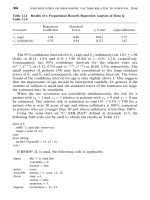
Table 12.1 Results of a Proportional Hazards Regression Analysis of Data in
Table 11.4
Regression Standard
Covariate Coefficient Error p Value exp(coefficient)
x

(age) 1.01 0.46 0013 2.75
x

(cellularity) 0.35 0.44 0.212 1.42
The 95% confidence intervals for b

(age) and b

(cellularity) are 1.01< 1.96
(0.46) or (0.11, 1.91) and 0.35 < 1.96 (0.44) or (90.51, 1.21), respectively.
Consequently, the 95% confidence intervals for the relative risks are
(e, e) or (1.12, 6.75) and (e\, e) or (0.60, 3.35), respectively. The
small number of patients (30) may have contributed to the large standard
errors of b

and b

and consequently, the wide confidence intervals. The lower
bound of the confidence interval for age is only slightly above 1. This suggests
that the importance of age should be interpreted carefully. In general, if the
number of subjects is small and the standard errors of the estimates are large,
the estimates may be unreliable.
When the two covariates are considered simultaneously, the risk for a
patient with x


: 1 and x

: 1 relative to patients with x

: 0 and x

: 0 can
be estimated. The relative risk is estimated as exp(1.01 ; 0.35) : 3.90 for a
patient who is over 50 years of age and whose cellularity is 100%, compared
to patients who are younger than 50 and whose cellularity is less than 100%.
Using the same data set ‘‘C:!AML.DAT’’ defined in Example 11.3, the
following SAS code can be used to obtain the results in Table 12.1.
data w1;
infile ‘c:!aml.dat’ missover;
input t cens x1 x2;
run;
proc phreg;
model t*cens(0) : x1 x2 / rl;
run;
If BMDP 2L is used, the following code is applicable.
/input file : ‘c:!aml.dat’ .
variables : 4.
format : free.
/print cova.
/variable names : t, cens, x1, x2.
/form time : t.
status : cens.
response : 1.
/regress covariates : x1, x2.
306        

If SPSS is used, the following code suffices.
data list file : ‘c:!aml.dat’ free
/ t cens x1 x2.
coxreg t with x1 x2
/status : cens event (1)
/print : all.
Example 12.2 In a study (Buzdar et al., 1978) to evaluate a combination
of 5-flourouracil, adramycin, cyclophosphamide, and BCG (FAC-BCG) as
adjuvant treatment in stage II and III breast cancer patients with positive
axillary nodes, 131 patients receiving FAC-BCG after surgery and radiation
therapy were compared with 151 patients receiving surgery and radiation
therapy only (control group).
Cox’s regression model was used to identify prognostic factors and to
evaluate the comparability of the two treatment groups. The model was fitted
to the data from 151 patients to determine the variables related to length of
remission. The possible prognostic variables considered were age (years),
menopausal status (1, premenopausal; 0, other), size of primary tumor (2, :3
cm; 4, 3—5 cm; 7, 95cm), state of disease (2, stage II; 3, stage III), location of
surgery (1, M. D. Anderson Hospital; 0, other), number of nodes involved (2,
:4; 7, 4—10; 12, 910), and race (1, Caucasian; 2, other). The covariates were
selected by the forward selection method outlined in Section 11.9. Three
variables — number of nodes involved, state of disease, and menopausal
status — were selected for use in the model, all related significantly (p : 0.1) to
disease-free time. The regression equation including these variables only is
log
h
G
(t)
h


(t)
: 0.111(number of nodes 9 6.16) ; 0.8122(stage 9 2.39)
; 0.872(menopausal 9 0.26)
Table 12.2 gives the details of the fit. Relative risk was taken as h
G
(t)/h

(t), the
ratio of the risk of death per unit of time for a patient with a given set of
prognostic variables to the risk for a patient whose prognostic variables were
average in value. The relative risk for each variable was calculated by
considering favorable or unfavorable values of that variable, assuming that
other variables were at their average value. Note that the risk of relapse per
unit time for a patient with 12 positive nodes is 3.04 (ratio or risk) times that
for a patient with only two positive nodes. The risk of relapse per unit time for
a stage III patient was 2.25 times that of a stage II patient.
The Cox’s regression model was also fitted to the combined group of
FAC-BCG and control patients, including type of treatment (0, control; 1,
FAC-BCG), menopausal status, size of primary tumor, and number of involved
nodes as potential prognostic variables. The regression equation with three
      307
Table 12.2 Patient Characteristics Related to Disease-Free Time in Cox’s Regression
Model Fit to Control Patients
Maximum Relative Risk?
Prognostic Regression Significance Log Ratio of
Variable Coefficient Level (p) Likelihood Favorable Unfavorable Risks
Number of
nodes 0.1110 :0.01 9257.407 0.63 1.91 3.04
Stage 0.8122 0.016 9254.533 0.73 1.64 2.25
Menopausal

status 0.8720 :0.1 9250.576 0.80 1.91 2.39
Source: Buzdar et al. (1978). Reprinted by permission of the editor.
? Favorable variables: number of nodes : 2, stage II, postmenopausal. Unfavorable variables:
number of nodes :12, stage III, premenopausal.
Table 12.3 Patient Characteristics Related to Survival, Treatment Included
Maximum Relative Risks?
Prognostic Regression Significance Log Ratio of
Variable Coefficient Level (p) Likelihood Favorable Unfavorable Risks
Treatment 91.8792 :0.01 9201.200 0.37 2.42 6.55
Menopausal 0.9644 0.01 9197.719 0.73 1.91 2.62
status
Size of 0.1611 0.05 9195.865 0.72 1.61 2.24
primary tumor
Source: Buzdar et al. (1978). Reprinted by permission of the editor.
? Favorable variables: treatment— FAC-BCG, postmenopausal, size of primary tumor 2 cm.
Unfavorable variables: no adjuvant treatment, premenopausal, size of primary tumor 7 cm.
significant (p : 0.05) variables obtained was as follows:
log
h
G
(t)
h

(t)
:91.8792(treatment9 0.47) ; 0.9644(menopausal status 9 0.33)
; 0.1611(size of primary tumor 9 4.04)
Table 12.3 gives the details of the fit. The most important variable in predicting
survival time was the type of treatment (FAC-BCG favorable); other signifi-
cantly important variables were menopausal status and size of primary tumor.
The risk of death per unit of time for a patient receiving no adjuvant treatment

(control group) was 6.55 times that for a patient receiving the treatment,
showing that FAC-BCG can prolong life considerably.
308        
Example 12.3 Suppose that demographic, personal, clinical, and labora-
tory data are collected from an interview and physical examination of 200
participants in a study of cardiovascular disease (CVD). These participants,
aged 50—79 years and free of CVD at the time of the baseline examination, are
then followed for 10 years. During the follow-up period, 96 of the 200
participants develop or die of CVD. We use this set of simulated data to
illustrate further the use of the proportional hazards model in identifying
important risk factors. Table 12.4 gives a subset of the simulated data of 68
participants.
The event time T of interest is CVD-free time, which is defined as the time
in years from baseline examination to the first time that a participant was
diagnosed as having CVD or confirmed as a CVD death. CVD includes
coronary heart disease (CHD) and stroke. The covariates of interest are age
(AGE), gender (SEX : 1 if male and :0 if female); smoking status
(SMOKE : 1 if current smoker, and 0 otherwise); body mass index
(BMI : weight in kilograms divided by height in meter squared); systolic
blood pressure (SBP); logarithm of ratio of urinary albumin and creatinine
(LACR); logarithm of triglycerides (LTG); hypertension status (HTN : 1if
SBP . 140 mmHg or DBP .90 mmHg or under treatments of hypertension,
and :0 otherwise); and diabetes status (DM: 1 if fasting glucose. 126
mg/dL or under the treatments of diabetes, and :0 otherwise). For the CVD
outcome of interest, we let DG denote the type of CVD. DG : 0 if the
participant is free of CVD at the end of the study or confirmed as a non-CVD
death (thus the CVD-free time is censored), :1 if the participant had a stroke,
:2 if the participant had a CHD, and :3 if the participant had other CVDs.
It is of interest to compare the risk of CVD among the three age groups: 50—59,
60—69, and 70—79. We create two dummy variables: AGEA : 1 if aged 50—69,

:0 otherwise; and AGEB: 1 if aged 60—69, and :0 otherwise. Thus for a 70
to 79-year-old, AGEA : 0 and AGEB : 0. We also create a variable to denote
the censoring status: CENS : 0 if t is censored, and : 1 if uncensored.
To illustrate the different methods to handle ties, we fit the Cox proportional
hazards model with the following six covariates: AGEA, AGEB, SEX,
SMOKE, BMI, and LACR. The approximated partial likelihood function
defined in (12.1.15)—(12.1.17) as well as the exact partial likelihood function
(Delong et al., 1994) are applied. As noted in Sections 11.3 and 11.4, the
exponential and Weibull regression models are also proportional hazard
models. Therefore, for comparisons we also fit an exponential and a Weibull
regression model with the same covariates to the data. The estimated re-
gression coefficients obtained from the proportional hazards model with
approximated discrete, Breslow, Efron, and exact partial likelihood functions
as well as those from the exponential and Weibull regression models are given
in Table 12.5. All of the estimates based on the Cox model and an approxi-
mated partial likelihood function are very closed to those based on the exact
partial likelihood. Those based on Efron’s approximation are almost identical
to those (different only at the fourth decimal place) based on the exact partial
      309
Table 12.4 A Subset of the Simulated Data for a Cardiovascular Disease Study in Example 12.3?
ID T CENS DG AGEA AGEB SEX SMOKE BMI SBP LACR LTG AGE HTN DM
1 7.4 0 0 0 0 0 0 31.78 141 4.23 3.94 77.8 1 0
2 7.9 0 0 0 0 0 0 25.02 124 4.31 4.66 76.9 0 1
3 6.4 0 0 0 0 0 1 26.05 111 4.38 4.27 76.3 0 0
4 7.1 0 0 0 0 0 1 26.92 140 1.11 4.51 72.2 1 0
5 6.0 0 0 0 0 0 1 34.30 146 1.19 4.82 76.0 1 0
6 6.5 0 0 0 0 0 1 31.76 142 1.20 4.88 74.5 1 0
7 8.3 0 0 0 0 1 0 25.01 154 3.53 4.10 70.7 1 1
8 7.9 0 0 0 0 1 0 28.21 136 3.73 4.12 75.2 1 0
9 7.6 0 0 0 1 0 0 28.13 127 2.92 4.24 64.9 0 0

10 8.4 0 0 0 1 0 0 25.68 118 2.47 4.41 60.2 0 0
11 7.4 0 0 0 1 0 0 34.34 118 2.37 4.46 64.4 0 1
12 7.7 0 0 0 1 0 0 28.92 127 3.58 4.55 68.8 1 1
13 6.9 0 0 0 1 0 1 24.68 100 2.11 4.33 64.4 0 0
14 7.2 0 0 0 1 0 1 21.93 121 3.39 4.64 60.8 0 1
15 6.3 0 0 0 1 0 1 29.47 98 1.96 4.69 64.4 0 0
16 7.4 0 0 0 1 0 1 28.65 150 2.59 4.95 61.6 1 0
17 4.5 0 0 0 1 1 0 32.28 128 2.99 4.73 65.3 0 0
18 7.0 0 0 0 1 1 0 29.21 117 2.17 4.91 65.7 0 1
19 2.8 0 0 0 1 1 0 28.82 136 4.04 4.92 65.4 0 1
20 7.2 0 0 0 1 1 0 30.58 121 2.84 4.94 64.5 0 1
21 7.4 0 0 1 0 0 0 27.83 95 1.85 4.44 52.0 0 0
22 5.2 0 0 1 0 0 0 26.61 128 2.87 4.51 50.7 0 0
23 7.7 0 0 1 0 0 0 30.32 96 2.41 4.60 52.5 0 1
24 7.8 0 0 1 0 0 0 30.41 130 1.45 4.73 55.9 0 0
25 7.6 0 0 1 0 0 1 29.98 140 1.88 4.51 53.4 1 0
26 7.9 0 0 1 0 0 1 26.00 118 2.34 4.53 51.0 0 0
27 7.3 0 0 1 0 0 1 29.05 110 1.44 4.67 50.6 0 0
310
28
8.2 0 0 1 0 0 1 27.21 131 2.50 4.68 57.7 0 0
29 3.8 0 0 1 0 1 0 36.97 141 4.60 4.25 58.7 1 0
30 6.9 0 0 1 0 1 0 29.44 115 2.89 4.26 53.6 0 1
31 6.1 0 0 1 0 1 0 33.85 154 3.48 4.48 51.2 1 0
32 7.2 0 0 1 0 1 0 32.13 122 2.92 4.48 55.2 0 0
33 8.4 0 0 1 0 1 1 27.52 135 2.39 4.42 53.7 0 0
34 5.0 0 0 1 0 1 1 30.64 114 1.39 4.45 54.9 1 0
35 6.5 0 0 1 0 1 1 29.94 120 2.96 4.49 50.7 0 0
36 6.4 0 0 1 0 1 1 29.89 115 1.68 4.52 51.3 0 0
37 2.6 1 1 0 0 0 0 30.88 189 5.38 4.72 73.9 1 1

38 2.7 1 1 0 0 0 1 25.05 200 3.37 4.86 77.2 1 1
39 2.7 1 1 0 0 1 0 26.80 130 2.31 5.10 73.5 0 0
40 3.3 1 1 0 0 1 1 21.67 111 3.53 4.18 71.1 0 0
41 2.9 1 1 0 1 0 0 36.83 114 2.64 4.52 68.2 0 0
42 0.2 1 1 0 1 0 1 21.49 125 4.61 4.69 67.3 0 0
43 2.1 1 1 0 1 1 0 31.05 131 1.38 4.48 69.1 0 0
44 6.8 1 1 0 1 1 1 26.78 134 4.36 4.90 61.0 1 0
45 5.7 1 1 1 0 0 0 35.78 132 9.93 5.11 52.5 0 1
46 1.1 1 1 1 0 0 1 28.44 134 3.54 4.32 55.7 0 0
47 6.6 1 1 1 0 1 0 24.38 124 4.16 4.00 51.8 0 1
48 1.3 1 1 1 0 1 1 34.13 126 5.87 3.95 53.1 0 1
49 4.6 1 2 0 0 0 0 43.23 128 5.08 5.25 72.2 0 1
50 6.3 1 2 0 0 0 1 38.67 126 5.16 4.50 76.8 1 1
51 2.0 1 2 0 0 1 0 34.49 130 2.69 3.95 76.7 1 1
52 4.2 1 2 0 0 1 1 20.78 127 4.40 4.54 73.1 0 0
53 3.6 1 2 0 1 0 0 28.40 118 5.43 4.66 69.3 1 1
54 3.2 1 2 0 1 0 1 28.73 154 1.94 5.24 68.9 1 1
55 4.5 1 2 0 1 1 0 44.25 97 2.01 4.40 68.6 0 1
56 4.5 1 2 0 1 1 1 32.46 141 0.74 4.39 63.5 1 0
57 6.1 1 2 1 0 0 0 39.72 118 2.39 3.93 52.6 0 1
(Continued overleaf )
311
Table 12.4 Continued
ID T CENS DG AGEA AGEB SEX SMOKE BMI SBP LACR LTG AGE HTN DM
58 3.0 1 2 1 0 0 1 27.90 117 7.45 5.61 56.0 0 1
59 2.1 1 2 1 0 1 0 27.77 119 7.03 4.71 54.3 0 1
60 1.3 1 2 1 0 1 1 31.03 151 3.94 4.43 59.2 1 1
61 4.9 1 3 0 0 0 0 25.22 129 6.69 3.90 75.4 1 0
62 2.5 1 3 0 0 0 1 45.29 130 2.46 4.40 75.7 0 1
63 3.8 1 3 0 0 1 0 25.03 188 6.25 5.63 71.7 1 1

64 5.0 1 3 0 1 1 0 46.76 96 3.93 4.12 65.6 1 0
65 1.5 1 3 0 1 1 1 28.53 126 3.09 4.65 68.6 0 1
66 4.1 1 3 1 0 0 0 23.63 144 8.24 4.82 59.4 1 1
67 0.5 1 3 1 0 1 0 31.39 134 6.96 4.11 54.2 1 0
68 2.7 1 3 1 0 1 1 30.29 115 4.70 4.98 59.1 1 1
? ID, participant id number; T, CVD event time (CVD-free time);CENS: 0 if censored, and :1 if uncensored; DG : 0ifnon-CVDat
the end of the study or non-CVD death, :1ifstroke,:2 if coronary heart disease (CHD),and:3 if the other CVDs; AGEA : 1if
aged 50—59 and :0otherwise;AGEB: 1ifaged60—69 and :0otherwise;SEX: 1ifmaleand:0 if female; SMOKE: 1ifcurrent
smoker and 0 otherwise; BMI, body mass index; SBP, systolic blood pressure; LACR, logarithm of the ratio of urinary albumin and
creatinine; LTG, logarithm of triglycerides; HTN: 1ifSBP.140 mmHg or DBP (diastolic blood pressure).90 mmHg and :0
otherwise; DM : 1 if fasting glucose.126 mg/dL and :0otherwise.
312
Table 12.5 Results from Fitting a Cox Proportional Hazards Model Based on Different
Methods for Ties on the CVD Data
Regression Coefficient
Variable Breslow Discrete Efron Exact Exponential Weibull
AGEA 91.3478 91.3662 91.3558 91.3560 91.2550 91.0436
AGEB 90.7709 90.7828 90.7753 90.7755 90.7107 90.5966
SEX 0.7134 0.7233 0.7187 0.7189 0.6862 0.5659
SMOKE 0.3762 0.3810 0.3776 0.3776 0.3440 0.2855
BMI 0.0253 0.0256 0.0255 0.0255 0.0233 0.0194
LACR 0.1735 0.1759 0.1739 0.1740 0.1658 0.1357
likelihood function. The estimated regression coefficients based on the two
parametric models, particularly the exponential regression model, are also
close to those based on the Cox hazards model. From the signs of the
coefficients, we see that men, current smokers, and persons with high BMI and
albumin—creatinine ratios have a higher hazard (risk) of CVD and shorter
CVD-free time. The coefficients of the two age variables are both negative,
indicating that persons in the younger age groups have a lower hazard (risk)
of CVD.

Suppose that ‘‘C:!EX12d2d1.DAT’’ contains eight successive columns, for T,
CENS, AGEA, AGEB, SEX, SMOKE, BMI, and LACR, and that the numbers
in each row are space-separated. The following code for the SAS PHREG and
LIFEREG procedures can be used to obtain the results in Table 12.5.
data w1;
infile ‘c:!ex12d2d1.dat’ missover;
input t cens agea ageb sex smoke bmi lacr;
run;
proc phreg;
model t*cens(0) : agea ageb sex smoke bmi lacr / ties : breslow;
run;
proc phreg;
model t*cens(0) : agea ageb sex smoke bmi lacr / ties : discrete;
run;
proc phreg;
model t*cens(0) : agea ageb sex smoke bmi lacr / ties : efron;
run;
proc phreg;
model t*cens(0) : agea ageb sex smoke bmi lacr / ties : exact;
run;
proc lifereg;
Model a: model t*cens(0) : agea ageb sex smoke bmi lacr / d : exponential;
Model b: model t*cens(0) : agea ageb sex smoke bmi lacr / d : weibull;
run;
      313
12.2 IDENTIFICATION OF SIGNIFICANT COVARIATES
As noted earlier, one principal interest is to identify significant prognostic
factors or covariates. This involves hypothesis testing and covariate selection
procedures, similar to those discussed in Chapter 11 for parametric methods.
The differences are that the Cox proportional hazard model has a partial

likelihood function in which the only parameters are the coefficients
associated with the covariates. However, statistical inference based on the
partial likelihood function has asymptotic properties similar to those based
on the usual likelihood. Therefore, the estimation procedure (discussed in
Section 12.1) is similar to those in Section 7.1, and the hypothesis-testing
procedures are similar to those in Sections 9.1 and 11.2. For example, the
Wald statistic in (9.1.4) can be used to test if any one of the covariates has no
effect on the hazard, that is, to test H

: b
G
: 0. By replacing the log-likelihood
function with the log partial likelihood function, the log-likelihood ratio
statistic, the Wald statistic, and the score statistic in (9.1.10), (9.1.11), and
(9.1.12) can be used to test the null hypothesis that all the coefficients are
equal to zero, that is, to test
H

: b

: 0, b

: 0, , b
N
: 0
or H

: b : 0 in (9.1.9). Similarly the forward, backward, and stepwise selection
procedures discussed in Section 11.9.1 are applicable to the Cox proportional
hazard model.

The following example, using the SAS PHREG procedure, illustrates these
procedures.
Example 12.4 We use the entire CVD data set in Example 12.3 to
demonstrate how to identify the most important risk factors among all the
covariates. Suppose that the effects of age, gender, and current smoking status
on CVD risk are of fundamental interest and we wish to include these variables
in the model. In epidemiology this is often referred to as adjusting for these
variables. Thus, AGEA, AGEB, SEX, and SMOKE are forced into the model
and we are to select the most important variables from the remaining
covariates (BMI, SBP, LACR, LTG, HTN, and DM), adjusting for age, gender,
and current smoking status.
The SAS procedure PHREG is used with Breslow’s approximation for ties
(default procedure) and three variable selection methods (forward, backward,
and stepwise). Two covariates, BMI and LACR, are selected at the 0.05
significance level by all three selection methods. The final model, in the form
of (12.1.5), including only the four covariates that we purposefully included and
the two most significant ones identified by the selection method, is
314        
Table 12.6 Asymptotic Partial Likelihood Inference on the CVD Data from the Final
Cox Proportional Hazards Model?
95% Confidence
Interval
Regression Standard Wald Relative
Variable Coefficient Error Statistic p Hazards Lower Upper
Final Model for the Cohort CV D Data
AGEA 91.3558 0.2712 24.9910 0.0001 0.258 0.151 0.439
AGEB 90.7753 0.2618 8.7709 0.0031 0.461 0.276 0.769
SEX 0.7187 0.2193 10.7457 0.0010 2.052 1.335 3.153
SMOKE 0.3776 0.2208 2.9235 0.0873 1.459 0.946 2.249
BMI 0.0255 0.0124 4.2113 0.0402 1.026 1.001 1.051

LACR 0.1739 0.0446 15.2112 0.0001 1.190 1.090 1.299
b

9 b

90.580 4.9443 0.0262 0.560
b

; b

1.096 11.5409 0.0007 2.993
b

9 b

0.341 1.3001 0.2542 1.407
Hypothesis Testing Results (H

: all b
G
: 0)
Log-partial-likelihood ratio statistic 42.1130 0.0001
Score statistic 43.1750 0.0001
Wald statistic 41.3830 0.0001
? The covariates, except AGEA, AGEB, SEX, and SMOKE, in the final model are selected among
BMI, SBP, LACR, LTG, HTN, and DM.
log
h(t
G
)

h

(t
G
)
: b

AGEA
G
; b

AGEB
G
; b

SEX
G
; b

SMOKE
G
; b

BMI
G
; b

LACR
G
:91.3558AGEA

G
9 07753AGEB
G
; 0.7187SEX
G
; 0.3776SMOKE
G
; 0.0255BMI
G
; 0.1739LACR
G
(12.2.1)
The regression coefficients, their standard errors, the Wald test statistics, p
values, and relative hazards (relative risks as they are termed by many
epidemiologists) are given in Table 12.6. The estimated regression coefficients
b
G
, i : 1, 2, . . . , 6, are solutions of (12.1.9) using the Newton—Raphson iterated
procedure (Section 7.1). The estimated variances of b
G
, i : 1, 2, , 6, are the
respective diagonal elements of the estimated covariance matrix defined in
(12.1.13). The square roots of these estimated variances are the standard errors
in the table. The Wald statistics are for testing the null hypothesis that the
covariate is not related to the risk of CVD or H

: b
G
: 0, i : 1, , 6, respect-
ively. For example, the Wald statistic equals 10.7457 for gender with a p value

    315
of 0.0010 and b : 0.7187. It indicates that after adjusting for all the variables
in the model (12.2.1), gender is a significant predictor for the development of
CVD, with men having a higher risk than women. The relative hazard (or risk)
is exp(b

), and for the covariate gender, it is exp(0.7187) : 2.052, which implies
that men aged 50—79 years have about twice the risk of developing CVD in 10
years. The 95% confidence interval for the relative risk is (1.335, 3.153), which
is calculated according to (7.1.8). For a continuous variable, exp(b
G
) represents
the increase in risk corresponding to a 1-unit increase in the variable. For
example, for BMI, exp (0.0255) : 1.026; that is, for every unit increase in BMI,
the risk for CVD increases 2.6%.
To compare hazards among different age groups, between genders, or
between smokers and nonsmokers, let h
%#
(t), h
%#
(t), h
%#!
(t), h
+*
(t),
h
$#+
(t), h
1+
(t), and h

,1+
(t) denote hazard functions for participants that are
50—59, 60—69, 70—79 years old, male, female, current smoker, and not current
smoker, respectively. The log hazard ratio of a person in the 50 to 59-year
age group to a person in the 70 to 79-year group assuming the two people are
of same gender and the same current smoking status, BMI and LACR, is
log[h
%#
(t)/h
%#!
(t)] : b

; similarly, log[h
%#
(t)/h
%#!
(t)] : b

and
log[h
%#
(t)/h
%#
(t)] : b

9 b

. Assuming that the two people are in the
same age group and have the same BMI and LACR, the log hazard ratio of
male to females is

log
h
+*
(t)
h
$#+
(t)
: b

Similarly, assuming that the two people are in the same age group, of the same
gender, and have the same BMI and LACR, the hazard ratio of a smoker to a
nonsmoker is
log
h
1+
(t)
h
,1+
(t)
: b

Thus, testing whether risk of CVD are the same among different age groups is
equivalent to testing H

: b

: 0, H

: b


: 0, and H

: b

9 b

: 0. Similarly, to
test if the risk of CVD is the same between males and females or between
smokers and nonsmokers is equivalent to tasting the null hypothesis H

: b

: 0
or H

: b

: 0, respectively.
To consider more than one covariate, we also can formulate the null
hypothesis by using (12.2.1). For example, if we wish to compare male
nonsmokers to female smokers, from (12.2.1),
log
h
+*\,1+
h
$#+\1+
: b

9 b


316        
assuming that they are in the same age group and have the same BMI and
LACR. Thus to test if these two groups of people have the same risk of CVD,
we test the null hypothesis H

: b

9 b

: 0. Similarly, to compare male
smokers to female nonsmokers, we can test the null hypothesis H

: b

; b

: 0.
These null hypotheses are in the form of linear combinations of the coefficients.
Using the notations in Section 11.2, the hypotheses H

: b

9 b

: 0 and
H

: b

; b


: 0 are the hypotheses in (11.2.13) with c : 0, L : (1 910000),
and L : (001100), respectively. The Wald statistics in Table 12.6 are
calculated according to (11.2.14). By assuming that the patients have the same
BMI and LACR, we can construct hypotheses to compare subgroups defined
by age groups, gender, and current smoking status.
The last part of Table 12.6 shows the results of testing the null hypothesis
that none of these covariates have any effect on the development of CVD. The
log partial likelihood ratio, Wald, and score statistics, X
*
, X
5
, and X
1
are
calculated according to (9.1.10), (9.1.11), and (9.1.12), respectively. Table 12.6
indicates that the hypotheses, H

: b

: 0, H

: b

: 0, H

: b

9 b


: 0,
H

: b

: 0, H

: b

: 0, H

: b

: 0, and H

: b

; b

: 0 are rejected at a signifi-
cance level of p : 0.05. However, the hypotheses H

: b

: 0 and
H

: b

9 b


: 0 are not rejected at a 0.05 level. The null hypothesis
H

: all b
G
: 0, i : 1, , 6, is rejected with p : 0.0001 by using any of these
tests.
Assuming that the other covariates are the same, based on the relative
hazards shown in the table, we conclude that (1) participants aged 50—59
and 60—69 have, respectively, about 25% and 50% lower CVD risk than
those aged 70—79 (H

: b

: 0 and H

: b

: 0 are rejected); (2) participants
aged 50—59 have 50% lower CVD risk than those aged 60—69 (H

: b

9 b

: 0
is rejected); (3) men’s CVD risk is twice as high as that of women (H

: b


: 0
is rejected); (4) BMI and LACR have a significant effect on CVD risk
(H

: b

: 0 and H

: b

: 0 are rejected) and the risk increases about 3% and
19%, respectively, for every 1-unit increase in BMI and LACR, respectively; (5)
male smokers have a CVD risk three times higher than that of female
nonsmokers (H

: b

; b

: 0 is rejected); (6) male nonsmokers have CVD risk
similar to that of female smokers (H

: b

9 b

: 0 is not rejected); (7) consider-
ing current smoking status alone, smokers had similar CVD risk as non-
smokers (H


: b

: 0 is not rejected). This example is solely for the purpose of
illustrating the use of the proportional hazards model and the interpretation
of its results. Other hypotheses of interest can be constructed in a similar
manner. The construction of null hypotheses for comparisons among sub-
groups defined by AGEGROUP*SEX*SMOKE are left to the reader as
exercises.
Suppose that ‘‘C:!EX12d4d1.DAT’’ is a text data file that contains
12 successive columns for T, CENS, AGEA, AGEB, SEX, SMOKE, BMI,
LACR, SBP, LTG, HTN, and DM. The following SAS code is used to obtained
the results in Table 12.6.
    317
data w1;
infile ‘c:!ex12d4d1.dat’ missover;
input t cens agea ageb sex smoke bmi lacr sbp ltg htn dm;
run;
proc phreg data : w1;
model t*cens(0) : agea ageb sex smoke bmi lacr sbp ltg htn dm /
include : 4 selection : f;
run;
proc phreg data : w1;
model t*cens(0) : agea ageb sex smoke bmi lacr sbp ltg htn dm /
include : 4 selection : b;
run;
proc phreg data : w1 outest : wcov covout;
model t*cens(0) : agea ageb sex smoke bmi lacr sbp ltg htn dm /
include : 4 selection : s;
run;

proc phreg data : w1;
model t*cens(0) : agea ageb sex smoke bmi lacr sbp ltg htn dm /
include : 4 selection : score best: 3;
run;
data wcov;
set wcov;
if
-
type
-
: ‘cov’;
keep agea ageb sex smoke bmi lacr sbp ltg htn dm;
run;
title ‘The estimated covariance of the estimated coefficients’;
proc print data : wcov;
run;
The following SPSS code can be used to select an optimal subset of
covariates among all covariates by the forward and backward selection
methods defined in Section 11.9.1 and to obtain the estimated coefficients and
the other results in Table 12.6.
data list file : ‘c:!ex12d4d1.dat’ free
/ t cens agea ageb sex smoke bmi lacr sbp ltg htn dm.
coxreg t with agea ageb sex smoke bmi lacr sbp ltg htn dm
/status : cens event (1)
/method : fstep bmi lacr sbp ltg htn dm
/criteria pin (0.05) pout (0.05)
/print : all.
coxreg t with agea ageb sex smoke bmi lacr sbp ltg htn dm
/status : cens event (1)
/method : bstep bmi lacr sbp ltg htn dm

/criteria pin (0.05) pout (0.05)
/print : all.
318        
If BMDP 2L is used, the following code is applicable when selecting an
optimal subset of covariates among all covariates by the stepwise selection
method defined in Section 11.9.1 and to obtain the results in Table 12.6.
/input file : ‘c:!ex12d4d1.dat’ .
variables : 12.
format : free.
/print cova.
/variable names : t,cens, agea, ageb, sex, smoke, bmi, lacr, sbp, ltg,
htn, dm.
/form time : t.
status : cens.
response : 1.
/regress covariates : agea, ageb, sex, smoke, bmi, lacr, sbp, ltg, htn,
dm.
Step : phh.
Example 12.5 If we do not force age, gender, and current smoking status
on the model and are not interested in the three age groups, we can fit the
proportional hazard model with age as a continuous variable and the other
covariates: SEX, SMOKE, BMI, SBP, LACR, LTG, HTN, and DM. Using
Breslow’s method for ties, the stepwise selection method, and the SAS pro-
cedure PHREG, the final model with significant (p : 0.05) covariates is
log
h(t)
h

(t)
: 0.697AGE ; 0.7528SEX ; 0.1111LACR; 0.3987LTG

(12.2.2)
The details are given in Table 12.7; all four covariates in the model have
positive coefficients, indicating that the risk of developing CVD increases with
age, gender, albumin/creatinine ratio, and triglyceride values. The relative
hazards represent the increase in risk of CVD per unit increase in the
covariates. For example, for every 1-unit increase in log(albumin/creatinine),
the risk of developing CVD increases 12% after adjusting for age, gender, and
log triglyceride. Men have more than twice the risk of CVD as women. The
global null hypothesis that all four coefficients equal zero (H

: all b
G
: 0) is
rejected by all three tests, as given in the lower part of Table 12.7.
12.3 ESTIMATION OF THE SURVIVORSHIP FUNCTION WITH
COVARIATES
When parametric regression models (Chapter 11) are used, we can estimate the
survivorship function simply by replacing the parameters and coefficients in the
survival function with their estimates. This is not the case when the Cox
       319
Table 12.7 Asymptotic Partial Likelihood Inference on the CVD Data from the Final
Cox Proportional Hazards Model Selected by the Stepwise Model Selection Method?
95% Confidence
Interval for
Relative Hazards
Regression Standard Chi-Square Relative
Variable Coefficient Error Statistic p Hazards Lower Upper
AGE 0.0697 0.0136 26.1393 0.0001 1.07 1.04 1.10
SEX 0.7528 0.2192 11.7893 0.0006 2.12 1.38 3.26
LACR 0.1111 0.0459 5.8602 0.0155 1.12 1.02 1.22

LTG 0.3987 0.1976 4.0722 0.0436 1.49 1.01 2.20
H

: All coefficients equal zero
Log-partial-likelihood ratio statistic 44.002 0.0001
Score statistic 44.278 0.0001
Wald statistic 42.527 0.0001
? The covariates in the final model are selected among AGE, SEX, SMOKE, BMI, LACR, LTG,
HTN, and DM using the stepwise selection method.
proportional hazards model is used since we do not know the exact form of
the baseline hazard function or the survival function. In this section we
introduce briefly two estimators of the survival function, one proposed by
Breslow (1974) and the other by Kalbfleisch and Prentice (1980). These
estimates are available in commercial software packages. Readers interested in
details are referred to the corresponding publications.
As indicated earlier, under the Cox model, the survivorship function with
covariates x
H
’s is
S(t, x) : [S

(t)]
exp(N
H
b
H
x
H
)
(12.3.1)

Once the regression coefficients, the b
H
’s, are estimated, we need only estimate
the underlying survivorship function, S

(t). From the estimated survivorship
function, we can easily estimate the probability of surviving longer than a given
time for a patient with a given set of covariates x

, , x
N
.
By assuming that the baseline hazard function is constant between each pair
of successive observed failure times, Breslow has proposed the following
estimator of the baseline cumulative hazard function:
H

(t) : 
t
G
-t
m
G

l + R(t
G
)
exp(x

J

b )
(12.3.2)
320        
Following (2.15), the baseline survival function can be estimated as
S

(t) : exp[9H

(t)] : 
t
G
-t

exp

m
G

l + R(t
G
)
exp(x

J
b )

(12.3.3)
and the survivorship function for a person with a set of covariates
x : (x


, , x
N
) is
S (t, x) : [S

(t)]
exp(N
H
b
H
x
H
)
: [S

(t)]
exp(bx)
(12.3.4)
Under mild assumptions, S (t, x) has an asymptotic normal distribution with
mean S(t, x). Since S(t, x) : exp[9H(t, x)], the variance estimator Var

(S (t, x))
of S (t, x) is
Var

(S (t, x)) < [S (t, x)] Var

(H (t, x))
We will not give H (t, x) here because of its complexity. The asymptotic
confidence bands for the survivorship function is

%S (t, x) 9 Z
?
(Var

(S (t, x)), S (t, x) ; Z
?
(Var

(S (t, x))& (12.3.5)
where Z
?
is the upper 100(1 9 /2) percentile point of the standard normal
distribution.
An alternative estimator has been suggested by Kalbfleisch and Prentice in
which the baseline survivorship function S

(t) is estimated to be a step function
and
S

(t) :
G\

H

H
t
G\
: t - t
G

, i : 1, , k ; 1 (12.3.6)
where 

Y 1 and 

, 

, ,
I
are the solution of the following k simultaneous
equations:

j + u*
G
exp(x

H
b )
1 9 
G
exp(x
H
b )
: 
l + R(t
G
)
exp(x

J

b ) i : 1, , k (12.3.7)
When there are no ties,

G
:

1 9
exp(x

G
b )

l + R(t
G
)
exp(x

J
b )

exp(9x
G
b )
i : 1, . . . , k (12.3.8)
and
S

(t) :
G\


H

1 9
exp(x

H
b )

l + R(t
H
)
exp(x

J
b )

exp(9x
H
b )
t
G\
- t :t
G
i : 1, , k ; 1
       321
Thus,
S (t, x) : [S

(t)]
exp(bx)

(12.3.9)
Under mild assumptions, the Kalbfleisch and Prentice estimator in (12.3.9) also
follows an asymptotic normal distribution with mean S(t, x) and a variance
that can be estimated. Thus confidence bands for the survivorship function can
also be constructed.
Using (12.3.4) with S

(t)in(12.3.3) or (12.3.6), the survivorship function can
be estimated with any given values of x

, , x
N
. If the observed average of
every covariate, x

, , x
N
is used, the estimated survivorship function can be
interpreted as the survivorship function of an ‘‘average’’ person.
Both the Breslow and Kalbfleisch—Prentice estimators are available in the
SAS procedure PHREG. The Breslow estimator is also available in BMDP
(program 2L) and SPSS (program COXREG). The following example illus-
trates the procedures.
Example 12.6 Again, we use the CVD data in the Example 12.3, the data
set ‘‘C:!EX12d2d1.DAT’’, and the SAS procedure PHREG. We use the average
of each of the covariates in (12.2.1), and therefore the estimated survivorship
function is for an average person. The Kalbfleisch—Prentice and Breslow
estimates of the survival function, defined in (12.3.9) and (12.3.4)(Efron
adjustment for ties is used), and the lower and upper 95% confidence bands,
calculated based on (12.3.5), are shown in Figures 12.1 and 12.2. These

estimated survival functions, using all the covariates in the model with average
values, are often referred to as the global covariate—adjusted survivorship
functions. The two figures are almost identical, which indicates that the two
methods produce very similar results for this set of data. From Figure 12.1 it
appears that the global covariates—adjusted survivorship function decreases
somewhat more rapidly after 3.5 years. This means that the process to develop
CVD accelerates after 3.5 years.
Using the data set ‘‘C:!EX12d2d1.DAT’’ defined in Example 12.3, the SAS
code used for this example is the following.
data w1;
infile ‘c:!ex12d2d1.dat’ missover;
input t cens agea ageb sex smoke bmi lacr;
run;
proc phreg data : w1 noprint;
model t*cens(0) : agea ageb sex smoke bmi lacr / ties : efron;
baseline out : base1 survival: survival l: lowb u : uppb / method : pl;
run;
title ’K-P estimate of the survival function and its lower and upper bands’;
proc print data : base1;
var t survival lowb uppb;
run;
322        
Figure 12.1 Kalbfleisch—Prentice estimate of survivorship function and its 95%
confidence bands at the averages of the covariates from the fitted Cox proportional
hazards model on the CVD data.
proc phreg data : w1 noprint;
model t*cens(0) : agea ageb sex smoke bmi lacr / ties : efron;
baseline out : base1 survival: survival l : lowb u : uppb / method : ch;
run;
title ’Breslow estimate of the survival function and its lower and upper bands’;

proc print data : base1;
var t survival lowb uppb;
run;
The following SPSS code can be used to obtain the Breslow estimate of the
survival function and its standard error at each uncensored observation. The
confidence bands can then be calculated according to (12.3.5).
data list file : ‘c:!ex12d2d1.dat’ free
/ t cens agea ageb sex smoke bmi lacr.
coxreg t with agea ageb sex smoke bmi lacr
/status : cens event (1)
/print : all.
       323
Figure 12.2 Breslow estimate of the survivorship function and its 95% confidence
bands at the averages of the covariates from the fitted Cox proportional hazards model
on the CVD data.
The corresponding BMDP 2L code is
/input file : ‘c:!ex12d2d1.dat’ .
variables : 8.
format : free.
/print cova.
Survival.
/variable names : t,cens, agea, ageb, sex, smoke, bmi, lacr.
/form time : t.
status : cens.
response : 1.
/regress covariates : agea, ageb, sex, smoke, bmi, lacr.
In addition to the global covariates—adjusted survivorship function defined
as S (t, x ), where x : (x

, x


, , x
N
), the survivorship function can be estimated
with any specific values of one or more of the covariates and interactions. We
can also estimate the probability of surviving longer than a given time for
individuals with a given set of values for covariates. The following is an
example.
324        
Figure 12.3 Breslow estimate of survivorship functions at the averages of BMI and
LACR from SEX*SMOKER subgroups in aged 70—79 participants from the fitted Cox
proportional hazards model on the CVD data.
Example 12.7 For the same model as in Example 12.6, we can estimate the
covariate-specific survivorship function for female nonsmokers, female
smokers, male smokers, and male nonsmokers. Let us use the 70—79 age group
and assume that BMI and LACR are at the average of the respective
SEX—SMOKE subgroup. Thus, the specific covariate vector (AGEA, AGEB,
SEX, SMOKE, BMI, LACR) for female nonsmokers is (0, 0, 0, 0, 30.69, 4.62),
where 30.69 and 4.62 are the average values of BMI and LACR for female
nonsmokers. Similarly, the specific covariate vectors for female smokers, male
nonsmokers, and male smokers are, respectively, (0, 0, 0, 1, 31.19, 2.67), (0, 0,
1, 0, 28.19, 3.43), and (0, 0, 1, 1, 25.76, 3.47). The estimated survival curves are
shown in Figure 12.3. Similarly, Figures 12.4 and 12.5 give the estimated
survival curves of the four groups in persons aged 60—69 years and 50—59
years, respectively. The groups show that in all these age groups, females have
a lower risk of developing CVD (longer CVD-free time) than males. Female
nonsmokers have a slightly lower risk than female smokers and the differences
increase as age decreases. However, among males, the differences in the risk of
CVD between smokers and nonsmokers are almost negligible in the youngest
group and much larger in the two older groups. Male smokers have the highest

risk of developing CVD (shortest CVD-free time) among the four groups.
       325
Figure 12.4 Breslow estimate of survivorship functions at the averages of BMI and
LACR from SEX*SMOKER subgroups in aged 60—69 participants from the fitted Cox
proportional hazards model on the CVD data.
12.4 ADEQUACY ASSESSMENT OF THE PROPORTIONAL
HAZARDS MODEL
The validity of statistical inferences that leads to the identification of important
risk or prognostic factors depends largely on the adequacy of the model
selected. The proportional hazards model is used widely in medical and
epidemiological studies. The adequacy of this model, including the assumption
of proportional hazards and the goodness of fit, needs to be assessed. In this
section we introduce several methods for this purpose. A major reason for
selecting these methods to present here is the availability of computer software
that can perform the calculations.
12.4.1 Checking the Proportional Hazards Assumption
The proportional hazards models defined in (12.1.1) and (12.1.3) assume that
the hazard ratio of two people is independent of time. This requires that
covariates not be time-dependent. If any of the covariates varies with time, the
proportional hazards assumption is violated. This fact can be used to test the
assumption by including a time—covariate interaction term in the model and
326        
Figure 12.5 Breslow estimate of survivorship functions at the averages of BMI and
LACR from SEX*SMOKER subgroups in aged 50—59 participants from the fitted Cox
proportional hazards model on the CVD data.
testing if the coefficient for interaction is significantly different from zero. For
example, we can add an interaction term x
G
t or x
G

log t in the model, that is,
log
h(t)
h

(t)
: b

x

; % ; b
G
x
G
; b
G
x
G
t ; b
G>
x
G>
; % ; b
N
x
N
or
log
h(t)
h


(t)
: b

x

; % ; b
G
x
G
; b
G
x
G
log t ; b
G>
x
G>
; % ; b
N
x
N
With the added interaction term, the partial likelihood function becomes more
complicated. Fortunately, computer software is available to carry out the
calculations. Testing procedures similar to those discussed earlier (e.g., the
Wald test), can be used to test the null hypothesis H

: b
G
: 0. If H


is rejected,
we conclude that Cox’s proportional hazard model is not appropriate for the
data. The interaction term with log t can be included in the model for each of
the covariates separately. If none of the corresponding p null hypotheses
H

: b
G
: 0 is rejected, we may conclude that the proportional hazards assump-
tion is appropriate.
       327
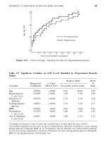
Table 12.8 Asymptotic Partial Likelihood Inference on the CVD Data from the Cox
Proportional Hazards Model with Time-Dependent Covariate
95% Confidence
Interval for
Relative Hazards
Regressor Regressor Standard Wald Relative
Variable Coefficient Error Statistic p Hazards Lower Upper
(a)
AGE 0.068 0.014 25.249 0.0001 1.07 1.04 1.1
SEX 0.759 0.218 12.056 0.0005 2.14 1.39 3.28
LACR 0.111 0.046 5.781 0.0162 1.12 1.02 1.22
LTG 0.915 0.435 4.420 0.0355 2.50 1.06 5.86
LTG* 90.390 0.298 1.710 0.1910 0.68 0.38 1.22
log(t;1)
(b)
AGE 0.071 0.014 26.635 0.0001 1.07 1.05 1.1
SEX 0.741 0.220 11.327 0.0008 2.10 1.36 3.23
LACR 90.087 0.120 0.519 0.4714 0.92 0.72 1.16

LTG 0.395 0.199 3.917 0.0478 1.48 1 2.19
LACR* 0.143 0.079 3.269 0.0706 1.15 0.99 1.35
log(t;1)
(c)
AGE 0.038 0.033 1.330 0.2488 1.04 0.97 1.11
SEX 0.764 0.220 12.020 0.0005 2.15 1.39 3.31
LACR 0.111 0.046 5.888 0.0152 1.12 1.02 1.22
LTG 0.417 0.197 4.469 0.0345 1.52 1.03 2.24
AGE*log(t
;1) 0.023 0.023 1.046 0.3064 1.02 0.98 1.07
Example 12.8 Consider the fitted proportional hazards model in (12.2.2) for
the CVD data. To check the proportional hazards assumption, we add a term
LTG;log(t ; 1) to the model. We use t ; 1 instead of t to avoid negative
values. Table 12.8(a) gives the results. The p value for the interaction term is
0.1910. Similarly, the results in Table 12.9(b) and (c) suggest that
LACR;log(t ; 1) and AGE;log(t ; 1) are not significant either. Since gender
is time-independent, we may conclude that the data satisfy the proportional
hazards assumption since every covariate in the model is time-independent.
Another method to check the proportional hazards assumption is to stratify
the data based on some values of a covariate, fit a stratified Cox proportional
hazards model (this is discussed in Chapter 13), and then construct the
survivorship function separately for the each stratum and plot
log(9log(S
H
(t; x
H
))) j : 1, 2, , m
328        
Figure 12.6 Log[9log(S(t))] plots for the age-stratified Cox proportional hazards
model on the CVD data.

against time t, where m is the number of strata defined by the covariate, x
H
is the
vector of the average values of the other covariates for the jth stratum, and S
H
(t; x
H
)
is the estimated survivorship function of the jth stratum evaluated at t and x
H
.If
the hazards are proportional, the m curves should be parallel. Nonparallel curves
indicate departure from the proportional hazards assumption. This is because if
hazard functions from any two people are proportional, it can be shown from
(12.1.1) that, for any j "k and 1 - j, k - m, there exists a constant d
HI
such that
S
H
(t; x
H
) : (S
I
(t; x
I
))B
HI (12.4.1)
Taking the logarithm twice, we have
log[9log(S
H

(t; x
H
))] : log d
HI
; log[9log(S
I
(t; x
I
))] (12.4.2)
Thus the curves of log[9log(S
H
(t; x
H
))] and log[9log(S
I
(t; x
I
))] versus t should
be parallel.
Example 12.9 Consider again the fitted model in (12.2.2); using the
stratified analysis (more details are given in Chapter 13), we plot
log[9log S
H
(t; x
H
)] against t for two age strata (50—64 and 65—79 years) and
two gender strata separately, where x
H
denotes the average values of the other
covariates for the jth stratum. These graphs are given in Figures 12.6 and 12.7,

       329
Figure 12.7 Log[9log(S(t))] plots for gender-stratified Cox proportional hazards
model on the CVD data.
respectively. The two curves in Figure 12.6 are roughly parallel. The two curves
in Figure 12.7 are also parallel over time. The results suggest that the
proportional hazards assumption holds.
In Chapter 11 we discussed several parametric models. Among these models,
the exponential and the Weibull are proportional hazards models, but the
others are not. Thus, if one of the other models provides a good fit to data, we
would know that the data do not meet the proportional hazards assumption.
This procedure can also be served as an alternative for checking the propor-
tional hazards assumption.
12.4.2 Assessing Goodness of Fit by Residuals
There are several other graphical methods available for assessing the goodness
of fit of a proportional hazards model. These graphical methods are based on
residuals and are often used as diagnostic tools. In multiple regression
methods, residuals are referred to as the difference between the observed and
the predicted values (based on the regression model) of the dependent variable.
However, when censored observations are present and only a partial likelihood
function is used in the proportional hazards model, the usual concept of
residuals is not applicable. In the following we introduce three different types
330        