Excel for Scientists and Engineers phần 5 pdf
Bạn đang xem bản rút gọn của tài liệu. Xem và tải ngay bản đầy đủ của tài liệu tại đây (3.25 MB, 48 trang )
170
EXCEL:
NUMERICAL
METHODS
Option Explicit
Function Bairstow(equation, reference)
'Obtains the coefficients of a regular polynomial (maximum order
=
6).
'Polynomial is a cell formula.
'Polynomial can contain cell references
or
names.
'Poynomial can be text.
'Reference can be a cell reference or a name.
Dim A() As Double, Root() As Double
Dim
J
As Integer, N As Integer
Dim pl As Integer, p2 As Integer, p3 As Integer
Dim expnumber As Integer, ParenFlag As Integer
Dim
R
As Integer, C As Integer
Dim FormulaText As String, Reffext As String, NameText As String
Dim char As String, term As String
ReDim A(6)
'
GET equation EITHER AS CELL FORMULA OR AS TEXT.
If
Application.lsText(equation)
Then
FormulaText
=
equation
'If
in quotes, remove them.
If
Asc(Left(FormulaText, 1))
=
34 Then
-
FormulaText
=
Mid(FormulaText, 2, Len(Formu1aText)
-
1)
Else
FormulaText
=
equation.Formula
End
If
If
Left(FormulaText, 1)
=
"="
Then FormulaText
=
Mid(FormulaText,
2,
1024)
FormulaText
=
Application.ConvertFormula(FormulaText,
xlAl
,
xlAl
,
-
FormulaText
= Application.Substitute(FormulaText,
"
'I,
"")
'remove all spaces
'GET THE NAME CORRESPONDING TO reference
NameText
=
""
On Error Resume Next 'Handles case where no name has been assigned
NameText
=
reference.Name.Name
On Error GoTo
0
NameText
=
Mid(NameText, InStr(1, NameText,
"!")
+
1)
'HANDLE CASE
WHERE
reference
IS
A RANGE
'by finding cell in same row or column as cell containing function.
If
reference.Rows.Count
>
1 Then
'
xlAbsolute)
R
=
equation.Row
Set reference
=
Intersect(reference, Range(R
&
":"
&
R))
C
=
equation.Column
Set reference
=
Intersect(reference, Range(C
&
":"
&
C))
Elself reference.Columns.Count
>
1 Then
This procedure contains code, not found in other procedures in this
book,
that
allows the macro to accept
a
polynomial equation as a reference to a cell that
contains a formula or as
a
reference to
a
cell that contains a formula as text.
The
procedure
also
handles an implicit reference.
CHAPTER
8
ROOTS
OF
EOUATIONS
171
End
If
Reffext
=
reference.Address
'PARSE THE FORMULA INTO TERMS
'pointers: pl, beginning; p2, end of string.
FormulaText
=
FormulaText
&
"
I'
'add extra character for parsing
ParenFlag
=
0
'Keep track of left and right parentheses
For J
=
1 To Len(Formu1aText)
char
=
Mid(FormulaText,
J,
1)
If
char
=
"("
Then ParenFlag
=
ParenFlag
+
1
If
char
=
")"
Then ParenFlag
=
ParenFlag
-
1
If
((char
=
"+"
Or char
=
"-")
And ParenFlag
=
0)
Or
J
=
Len(Formu1aText)
-
pl
=
1
Then
-term
=
Mid(FormulaText, pl
,
J
-
pl)
term
=
Application.Substitute(term,
NameText, Reffext)
p2
=
J: pl
=
p2
'GET THE EXPONENT AND COEFFICIENT FOR EACH TERM
'p3: location of reference
in
term.
If
InStr(1, term, Reffext &
'IA")
Then 'function returns zero if not found
'These are the x"2 and higher terms
p3
=
InStr(1, term, Reffext
&
""")
expnumber
=
Mid(term, p3
+
Len(Reffext)
+
1,
1)
term
=
Left(term, p3
-
1) 'term is now the coefficient part
Elself InStr(1, term, Reffext) Then
'This is the x term
p3
=
InStr(1, term, Reffext)
expnumber
=
1
term
=
Left(term, p3
-
1)
'term is now the coefficient part
Else
'This is the constant term
End
If
If
term
=
I"'
Then term
=
"=I" 'If missing, Evaluate will require a string.
If
term
=
"+"
Or term
=
"-"
Then term
=
term
&
"1"
If
Right(term, 1)
=
"*"
Then term
=
Left(term, Len(term)
-
1)
A(expnumber)
=
Evaluate(term)
End
If
Next
J
'RESIZE THE ARRAY
For J
=
6
To
0
Step -1
If
A(J)
<>
0
Then N
=
J: Exit For
Next
ReDim Preserve A(N)
ReDim Root(1 To N, 1)
'REDUCE POLYNOMIAL SO THAT FIRST COEFF
=
1
For J
=
0
To N: A(J)
=
A(J)
/
A(N): Next
'SCALE THE POLYNOMIAL, IF NECESSARY
'<code
to
be added later>
expnumber
=
0
172
EXCEL:
NUMERICAL
METHODS
Call
EvaluateByBairstowMethod(N, A, Root)
Bairstow
=
Root()
End Function
Sub
EvaluateByBairstowMethod(N,
A,
Root)
Code adapted from Shoup, "Numerical Methods for the Personal Computer".
Dim B() As Double, C()
As
Double
Dim M As Integer,
I
As
Integer,
J
As
Integer,
IT
As Integer
Dim P
As
Double, Q
As
Double, delP As Double, delQ As Double
Dim denom
As
Double, S1 As Double
Dim tolerance As Double
ReDirn B(N
+
2), C(N
+
2)
tolerance
=
0.000000000000001
M=N
While M
>
0
If
M
=
1 Then Root(M,
0)
=
-A(O):
Call
Sort(Root, N): Exit Sub
P
=
0:
Q
=
0:
delP
=
1
:
delQ
=
1
For
I
=
0
To N: B(I)
=
0:
C(I)
=
0:
Next
For
IT =
1
To 20
If
Abs(delP)
<
tolerance And Abs(delQ)
<
tolerance Then Exit For
For
J
=
0
To M
B(M
-
J)
=A(M
-
J)
+
P
*
B(M
-
J
+
1)
+
Q
*
B(M-
J
+
2)
C(M
-
J)
=
B(M
-
J)
+
P
*
C(M
-
J
+
1)
+
Q
*
C(M
-
J
+
2)
Next
J
denom
=
C(2)
A
2
-
C(l)
*
C(3)
delP
=
(-B(l)
*
C(2)
+
B(0)
*
C(3))
/
denom
delQ
=
(-C(2)
*
B(0)
+
C(l)
*
B(1))
I
denom
P
=
P
+
delP
Q
=
Q
+
delQ
Next
IT
S1
=PA2+4*Q
If
S1
i
0
Then
'Handle imaginary roots
Root(M,
0)
=
P
/
2:
Root(M, 1)
=
Sqr(-S1)
/
2
Root(M
-
1,
0)
=
P I2: Root(M
-
1, 1)
=
-Sqr(-S1)
/
2
'Handle real roots
Root(M,
0)
=
(P
+
Sqr(S1))
/
2
Root(M
-
1,
0)
=
(P
-
Sqr(S1))
/
2
Else
End
If
For
I
=
M To
0
Step -1: A(I)
=
B(I
+
2): Next
Wend
End Sub
'+++++++++i+++++++++++i+++++i+++i~++++++++i+++i++++i+++i+++
Sub Sort(Root, N)
'SORT ROOTS
IN
ASCENDING ORDER
Dim
I
As Integer,
J
As
Integer
M=M-2
CHAPTER
8
ROOTS
OF
EOUATIONS
173
Dim tempo
As
Double, templ
As
Double
For
I
=
1
To
N
For
J
=
I
To
N
If
Root(l,
0)
>
Root(J,
0)
Then
tempo
=
Root(l,
0):
temp1
=
Root(l, 1)
Root(l,
0)
=
Root(J,
0):
Root(l,
1)
=
Root(J, 1)
Root(J,
0)
=tempo: Root(J, 1)
=
templ
End
If
Next
J
Next
I
End
Sub
Figure 8-28.
VBA code for the Bairstow custom function.
(folder 'Chapter
08
Examples', workbook 'Bairstow', module 'BairstowFn')
The syntax of the Bairstow function is
Bairstow(
equation, reference)
Equation
is a reference to
a
cell that contains the formula of the function,
reference
is the cell reference of the argument to be varied (the
x
value of
F(x)).
To
return the roots of a
polynomial of order
N,
you must select a range of cells
2
columns by
N
rows,
enter the function and then press
CONTROL+SHIFT+ENTER.
The Bairstow function is an array function.
Figure
8-29
shows a chart of the polynomial
y=x3-0.0031x2+2.3
x
10-*x+5
x
lo-'
6.OE-09
T
5.OE-0
A
f::
//J
1.OE-09
f
-
-0.002
0.002
0.004
-1 .OE-09
-2.OE-09
I
Figure
8-29.
A
regular polynomial with one real root and
two
imaginary roots.
(folder 'Chapter
08
Examples', workbook 'Bairstow', sheet 'Example')
174
EXCEL: NUMERICAL METHODS
The function has one real root and a pair of imaginary roots. Figure
8-30
shows a portion of the spreadsheet in which the Bairstow custom function
is
used
to obtain the roots of the function.
Figure
8-30.
Calculation
of
all roots (real and imaginary)
of
a regular polynomial
by the Bairstow custom function.
(folder 'Chapter
08
Examples', workbook 'Bairstow', sheet 'Example
2')
The formula
=A2"3-0.0031
*A2"2+0.000000023*A2+0.000000005
was entered in cell B2 and the Bairstow custom function
{=Bairstow(B2,A2)}
in cells
A27:B29.
The real part of the root is in the left cell and the imaginary
part in the right cell. Note that, since the custom function handles only
polynomials with real coefficients, the complex roots (if any) occur in conjugate
pairs.
Finding Values Other than Zeroes
of
a Function
Many of the preceding methods can be modified
so
as to find the
x
of a
function for a
y
value other than zero. In this way you can find, for example, the
point of intersection of two curves (the
x
value where the
y
value of one function
equals they value of another function). Some examples follow.
Using
Goal
Seek
to Find the Point
of
Intersection
of
Two
Lines
It is a simple matter to use
Goal
Seek
to find the intersection of
two
lines,
as illustrated in Figure
8-3
1
CHAPTER
8
ROOTS
OF
EQUATIONS
175
120
100
80
60
40
20
0
-20
I
20
Figure 8-31.
Finding the intersection
of
two lines
in
a chart.
(folder 'Chapter
08
Examples',
workbook
'Intersecting Lines', sheet
'Two
Straight Lines')
In
the spreadsheet cells shown in Figure
8-32,
the formula
in
cell
824
is
=slope 1 *A24+ i n
t
1
and the formula in cell
C24
is
=slope2*A24+int2
Both formulas use
A24
as input. The formula
in
cell
D24
(the target cell)
is
=B24-C24
Now use
Goal Seek
to
vary
A24
to make the target cell,
D24,
equal to
zero. The result is shown in Figure
8-32.
Figure 8-32.
Using
Goal
Seek
to
find
the intersection
of
two lines.
(folder 'Chapter
08
Examples',
workbook
'Intersecting Lines', sheet
'Two
Straight Lines')
176
EXCEL: NUMERICAL METHODS
This approach is very simple, but it has one major drawback-you must run
Goal
Seek
.
each time you want to find the point of intersection.
A
much more
satisfactory approach is to use the Newton-Raphson technique to find the
intersection point, as illustrated in the following section.
The "drop line" in Figure 8-31 was added to the chart to emphasize the
intersection point. The line was added to the chart in the following way:
cell
A25
contains the formula
=A24
and cell
B25
contains the value
0.
The highlighted
cells
A24:B25
were copied and pasted in the chart to create a new series, as
follows:
Copy
A24:B25,
activate the chart, choose
Paste Special
from the
Edit
menu, check the boxes for Add Cells
As
New Series and
X
Values In First
Column, press
OK.
Figure 8-33 shows the portion of the worksheet where the
drop line is specified.
Figure
8-33.
Adding
a
"drop
line"
from
the intersection
of
two lines.
(folder 'Chapter
08
Examples',
workbook
'Intersecting Lines', sheet
'Two
Straight Lines')
Using the Newton-Raphson Method
to Find the Point of Intersection
of
Two
Curves
The Newton-Raphson method can be modified to find the
x
value that makes
a function have a specified value, instead
of
the zero value that was used in a
previous section. Equation
8-5
becomes
x2
=
(mxl
-y1
+y2)/m
(8-38)
You
can set up the calculation in the same way that was used for the Newton-
Raphson method with intentional circular reference. In the following example
we will find the intersection of
a
straight line and a curve (Figure 8-34).
CHAPTER
8
ROOTS
OF
EQUATIONS
177
300
250
200
150
100
50
0
5
10
15
20
-50
Figure
8-34.
Finding the intersection
of
two lines in a chart.
(folder 'Chapter
08
Examples', workbook 'Intersecting Lines', sheet 'Using Circular Reference')
A
portion
of
the data table that generated the
two
lines is shown in Figure
8-
35.
Figure
8-35.
Portion
of
the data table for Figure
8-32.
(folder 'Chapter
08
Examples', workbook 'Intersecting Lines', sheet 'Using Circular Reference')
The formula in cell
B5
is
=slope*AS+int
and
in
cell
C5
=aa*A5"2+ bb*A5+cc
Using the same method as in the preceding section,
y1
is
the function
for
which the slope
is
calculated, and
y2
is the value used as the "constant."
Of
course, both
yl
and
y2
change as the value of
x
changes.
178
EXCEL: NUMERICAL
METHODS
Figure
8-36.
Using
the Newton-Raphson method
to
find the intersection
of
two
lines.
(folder 'Chapter
08
Examples',
workbook
'Intersecting Lines', sheet 'Using Circular Reference')
Figure
8-36
shows the cells where the Newton-Raphson calculation
is
performed, using an intentional circular reference (refer to the section "The
Newton-Raphson Method Using Circular Reference and Iteration" earlier in this
chapter if the method of calculation is not apparent). The formula in cell
G38
is
=(C38+F38*A38-B38)/F38
The advantage of using the Newton-Raphson method with circular
references, compared to using
Goal
Seek
,
is
that calculation
of
the
x,
y
coordinates of the intersection occurs automatically, "in the background." If you
change one or more of the parameters (for example, if you change the slope
of
the straight line), the new intersection point and new drop line will be calculated
and displayed on the chart.
Using the Newton-Raphson Method
to Find Multiple Intersections
of
a
Straight Line and a Curve
The preceding technique can be easily extended to find multiple intersections
of
two
curves. The following figure illustrates how to find the
two
intersections
of a horizontal straight line with
a
parabola, but many other types of curve can be
handled.
CHAPTER
8
ROOTS
OF
EQUATIONS
179
600
-
500
-
400
-
300
-
200
'
100
I
-30
-20
-10
0
10
20
30
Figure
8-37.
Two intersections of a straight line and a curve, calculated by using the
Newton-Raphson method
with
intentional circular references.
(folder 'Chapter
08
Examples',
workbook
'Intersecting Lines', sheet 'Using Circular Reference
(2)')
It is merely necessary to use
two
identical Newton-Raphson formulas and
provide
two
different start values that will result in convergence to the
two
different "roots."
Figure
8-38
illustrates the set-up of the table. Cells
C66
and
C67
contain the formula
=$1$5
(pointing to the cell that contains a constant). Guided by Figure
8-37,
initial
x
values of
10
and
-10
were chosen. Figure
8-38
shows the cell values before the
intentional circular references have been created.
Figure
8-38.
Calculating two intersections of a line and
a
curve
by
the Newton-Raphson method (before creating intentional circular references).
(folder 'Chapter
08
Examples',
workbook
'Intersecting Lines', sheet 'Using Circular Reference
(2)')
Once the formulas have been entered, replace the initial
x
values in cells
A66
and
A67
by the formulas
=G66
and
=G67,
respectively, to create the
two
circular
references. The "Cannot resolve circular references" message will be displayed
180
EXCEL: NUMERICAL METHODS
and the
two
cells will display zero values. Now choose
Options
from the
Tools
menu and choose the Calculation tab. Check the Iteration box and press
OK.
Figure
8-39
shows the final values in the table, after circular reference
iteration is complete.
Figure 8-39.
Calculating two intersections of a line and a curve
by
the Newton-Raphson method (after creating intentional circular references).
(folder 'Chapter
08
Examples',
workbook
'Intersecting Lines', sheet 'Using Circular Reference
(2)')
A
Goal
Seek Custom Function
The Newton-Raphson custom function described in
a
previous section was
modified to create
a
custom function that performs goal seeking. This custom
function can be used in the same way as Excel's built-in
Goal
Seek
tool
-
to
find the value of
x
(the changing cell) that makes the function
y
(the target cell)
have
a
specified value. The
VBA
code is shown in Figure
8-40.
Option Explicit
Function GoalSeek(target-cell, changing-cell, objective-value, Optional
-
initial-value) As Double
'Finds value
of
X to make
Y
have a desired value
'This is a modified version of NewtRaph
Dim tolerance
As
Double, incr As Double
Dim XRef As String, Formulastring As String
Dim
I
As
Integer
Dim XI As Double,
Y1
As Double, X2 As Double,
Y2
As
Double
Dim
m
As
Double
If
IsMissing(initia1-value)
Then initial-value
=
changing-cell
If
initial-value
=
I"'
Then initial-value
=
changing-cell
tolerance
=
0.0000000001
incr
=
0.00000001
XRef
=
changing-celI.Address
Formulastring
=
target-cell.Formula
Formulastring
=
Application.ConvertFormula(FormulaString,
xlAl
,
xlAl
,
-
xl Absolute)
CHAPTER
8
ROOTS
OF
EQUATIONS
181
XI
=
initial-value
For
I
=
1
To
100
Y1
=
Evaluate(Application.Substitute(FormulaString,
XRef,
XI))
If
XI
=
0
Then
XI
=
incr
X2 =XI
+
XI
*
incr
Y2
=
Evaluate(Application.Substitute(FormulaString,
XRef,
X2))
m
=
(Y2
-
Y1)
I
(X2 -XI)
X2
=
(m
*
XI
-
Y1
+
objective-value)
I
m
'Exit here if
a
root
is found
If
Abs((X2
-
XI)
I
X2)
c
tolerance
Then
GoalSeek
=
X2:
Exit Function
XI =x2
Next
I
'Exit here with error value if no
root
found
GoalSeek
=
CVErr(x1ErrNA): Exit Function
End Function
End Sub
Figure
8-40.
VBA code for
the
GoalSeek custom function.
(folder 'Chapter
08
Examples', workbook 'GoalSeek Fn', module 'Module
1')
This custom function can be used in the same way as Excel's built-in
Goal
Seek
.
tool to find the value of
x
(the changing cell) that makes the function
y
(the target cell) have a specified value.
The syntax of the function is
GoaISeek(target-cel/, changing-cell, objective-value,
initial_value)
The argument
targetcell
is
a reference to a cell containing a formula
F(x).
The argument
changing-cell
is
a cell reference corresponding to
x,
the
independent variable. (The formula in
fargef-cell
must depend on
changing-cell.)
These
two
arguments correspond exactly to the
Goal
Seek
tool's
inputs Set Cell and By Changing Cell. The argument
objective-value
(Goal
Seek's
To Value input) is the value you want
fargef-cell
to attain. The optional
argument
inifial_value
is used, in cases where more that one value of
x
can result
in the function
F(x)
having the desired value, to control the value of
x
that is
returned.
Note that when using the
Goal
Seek
tool, To Value can only be a fixed
value, not a cell reference, whereas when using the
GoalSeek
custom function,
the argument can be a cell reference. Thus, when
objecfive-value
is changed, the
GoalSeek
return value updates automatically.
As
an illustration, we will use the
GoalSeek
custom function to find the
value
of
x
that makes the function
y
=
x2
+
6x
-10 have a specified value, namely
y
=
210.
In the spreadsheet shown in Figure 8-41 the table in
$A$5:$B20
provides the
x,
y
values of the function that are plotted in Figure 8-42. The
adjustable parameters of the function are in
$E$5:$E$7.
The adjustable value of
the intersection point
H
is in cell
E10.
Cell
D14
contains the formula
182
EXCEL: NUMERICAL METHODS
=goalseek(B5,A5,ElO)
Note that the
GoalSeek
function does not modify the value of the changing
cell (in this example cell
A5)
nor does it result in a change in the
cell
containing
the function (in this example cell
85).
These values are merely copied and used
as inputs for the
VBA
code. The final value
of
the changing cell is returned by
the
GoalSeek
function (in this example in cell
D14).
As
a
check, the target cell
formula was entered in cell
El4
so
as to calculate
F(x)
using the value
of
x
returned by
Goalseek.
Some functions have more than one value of
x
that can satisfy the
relationship
F(x)
=
objective-value;
in these cases the user must use the optional
argument
initial_va/ue
to control the value of
x
that is returned.
Figure
8-41.
Using the GoalSeek custom function to find the value
ofx
that makes the function
y
=
x2
+
6x
-
10
have a specified value (here,
y
=
2
10).
(folder 'Chapter
08
Examples',
workbook
'Goalseek
Fn',
sheet 'Intersection
of
line
with
h
(2)')
If you change the values of
aa,
bb,
cc,
or
H,
the function value will update to
find the new intersection value. In contrast, if you use the
Goal
Seek
.
tool, you
CHAPTER
8
ROOTS
OF
EQUATIONS
183
must repeat the action of goal-seeking each time you change any
of
the
parameters.
A
limitation of the
GoalSeek
custom function is that
fargetcell
must contain
the complete expression dependent on
changing-cell.
Only
the instances
of
changing-cell
that appear in the formula in
targef-cell
will be used in the
Newton-Raphson calculation.
300
250
200
>
150
100
50
0
-50
1
5
10
X
15
Figure
8-42.
The value
of
x
that makes the
function
y
=
x2
+
6x
-
10
have the value
210.
(folder 'Chapter
08
Examples', workbook 'Goalseek Fn'. sheet 'Intersection
of
line with
h
(2)')
The CD contains an example of the use of the
GoalSeek
function to find
approximately
180
intersection points of lines with a curve in
a
chart (see folder
'Chapter
08
Examples', workbook 'Diatomic Molecule', sheet 'Vibrational Energy
Levels').
The resulting chart
is
shown in Figure
8-43.
The chart contains
two
data series. The first data series shows the continuous function of energy as a
function of distance
r.
The second data series shows the approximately
90
horizontal vibrational energy levels.
184
EXCEL: NUMERICAL
METHODS
200
180
160
140
120
7
Y
s
Q
100
Q)
c
w
80
60
40
20
0
t
2
4 6
lnternuclear distance,
A
Figure
8-43.
Using
the
GoalSeek
custom function
to
find
multiple intersections
of
lines in a chart.
(folder 'Chapter
08
Examples',
workbook
'Diatomic Molecule', sheet 'Sheetl')
8
CHAPTER
8
ROOTS
OF
EQUATIONS
185
Problems
Answers to the following problems are found in the folder "Ch.
08
(Roots of
Equations)"
in
the "Problems
&
Solutions" folder on the CD.
1. A circuit consisting of
a
source,
a
resistor and a load, has a current
i
that
oscillates as a function of time
t
according to the following:
7T
7T
i
=
2.5 sin(-)e-2.5'
+
2.5 sin(2.5t
-
-)
4
4
Find the first time after t
=
0
when the current reaches zero.)
2. In pipe flow problems the relationship
is encountered. Solve for
D,
if
a
=
700,
b
=
-2.9,
c
=
-300.
aD3
+
bD
+
c
=
0
3.
When the sparingly soluble salt BaC03 is dissolved in water, the following
simultaneous equilibria apply:
BaC03
e
Ba2++ C03'-
Ksp
=
[Ba2'][C032-]
=
5.1
x
lo-'
C0:-
+
H20
+
HCO<
+
OH-
Kb
=
[OH-][ HCO<]/[ C032-]
=
2.1
x
lo4
Employing mass- and charge-balance equations, the following relationship
can be obtained for a saturated solution of BaC03 in water:
[Ba2+I2
-
JKbKsp
[Ba2+]1'2
-
Ksp
=
0
Find the concentration of free Ba2' in the saturated solution.
4.
A solution of
0.10
M
nitric acid
(HNO3)
is
saturated with silver acetate
(AgAc), a sparingly soluble salt. The system of mass- and charge-balance
equations describing the system is
NO^-]
=
0.1
o
(mass balance)
[Ag']
=
S
(mass balance)
[Ac-]
+
[HAc]
=
S
(mass balance)
[Ag']
+
[W]
=
[Ac-]
+
[NOS-]
(charge balance)
[Ag'][Ac-]
=
4.0
x
KSp
[H'][Ac-]/[HAc]
=1.8
x
KO
186
EXCEL: NUMERICAL METHODS
5.
6.
7.
8.
where
S
is the mol/L of silver acetate that dissolve. Using the preceding
relationships, the following expression is obtained for the solubility
S
of
silver acetate:
KO[
-
1)
+
S
=
7
K,
+
0.10
Find the solubility
S.
Find the two sets of coordinates of the intersection of the straight line
y
=
mx
+
b,
where
m
=
5
and
b
=
50,
with the parabola
y
=
ax2
+
bx
+
c,
where
a
=
1.1,
b
=
-2.3
and
c
=
-30.5.
Make a chart of the two series to show the
intersections.
Find the
two
sets
of coordinates of the intersection of the straight line with
y
=
h
and the circle of radius
r
(the equation of a circle is
x2
+
y2
=
r;
thus
y
=
43
).
For example, use r
=
1
and
h
=
some value between
0
and
1.
The intersections will be at
x,
y
=
h
and
-x,
y
=
h.
Make
a
chart to show the
circle (values of
x
from
-1
to
1
and calculated values of
y,
also same values
of
x
and
-y).
Having solved problem
#8,
and having created the chart, use the values of the
intersections to create
a
chart series that shows the circumscribed rectangle
(four sets of coordinates:
x,
y
=
h;
-x,
y
=
h;
x,
y
=
-h;
-x,
y
=
-h).
Use any
suitable method to find the coordinates of the circumscribed square.
For the chemical reaction
2A=B+2C
the equilibrium constant expression
is
For this reaction, the value of the equilibrium constant
K
at a certain
temperature is
0.288
mol
L-I.
A
reaction mixture is prepared in which the initial concentrations are
[A]
=
1,
[B]
=
0,
[C]
=
0
mol
L-I.
From mass balance and stoichiometry, the
concentrations at equilibrium are
[A]
=
1
-
2x,
[B]
=
x,
[C]
=
2x
mol L-',
from which the expression for
K
is
.
Find the value of
x
that
4x3
1
-
4~
-
4x2
CHAPTER
8
ROOTS OF
EOUATIONS
187
makes the expression have
a
value of 0.288, and calculate the concentrations
of A,
B
and C at equilibrium.
9. For the gas-phase chemical reaction
the equilibrium constant expression for reaction is
A
+
B
+
C
+2D
K=
[c1[D12
=
15.9 atm at 400°C.
[A1
[Bl
A reaction mixture is prepared in which the initial concentrations are [A]
=
1
atm,
[B]
=
2 atm, [C]
=
0,
[Dl
=
0.
From mass balance and stoichiometry,
the concentrations at equilibrium are [A]
=
1
-
x,
[B]
=
2
-
x,
[C]
=
x,
[D]
=
4x
3
X’
-3xi-2
2x, from which the expression for
K
is
.
Find the value of x that
makes the expression have a value of 15.9, and calculate the partial pressures
of A,
B,
C and D at equilibrium.
10.
The Reynolds number
is
a dimensionless quantity used in calculations of
fluid flow in pipes. The Reynolds number
is
defined as
where
Di
is
the inside diameter of the pipe,
V
is the average velocity of the
fluid in the pipe,
p
is
the fluid density and
p
is the absolute viscosity of the
fluid. For flow in pipes, a Reynolds number of less than 2000 indicates that
the flow
is
laminar, while a value of greater than
10,000
indicates that the
flow is turbulent. For a pipe diameter of
5
cm, and fluid of density
1
g/cm3
and viscosity of
1
centipoise, find the minimum velocity that results in
turbulent flow.
1
1.
Find the value of the
(1,l)
element of the following matrix that gives a
determinant value of zero.
0.75 0.5
0.25
[
0.5
1
0.51
0.25
0.5
0.75
Which elements in the matrix cannot be changed in order to give a
determinant of zero?
12.
Use the Bairstow custom function to find all of the roots of the polynomial
188 EXCEL: NUMERICAL METHODS
X5-
1oX4+30X3-20X2-31X+30
13.
Use the Bairstow custom function to find
all
of
the roots
of
the polynomial
16200000~~
-
64800000~~
+
97 199996~~
-
64800000~
+
16200000
Chapter
9
Systems
of
Simultaneous Equations
Sometimes a scientific
or
engineering problem can be represented by a set of
n
linear equations in
n
unknowns, for example
x+2y=
15
3x+
8y=
57
or,
in the general case
allxl
+
a12x2
+
a13x3
+
“’
+
al&,x,,
=
c1
~~21x1
+
~22x2
+
~23x3
+
+
~2,&,,
=
~2
a17lX1
+
am
+
a,43
+
*
*
+
a,,,&,,
=
c,
where
xl,
x2,
x3,
,
x,
are the experimental unknowns,
c
is
the experimentally
measured quantity, and the
aii
are known coefficients.
The equations must be
linearly independent; in other words, no equation is simply a multiple of another
equation,
or
the sum of other equations.
A
familiar example
is
the spectrophotometric determination of the
concentrations of a mixture of
n
components by absorbance measurements at
n
different wavelengths. The coefficients
ay
are the
E,
the molar absorptivities of
the components at different wavelengths (for simplicity, the cell path length,
usually
1.00
cm, has been omitted from these equations).
For
example, for a
mixture
of
three species
P,
Q and R, where absorbance measurements are made
at
hl,h2
and
h3,
the equations are
E
1,
[PI
+
E?,
[QI
+
E:,
[RI
=An,
E:~
[PI
+
E:,
[QI
+
&f2
[RI
=A,,
&I,
[PI
+
&??
[QI
+
~n”,
[RI
=A,,
This chapter describes direct methods (involving the use of matrices) and
indirect (iterative) methods for the solution of such systems. The chapter begins
189
190
EXCEL:
NUMERICAL
METHODS
D=
by describing methods for the solution of systems of linear equations, and
concludes by describing
a
method for handling nonlinear systems of equations.
2 1
-1
1 -1 1
121
Cramer's Rule
According to Cramer's rule, a system of simultaneous linear equations has a
unique solution if the determinant
D
of
the coefficients is nonzero. To obtain the
solution, each unknown is expressed
as a
quotient of
two
determinants: the
denominator
is
D
and the numerator is obtained from
D
by replacing the column
in the determinant corresponding to the desired unknown with the column of
constants.
Thus, for example, for the set of equations
2x
+
y
-
z
=
0
x-y+z=6
x
+
2y
+
z
=
3
The coefficients and constants lend themselves readily to spreadsheet
solution, as illustrated in Figure
9-1.
Using the formula
=MDETERM(AZ:C4),
the
value
of
the determinant is found to be
-9,
indicating that the system is soluble.
Figure
9-1.
Spreadsheet data
for
three equations in three unknowns.
(folder 'Chapter
09
Simultaneous Equations', workbook
'Simult
Eqns
1',
sheet 'Cramer's Rule')
Figure
9-2.
The determinant
for
obtaining
x.
(folder 'Chapter
09
Simultaneous Equations', workbook 'Simult Eqns
I',
sheet 'Cramer's Rule')
CHAPTER
9
SYSTEMS
OF
SIMULTANEOUS EOUATIONS
191
The
x
values that comprise the solution
of
the set of equations can be
calculated in the following manner:
xk
is given by a quotient in which the
denominator is
D
and the numerator is obtained from
D
by replacing the
gh
column of coefficients by the constants
c,,
cz.
The unknowns are obtained
readily by copying the coefficients and constants to appropriate columns in
another location in the sheet. For example, to obtain
x,
the determinant is shown
in Figure
9-2,
and
x
=
2
is obtained from the formula
=MDETERM(A8:CI O)/MDETERM(A2:C4)
y
=
-1
and
z
=
3
are obtained from appropriate forms of the same formula.
only a few equations.
Cramer's method is very inefficient and should be used only for systems of
Solving Simultaneous Equations
by
Matrix Inversion
Simultaneous equations can be represented in matrix notation by
Ax=C
(9-
1
)
X
=
A-'C
(9-2)
where
A
is
the matrix of coefficients,
B
the matrix of unknowns, and
C
the
matrix of constants. Multiplying both sides of equation
9-1
by
A-'
yields
In other words, the solution matrix is obtained by multiplying the matrix of
constants by the inverse matrix of the coefficients.
To
return the solution values
shown in Figure
9-3,
the array formula
{=MMULT(MINVERSE(A2:C4),D2:D4)}
was entered in cells
E2:E4.
Figure
9-3.
Solving a set
of
simultaneous equations
by
means
of
matrix methods.
(folder 'Chapter
09
Simultaneous Equations',
workbook
'Simult Eqns
1',
sheet 'Matrix Inversion')
Solving Simultaneous Equations
by
Gaussian Elimination
A
system of linear equations such as
x+2y=
15
3x+Sy=57
192
EXCEL: NUMERICAL METHODS
can be solved by successive substitution and elimination of variables. For
example, you can multiply the first equation by
3,
so
that the coefficient of
x
is
the same as in the second equation, and then subtract it from the second equation,
thus
3x+Sy=57
-3x
+
6~45
2y= 12
to produce a single equation in one unknown from which
y
=
6.
Using the value
of
y,
you can now calculate
x.
To extend this procedure to
a
system of
n
equations in
n
unknowns requires
that one work in
a
systematic fashion. The solution process is equivalent to
converting the
n
x
n
matrix above into a triangular matrix, such
as
the upper
triangular matrix
allxi
+
~12x2
+
a193
+
+
=
bl
a22x2
+
a23x3
+
.
.
+
a2$"
=
b2
a33x3
+
+
a3dn
=
b3
andn
=
bn
which corresponds to a system of equations in which one of the equations
contains only one unknown, and successive equations contain only one additional
unknown.
A
similar solution process can be carried out using a lower triangular
matrix.
There are several methods for the solution of systems of equations that
involve a triangular matrix. The Gaussian elimination process reduces
a
system
of linear equations to an upper triangular matrix. In the example
at
the beginning
of this chapter, we used the first equation to eliminate
x1
from the other equation.
To eliminate
x1
in
a
system
of
n
equations:
allxl
+
a12x2
f
013x3
+
+
al$n
=
bl
~21x1
+
~22x2
+
a293
+
.*.
+
a2dn
=
b2
a31x1
+
~32x2
+
~33x3
+
+
a3dn
=
b3
etc.
we multiply equation
1
by the factors azl/all,
a31/a11,
,
a,l/all and subtract from
equations
2,
3,
,
n.
This eliminates
x1
from equations 2 n. Equation
1
is
termed the pivot equation, and the coefficient of
x1
the
pivot.
We then use equation
2
as
the pivot equation, the coefficient
of
x2
as
the
pivot, and eliminate
x2
from equations
3,
. .
.
,
n.
-
1 0.2 0.2 0.2 137
2
-1
-1
1
165
3
-1
2
-2 256
5 -4
3
-2 361
-
:
CHAPTER
9
SYSTEMS
OF
SIMULTANEOUS EOUATIONS
193
If the pivot equation is normalized by dividing it by the coefficient of
xJ,
the
It
will be instructive to show the progress of the calculations with a simple
coefficient of
x,
is
1
and the calculations are simplified somewhat.
example, such as the following:
The Gaussian elimination method operates on an
n
x
n
matrix of coefficients,
augmented by the vector of constants. In our example this matrix will be a
4
x
5
matrix, as shown:
First, row
1
is normalized:
The
x1
terms are eliminated from column
1
of rows 2,3 and
4
by subtracting:
Row 2 is normalized:
The
x2
terms are eliminated from column 2 of rows 3 and
4:
194
EXCEL:
NUMERICAL
METHODS
1 0.2 0.2 0.2
0
1 1 -0.4286 77.::;]
0 0
3
-3.2857 -30.429
I
0 0
7 -5.1429 65.286
Row
3
is
normalized and the
x3
terms are eliminated from column
3
of row
4:
1 0.2 0.2 0.2 137
0
1
1 -0.4286 77.857
0
0
1
-1.0952 -10.143
0 0 0
2.5238 136.29
1 0.2
0.2 0.2
o
1
1 -0.4286 77,KI
I
1
000
1
54
Row
4
is normalized:
0 0
1 -1.0952 -10.143
As
you can see, the coefficients matrix
is
now an upper triangular matrix,
with the diagonal elements equal to one. The results are obtained by successive
substitution, beginning with the last row. The last row corresponds to
x4
=
154,
the third row corresponds
to
x3
-
0.272727~4
=
107,
from which
x3
=
149,
and
so
on. The results,
XI,
x2, x3
and
x4
are
106, 52, 49, 54,
respectively.
You can see
the steps in Gaussian elimination calculation by using the demo program
provided on the
CD
(folder 'Chapter
09
Simultaneous Equations', workbook
'Simult Lin Eqns', sheet 'Gaussian Elimination Demo').
The Gaussian elimination method can also be performed by using the
VBA
custom function
GaussElim.
The
VBA
code
is
shown in Figure
9-4.
The syntax of the function is
GaussElim(coeff-rnatrix,const-vector).
The
function returns the results vector; since the function is an array function, you
must select an appropriately sized range of cells and press
CTRL+SHIFT+ENTER
(Windows) or
COMMAND+RETURN
or
CTRL+SHIFT+RETURN
(Macintosh).