Data Modeling Techniques for Data Warehousing phần 3 potx
Bạn đang xem bản rút gọn của tài liệu. Xem và tải ngay bản đầy đủ của tài liệu tại đây (132.14 KB, 21 trang )
The above reasons are certainly cause for concern, but we consider them
challenges rather than reasons to avoid pursuit of an EDM. It is still a valuable
item to have and can be very helpful in creating the data warehouse model. To
help ease the effort of creating an EDM, many industry-specific template data
models are available to use as a starting point. For example, there is the
Financial Services Data Model (FSDM) for the finance industry available from
IBM. Through customizing the templates, you can reduce the modeling period
and required resources while at the same time experience the stable benefits of
an EDM.
If an organization has no EDM and no plans to create one, you can still receive
many of the benefits by creating a simple EDM. Whether the scope of the data
warehouse is for the entire enterprise or for a specific business area, a simple
EDM adds value. If you already have several data models for specific
applications, you can make use of them in creating the simple EDM. For
example, you can extract common components from application data models
and integrate them into the simple EDM. Integration is always a virtue in data
warehousing.
5.3 Data Granularity Model
In the physical design phase for data modeling, one of the most important
aspects of the design is related to the
granularity
of the data. In this section we
describe what we mean by granularity in the context of a data warehouse and
explain how to structure data to minimize or eliminate any loss of information
from using this valuable construct.
5.3.1 Granularity of Data in the Data Warehouse
Granularity of data in the data warehouse is concerned with the
level of
summarization
of the data elements. It refers then, actually, to the level of
detail
available in the data elements. The more detail data that is available, the lower
the level of granularity. Conversely, the lower the level of detail, the higher the
level of granularity (or level of summarization of the data elements).
Granularity is important in data warehouse modeling because it offers the
opportunity for trade-off between important issues in data warehousing. For
example, one trade-off could be performance versus volume of data (and the
related cost of storing that data). Another example might be a trade-off between
the ability to access data at a very detailed level versus performance and the
cost of storing and accessing large volumes of data. Selecting the appropriate
level of granularity significantly affects the volume of data in the data warehouse.
Along with that, selecting the appropriate level of granularity determines the
capability of the data warehouse to enable answers to different types of queries.
To help make this clear, refer to the example shown in Figure 11 on page 29.
Here we are looking at transaction data for a bank account. On the left side of
the figure, let′s say that 50 is the average number of transaction per account and
the size of the record for a transaction is 150 bytes. As the result, it would
require about 7.5 KB to keep the very detailed transaction records to the end of
the month. On the right side of the figure, a less detailed set of data (with a
higher level of granularity) is shown in the form of summary by account per
month. Here, all the transactions for an account are summarized in only one
record. The summary record would require longer record size, perhaps 200
bytes instead of the 150 bytes of the raw transaction, but the result is a
significant savings in storage space.
28 Data Modeling Techniques for Data Warehousing
Figure 11. Granularity of Data:. The Level of Detail Trade-off
In terms of disk space and volume of data, a higher granularity provides a more
efficient way of storing data than a lower granularity. You would also have to
consider the disk space for the index of the data as well. This makes the space
savings even greater. Perhaps a greater concern is with the manipulation of
large volumes of data. This can impact performance at the cost of more
processing power.
There are always trade-offs to be made in data processing, and this is no
exception. For example, as the granularity becomes higher, the ability to answer
different types of queries (that require data at a more detailed level) diminishes.
If you have very low level of granularity, you can support any queries using that
data at the cost of increased storage space and diminished performance.
Let′s look again at the example in Figure 11. With a low level of granularity you
could answer the query, ″How many credit transactions were there for John′s
demand deposit account in the San Jose branch last week?″ With the higher
level of granularity, you cannot answer that question because the data is
summarized by month rather than by week.
If the granularity does not impact the ability to answer a specific query, the
amount of system resources required for that same query could still differ
considerably. Suppose that you have two tables with different levels of
granularity, such as transaction details and monthly account summary. To
answer a query about the monthly report for channel utilization by accounts, you
could use either of those two tables without any dependency on the level of
granularity. However, using the detailed transaction table requires a
significantly higher volume of disk activity to scan all the data as well as
additional processing power for calculation of the results. Using the monthly
account summary table would require much less resource.
In deciding on the level of granularity, you must always consider the trade-off
between the cost of the volume of data and the ability to answer queries.
Chapter 5. Architecting the Data 29
5.3.2 Multigranularity Modeling in the Corporate Environment
In organizations that have large volumes of data, multiple levels of granularity
could be considered to overcome the trade-offs. For example, we could divide
the data in a data warehouse into
detailed raw
data and
summarized
data.
Detailed raw data is the lowest level of detailed transaction data without any
aggregation and summarization. At this level, the data volume could be
extremely large. It may actually have to be on a separate storage medium such
as magnetic tape or an optical disk device when it is not being used. The data
could be loaded to disk for easy and faster access only during those times when
it is required.
Summarized data is transaction data aggregated at the level required for the
most typically used queries. In the banking example used previously, this might
be at the level of customer accounts. A much lower volume of data is required
for the summarized data source as compared to the detailed raw data. Of
course, there is a limit to the number of queries and level of detail that can be
extracted from the summarized data.
By creating two levels of granularity in a data warehouse, you can overcome the
trade-off between volume of data and query capability. The summarized level of
data supports almost all queries with the reduced amount of resources, and the
detailed raw data supports the limited number of queries requiring a detailed
level of data.
What we mean by
summarized
may still not be clear. The issue here is about
what the criteria will be for determining the level of summarization that should
be used in various situations. The answer requires a certain amount of intuition
and experience in the business. For example, if you summarize the data at a
very low level of detail, there will be few differences from the detailed raw data.
If you summarize the data at too high a level of detail, many queries must be
satisfied by using the detailed raw data. Therefore, in the beginning, simply
using intuition may be the rule. Then, over time, analytical
iterative
processes
can be refined to enhance or verify the intuition. Collecting statistics on the
usage of the various sources of data will provide input for the processes.
By structuring the data into multiple levels of summarized data, you can extend
the analysis of
dual
levels of granularity into
multiple
levels of granularity based
on the business requirements and the capacity of the data warehouse of each
organization. You will find more detail and examples of techniques for
implementing multigranularity modeling in Chapter 8, “Data Warehouse
Modeling Techniques” on page 81.
5.4 Logical Data Partitioning Model
To better understand, maintain, and navigate the data warehouse, we can define
both logical and physical partitions. Physical partitioning can be designed
according to the physical implementation requirements and constraints. In data
warehouse modeling, logical data partitioning is very important because it
affects physical partitioning not only for overall structure but also detailed table
partitioning. In this section we describe why and how the data is partitioned.
The subject area is the most common criterion for determining overall logical
data partitioning. We can define a subject area as a portion of a data warehouse
that is classified by a specific consistent perspective. The perspective is usually
30 Data Modeling Techniques for Data Warehousing
based on the characteristics of the data, such as customer, product, or account.
Sometimes, however, other criteria such as time period, geography, and
organizational unit become the measure for partitioning.
5.4.1 Partitioning the Data
The term
partition
was originally concerned with the physical status of a data
structure that has been divided into two or more separate structures. However,
sometimes
logical partitioning
of the data is required to better understand and
use the data. In that case, the descriptions of logical partitioning overlap with
physical partitioning.
5.4.1.1 The Goals of Partitioning
Partitioning the data in the data warehouse enables the accomplishment of
several critical goals. For example, it can:
•
Provide flexible access to data
•
Provide easy and efficient data management services
•
Ensure scalability of the data warehouse
•
Enable elements of the data warehouse to be portable. That is, certain
elements of the data warehouse can be shared with other physical
warehouses or archived on other storage media.
We usually partition large volumes of current detail data by splitting it into
smaller pieces. Doing that helps make the data easier to:
•
Restructure
•
Index
•
Sequentially scan
•
Reorganize
•
Recover
•
Monitor
5.4.1.2 The Criteria of Partitioning
For the question of how to partition the data in a data warehouse, there are a
number of important criteria to consider. As examples, the data can be
partitioned according to several of the following criteria:
•
Time period (date, month, or quarter)
•
Geography (location)
•
Product (more generically, by line of business)
•
Organizational unit
•
A combination of the above
The choice of criteria is based on the business requirements and physical
database constraints. Nevertheless, time period must always be considered
when you decide to partition data.
Every database management system (DBMS) has its own specific way of
implementing physical partitioning, and they all can be quite different. And, a
very important consideration when selecting the DBMS on which the data
resides is support for partition indexing. Instead of DBMS or system level of
partitioning, you can consider partitioning by application. This would provide
flexibility in defining data over time, and portability in moving to the other data
warehouses. Notice that the issue of partitioning is closely related to
Chapter 5. Architecting the Data 31
multidimensional modeling, data granularity modeling, and the capabilities of a
particular DBMS to support data warehousing.
5.4.2 Subject Area
When you consider the partitioning of the data in a data warehouse, the most
common criterion is subject area. As you will remember, a data warehouse is
subject oriented; that is, it is oriented to specific selected subject areas in the
organization such as customer and product. This is quite different from
partitioning in the operational environment.
In the operational environment, partitioning is more typically by application or
function because the operational environment has been built around
transaction-oriented applications that perform a specific set of functions. And,
typically, the objective is to perform those functions as quickly as possible. If
there are queries performed in the operational environment, they are more
tactical in nature and are to answer a question concerned with that instant in
time. An example might be, ″Is the check for Mr. Smith payable or not?″
Queries in the data warehouse environment are more strategic in nature and are
to answer questions concerned with a larger scope. An example might be ″What
products are selling well?″ or ″Where are my weakest sales offices?″ To answer
those questions, the data warehouse should be structured and oriented to
subject areas such as product or organization. As such, subject areas are the
most common unit of logical partitioning in the data warehouse.
Subject areas are roughly classified by the topics of interest to the business. To
extract a candidate list of potential subject areas, you should first consider what
your business interests are. Examples are customers, profit, sales,
organizations, and products. To help in determining the subject areas, you could
use a technique that has been successful for many organizations, namely, the
5W1H rule
; that is, the
when, where, who, what, why,
and
how
of your business
interests. For example, for answering the
who
question, your business interests
might be in customer, employee, manager, supplier, business partner, and
competitor.
After you extract a list of candidate subject areas, you decompose, rearrange,
select, and redefine them more clearly. As a result, you can get a list of subject
areas that best represent your organization. We suggest that you make a
hierarchy or grouping with them to provide a clear definition of what they are
and how they relate to each other. As a practical example of subject areas,
consider the following list taken from the FSDM:
•
Arrangement
•
Business direction item
•
Classification
•
Condition
•
Event
•
Involved party
•
Location
•
Product
•
Resource item
The above list of nine subject areas can be decomposed into several other
subject areas. For example, arrangement consists of several subject areas such
as customer arrangement, facility arrangement, and security arrangement.
32 Data Modeling Techniques for Data Warehousing
Once you have a list of subject areas, you have to define the business
relationships among them. The relationships are good starting points for
determining the dimensions that might be used in a dimensional data warehouse
model because a subject area is a perspective of the business about which you
are interested.
In data warehouse modeling, subject areas help define the following criteria:
•
Unit of the data model
•
Unit of an implementation project
•
Unit of management of the data
•
Basis for the integration of multiple implementations
Assuming that the main role of subject area is the determination of the unit for
effective analysis, modeling, and implementation of the data warehouse, then the
other criteria such as business function, process, specific applications, or
organizational unit can be the measure for the subject area.
In dimensional modeling, the best unit of analysis is the business process area
in which the organization has the most interest. For a practical implementation
of a data warehouse, it is suggested that the unit of measure be the business
process area.
Chapter 5. Architecting the Data 33
34 Data Modeling Techniques for Data Warehousing
Chapter 6. Data Modeling for a Data Warehouse
This chapter provides you with a basic understanding of data modeling,
specifically for the purpose of implementing a data warehouse.
Data warehousing has become generally accepted as the best approach for
providing an integrated, consistent source of data for use in data analysis and
business decision making. However, data warehousing can present complex
issues and require significant time and resources to implement. This is
especially true when implementing on a corporatewide basis. To receive
benefits faster, the implementation approach of choice has become bottom up
with data marts. Implementing in these small increments of small scope
provides a larger return-on-investment in a short amount of time. Implementing
data marts does not preclude the implementation of a global data warehouse. It
has been shown that data marts can scale up or be integrated to provide a
global data warehouse solution for an organization. Whether you approach data
warehousing from a global perspective or begin by implementing data marts, the
benefits from data warehousing are significant.
The question then becomes, How should the data warehouse databases be
designed to best support the needs of the data warehouse users? Answering
that question is the task of the data modeler. Data modeling is, by necessity,
part of every data processing task, and data warehousing is no exception. As
we discuss this topic, unless otherwise specified, the term
data warehouse
also
implies
data mart
.
We consider two basic data modeling techniques in this book: ER modeling and
dimensional modeling. In the operational environment, the ER modeling
technique has been the technique of choice. With the advent of data
warehousing, the requirement has emerged for a technique that supports a data
analysis environment. Although ER models can be used to support a data
warehouse environment, there is now an increased interest in dimensional
modeling for that task.
In this chapter, we review why data modeling is important for data warehousing.
Then we describe the basic concepts and characteristics of ER modeling and
dimensional modeling.
6.1 Why Data Modeling Is Important
Visualization of the business world:
Generally speaking, a model is an
abstraction and reflection of the real world. Modeling gives us the ability to
visualize what we cannot yet realize. It is the same with data modeling.
Traditionally, data modelers have made use of the ER diagram, developed as
part of the data modeling process, as a communication media with the business
end users. The ER diagram is a tool that can help in the analysis of business
requirements and in the design of the resulting data structure. Dimensional
modeling gives us an improved capability to visualize the very abstract
questions that the business end users are required to answer. Utilizing
dimensional modeling, end users can easily understand and navigate the data
structure and fully exploit the data.
Copyright IBM Corp. 1998 35
Actually, data is simply a record of all business activities, resources, and results
of the organization. The data model is a well-organized abstraction of that data.
So, it is quite natural that the data model has become the best method to
understand and manage the business of the organization. Without a data model,
it would be very difficult to organize the structure and contents of the data in the
data warehouse.
The essence of the data warehouse architecture:
In addition to the benefit of
visualization, the data model plays the role of a guideline, or plan, to implement
the data warehouse. Traditionally, ER modeling has primarily focused on
eliminating data redundancy and keeping consistency among the different data
sources and applications. Consolidating the data models of each business area
before the real implementation can help assure that the result will be an
effective data warehouse and can help reduce the cost of implementation.
Different approaches of data modeling:
ER and dimensional modeling, although
related, are very different from each other. There is much debate as to which
method is best and the conditions under which a particular technique should be
selected. There can be no definite answer on which is best, but there are
guidelines on which would be the better selection in a particular set of
circumstances or in a particular environment. In the following sections, we
review and define the modeling techniques and provide some selection
guidelines.
6.2 Data Modeling Techniques
Two data modeling techniques that are relevant in a data warehousing
environment are ER modeling and dimensional modeling.
ER modeling produces a data model of the specific area of interest, using two
basic concepts:
entities
and the
relationships
between those entities. Detailed
ER models also contain
attributes
, which can be properties of either the entities
or the relationships. The ER model is an abstraction tool because it can be used
to understand and simplify the ambiguous data relationships in the business
world and complex systems environments.
Dimensional modeling uses three basic concepts:
measures
,
facts
, and
dimensions
. Dimensional modeling is powerful in representing the requirements
of the business user in the context of database tables.
Both ER and dimensional modeling can be used to create an abstract model of a
specific subject. However, each has its own limited set of modeling concepts
and associated notation conventions. Consequently, the techniques look
different, and they are indeed different in terms of semantic representation. The
following sections describe the modeling concepts and notation conventions for
both ER modeling and dimensional modeling that will be used throughout this
book.
36 Data Modeling Techniques for Data Warehousing
6.3 ER Modeling
A prerequisite for reading this book is a basic knowledge of ER modeling.
Therefore we do not focus on that traditional technique. We simply define the
necessary terms to form some consensus and present notation conventions used
in the rest of this book.
6.3.1 Basic Concepts
An ER model is represented by an ER diagram, which uses three basic graphic
symbols to conceptualize the data: entity, relationship, and attribute.
6.3.1.1 Entity
An entity is defined to be a person, place, thing, or event of interest to the
business or the organization. An entity represents a class of objects, which are
things in the real world that can be observed and classified by their properties
and characteristics. In some books on IE, the term
entity type
is used to
represent classes of objects and
entity
for an instance of an entity type. In this
book, we will use them interchangeably.
Even though it can differ across the modeling phases, usually an entity has its
own business definition and a clear boundary definition that is required to
describe what is included and what is not. In a practical modeling project, the
project members share a definition template for integration and a consistent
entity definition in a model. In high-level business modeling an entity can be
very generic, but an entity must be quite specific in the detailed logical
modeling.
Figure 12 on page 38 shows an example of entities in an ER diagram. A
rectangle represents an entity and, in this book, the entity name is notated by
capital letters. In Figure 12 on page 38 there are four entities: PRODUCT,
PRODUCT MODEL, PRODUCT COMPONENT, and COMPONENT. The four
diagonal lines on the corners of the PRODUCT COMPONENT entity represent the
notation for an
associative
entity. An associative entity is usually to resolve the
many-to-many relationship between two entities. PRODUCT MODEL and
COMPONENT are independent of each other but have a business relationship
between them. A product model consists of many components and a component
is related to many product models. With just this business rule, we cannot tell
which components make up a product model. To do that you can define a
resolving entity. For example, consider PRODUCT COMPONENT in Figure 12 on
page 38. The PRODUCT COMPONENT entity can provide the information about
which components are related to which product model.
In ER modeling, naming entities is important for an easy and clear understanding
and communications. Usually, the entity name is expressed grammatically in the
form of a noun rather than a verb. The criteria for selecting an entity name is
how well the name represents the characteristics and scope of the entity.
In the detailed ER model, defining a unique identifier of an entity is the most
critical task. These unique identifiers are called
candidate keys
. From them we
can select the key that is most commonly used to identify the entity. It is called
the
primary key
.
Chapter 6. Data Modeling for a Data Warehouse 37
Figure 12. A Sample ER Model. Entity, relationship, and attributes in an ER diagram.
6.3.1.2 Relationship
A relationship is represented with lines drawn between entities. It depicts the
structural interaction and association among the entities in a model. A
relationship is designated grammatically by a verb, such as
owns, belongs
, and
has
. The relationship between two entities can be defined in terms of the
cardinality. This is the maximum number of instances of one entity that are
related to a single instance in another table and vice versa. The possible
cardinalities are: one-to-one (1:1), one-to-many (1:M), and many-to-many (M:M).
In a detailed (normalized) ER model, any M:M relationship is not shown because
it is resolved to an associative entity.
Figure 12 shows examples of relationships. A high-level ER diagram has
relationship names, but in a detailed ER diagram, the developers usually do not
define the relationship name. In Figure 12, the line between COMPONENT and
PRODUCT COMPONENT is a relationship. The notation (cross lines and short
lines) on the relationship represents the cardinality.
When a relationship of an entity is related to itself, we can say that the
relationship is
recursive
. Recursive relationships are usually developed either
into associative entities or an attribute that references the other instance of the
same entity.
When the cardinality of an entity is one-to-many, very often the relationship
represents the dependent relationship of an entity to the other entity. In that
case, the primary key of the parent entity is inherited into the dependent entity
as some part of the primary key.
6.3.1.3 Attributes
Attributes describe the characteristics of properties of the entities. In Figure 12,
Product ID, Description, and Picture are attributes of the PRODUCT entity. For
clarification, attribute naming conventions are very important. An attribute name
should be unique in an entity and should be self-explanatory. For example,
simply saying date1 or date2 is not allowed, we must clearly define each. As
examples, they could be defined as the order date and delivery date.
38 Data Modeling Techniques for Data Warehousing
When an instance has no value for an attribute, the minimum cardinality of the
attribute is zero, which means either
nullable
or
optional
. In Figure 12, you can
see the characters
P, m, o, and F
. They stand for
primary key, mandatory,
optional, and foreign key
. The Picture attribute of the PRODUCT entity is
optional, which means it is nullable. A foreign key of an entity is defined to be
the primary key of another entity. The Product ID attribute of the PRODUCT
MODEL entity is a foreign key because it is the primary key of the PRODUCT
entity. Foreign keys are useful to determine relationships such as the referential
integrity between entities.
In ER modeling, if the maximum cardinality of an attribute is more than 1, the
modeler will try to normalize the entity and finally elevate the attribute to
another entity. Therefore, normally the maximum cardinality of an attribute is 1.
6.3.1.4 Other Concepts
A concept that seems frustrating to users is
domain
. However, it is actually a
very simple concept. A domain consists of all the possible acceptable values
and categories that are allowed for an attribute. Simply, a domain is just the
whole set of the real possible occurrences. The format or data type, such as
integer, date, and character, provides a clear definition of domain. For the
enumerative type of domain, the possible instances should be defined. The
practical benefits of domain is that it is imperative for building the data
dictionary or repository, and consequently for implementing the database. For
example, suppose that we have a new attribute called
product type
in the
PRODUCT entity and the number of product types is fixed and with a value of
CellPhone and Pager. The product types attribute forms an enumerative domain
with instances of CellPhone and Pager, and this information should be included
in the data dictionary. The attribute
first shop date
of the PRODUCT MODEL
entity can be any date within specific conditions. For this kind of restrictive
domain, the instances cannot be fixed, and the range or conditions should be
included in the data dictionary.
Another important concept in ER modeling is
normalization
. Normalization is a
process for assigning attributes to entities in a way that reduces data
redundancy, avoids data anomalies, provides a solid architecture for updating
data, and reinforces the long-term integrity of the data model. The third normal
form is usually adequate. A process for resolving the many-to-many
relationships is an example of normalization.
6.3.2 Advanced Topics in ER Modeling
In addition to the basic ER modeling concepts, three others are important for this
book:
•
Supertype and subtype
•
Constraint statement
•
Derivation
6.3.2.1 Supertype and Subtype
Entities can have subtypes and supertypes. The relationship between a
supertype entity and its subtype entity is an
Isa
relationship. An Isa relationship
is used where one entity is a generalization of several more specialized entities.
Figure 13 on page 41 shows an example of supertype and subtype. In the
figure, SALES OUTLET is the supertype of RETAIL STORE and CORPORATE
SALES OFFICE. And, RETAIL STORE and CORPORATE SALES OFFICE are
subtypes of SALES OUTLET. The notation of supertype and subtype is
Chapter 6. Data Modeling for a Data Warehouse 39
represented by a triangle on the relationship. This notation is used by the IBM
DataAtlas product.
Each subtype entity inherits attributes from its supertype entity. In addition to
that, each subtype entity has its own distinctive attributes. In the example,
subentities have Region ID and Outlet ID as inherited attributes. And, the
subentities have their own attributes such as
number of cash registers
and
floor
space
of the RETAIL STORE subentity.
The practical benefits of supertyping and subtyping are that it makes a data
model more directly expressive. In Figure 13 on page 41, by just looking at the
ER diagram we can understand that sales outlets are composed of retail stores
and corporate sales offices.
The other benefits of supertyping and subtyping are that it makes a data model
more ready to support flexible database developments. To transform supertype
and subtype entities into tables, we can think of several implementation choices.
We can make only one table within which an attribute is the indicator and many
attributes are nullable. Otherwise, we can have only subtype tables to which all
attributes of supertype are inherited. Another choice is to make tables for each
entity. Each choice has its considerations. Through supertyping and subtyping,
a very flexible data model can be implemented. Subtyping also makes the
relationship clear. For example, suppose that we have a SALESPERSON entity
and only corporate sales offices can officially have a salesperson. Without
subtyping of SALES OUTLET into CORPORATE SALES OFFICE and RETAIL
STORE, there is no way to express the constraints explicitly using ER notations.
Sometimes inappropriate use of supertyping and/or subtyping in ER modeling
can cause problems. For example, a person can be a salesperson for the
CelDial company as well as a customer. We might define person as being a
supertype of employee and customer. But, in the practical world, it is not true.
If we want a very generic model, we would better design a contract or
association entity between
person
and
company
, or just leave it as customer and
salesperson entities.
6.3.2.2 Constraints
Some constraints can be represented by relationships in the model. Basic
referential integrity rules can be identified by relationships and their
cardinalities. However, the more specific constraints such as ″Only when the
occurrences of the parent entity ACCOUNT are checking accounts, can the
occurrence of the child entity CHECK ACCOUNT DETAILS exist″ are not
represented on an ER diagram. Such constraints can be added explicitly in the
model by adding a constraint statement. This is particularly useful when we will
have to show the temporal constraints, which also cannot be captured by
relationship. For example, some occurrences of an entity have to be deleted
when an occurrence of the other related entity is updated to a specific status.
To define the life cycle of an entity, we need a constraint statement. Showing
these types of specific conditions on an ER diagram is difficult.
If you define the basics of a language for expressing constraint statements, it will
be very useful for communications among developers. For example, you could
make a template for constraint statement with these titles:
•
Constraint name and type
•
Related objects (entity, relationship, attribute)
•
Definition and descriptions
40 Data Modeling Techniques for Data Warehousing
Figure 13. Supertype and Subtype
•
Examples of the whole fixed number of instances
6.3.2.3 Derived Attributes and Derivation Functions
Derived attributes are less common in ER modeling for traditional OLTP
applications, because they usually avoid having derived attributes at all. Data
warehouse models, however, tend to include more derived attributes explicitly in
the model. You can define a way to represent the derivation formula in the form
of a statement. Through this form, you identify that an attribute is derived as
well as providing explicitly the derivation function that is associated with the
attribute.
As a matter of fact, all summarized attributes in the data warehouse are derived,
because the data warehouse collects and consolidates data from source
databases. As a consequence, the metadata should contain all of these
derivation policies explicitly and users should have access to it.
For example, you can write a detailed derivation statement as follows:
•
Entity and attribute name
- SALES.Sales Volume.
•
Derivation source
- Sales Operational Database for each region. Related
tables - SALES HISTORY,
•
Derivation function
- summarization of the gross sales of all sales outlets
(formula: sales volume - returned volume - loss volume). Returned volume
is counted only for the month.
•
Derivation frequency
- weekly (after closing of operational journaling on
Saturday night)
•
Others
Of course, you must not clutter up your ER model by explicitly presenting the
derivation functions for all attributes. You need some compromise. Perhaps you
can associate attributes derived from other attributes in the data warehouse with
a derivation function that is explicitly added to the model. In any case,
presenting the derivation functions is restricted to only where it helps to
understand the model.
Chapter 6. Data Modeling for a Data Warehouse 41
6.4 Dimensional Modeling
In some respects, dimensional modeling is simpler, more expressive, and easier
to understand than ER modeling. But, dimensional modeling is a relatively new
concept and not firmly defined yet in details, especially when compared to ER
modeling techniques.
This section presents the terminology that we use in this book as we discuss
dimensional modeling. For more detailed techniques, methodologies, and hints,
refer to Chapter 8, “Data Warehouse Modeling Techniques” on page 81.
6.4.1 Basic Concepts
Dimensional modeling is a technique for conceptualizing and visualizing data
models as a set of measures that are described by common aspects of the
business. It is especially useful for summarizing and rearranging the data and
presenting views of the data to support data analysis. Dimensional modeling
focuses on numeric data, such as values, counts, weights, balances, and
occurrences.
Dimensional modeling has several basic concepts:
•
Facts
•
Dimensions
•
Measures (variables)
6.4.1.1 Fact
A fact is a collection of related data items, consisting of measures and context
data. Each fact typically represents a business item, a business transaction, or
an event that can be used in analyzing the business or business processes.
In a data warehouse, facts are implemented in the core tables in which all of the
numeric data is stored.
6.4.1.2 Dimension
A
dimension
is a collection of members or units of the same type of views. In a
diagram, a dimension is usually represented by an axis. In a dimensional
model, every data point in the fact table is associated with one and only one
member from each of the multiple dimensions. That is, dimensions determine
the contextual background for the facts. Many analytical processes are used to
quantify the impact of dimensions on the facts.
Dimensions are the parameters over which we want to perform Online Analytical
Processing (OLAP). For example, in a database for analyzing all sales of
products, common dimensions could be:
•
Time
•
Location/region
•
Customers
•
Salesperson
•
Scenarios such as actual, budgeted, or estimated numbers
Dimensions can usually be mapped to nonnumeric, informative entities such as
branch or employee.
42 Data Modeling Techniques for Data Warehousing
Dimension Members:
A dimension contains many dimension
members
.A
dimension member is a distinct name or identifier used to determine a data
item′s position. For example, all months, quarters, and years make up a time
dimension, and all cities, regions, and countries make up a geography
dimension.
Dimension Hierarchies:
We can arrange the members of a dimension into one
or more hierarchies. Each hierarchy can also have multiple hierarchy levels.
Every member of a dimension does not locate on one hierarchy structure.
A good example to consider is the time dimension hierarchy as shown in
Figure 14. The reason we define two hierarchies for time dimension is because
a week can span two months, quarters, and higher levels. Therefore, weeks
cannot be added up to equal a month, and so forth. If there is no practical
benefit in analyzing the data on a weekly basis, you would not need to define
another hierarchy for week.
Figure 14. Multiple Hierarchies in a Time Dimension
6.4.1.3 Measure
A
measure
is a numeric attribute of a fact, representing the performance or
behavior of the business relative to the dimensions. The actual numbers are
called as
variables
. For example, measures are the sales in money, the sales
volume, the quantity supplied, the supply cost, the transaction amount, and so
forth. A measure is determined by combinations of the members of the
dimensions and is located on facts.
6.4.2 Visualization of a Dimensional Model
The most popular way of visualizing a dimensional model is to draw a cube. We
can represent a three-dimensional model using a cube. Usually a dimensional
model consists of more than three dimensions and is referred to as a
hypercube
.
However, a hypercube is difficult to visualize, so a cube is the more commonly
used term.
In Figure 15 on page 44, the measurement is the volume of production, which is
determined by the combination of three dimensions: location, product, and time.
The location dimension and product dimension have their own two levels of
hierarchy. For example, the location dimension has the region level and plant
Chapter 6. Data Modeling for a Data Warehouse 43
level. In each dimension, there are members such as the east region and west
region of the location dimension. Although not shown in the figure, the time
dimension has its numbers, such as 1996 and 1997. Each subcube has its own
numbers, which represent the volume of production as a measurement. For
example, in a specific time period (not expressed in the figure), the Armonk plant
in East region has produced 11,000 CellPhones, of model number 1001.
Figure 15. The Cube: A Metaphor for a Dimensional Model
6.4.3 Basic Operations for OLAP
Dimensional modeling is primarily to support OLAP and decision making. Let′s
review some of the basic concepts of OLAP to get a little better grasp of OLAP
business requirements so that we can model the data warehouse more
effectively.
Four types of operations are used in OLAP to analyze data. As we consider
granularity, we can perform the operations of
drill down
and
roll up
. To browse
along the dimensions, we use the operations
slice
and
dice
. Let′s explore what
those terms really mean.
6.4.3.1 Drill Down and Roll Up
Drill down
and
roll up
are the operations for moving the view down and up along
the dimensional hierarchy levels. With drill-down capability, users can navigate
to higher levels of detail. With roll-up capability, users can zoom out to see a
summarized level of data. The navigation path is determined by the hierarchies
within dimensions. As an example, look at Figure 16 on page 45. While you
analyze the monthly production report of the west region plants, you might like
to review the recent trends by looking at past performance by quarter. You
would be performing a roll-up operation by looking at the quarterly data. You
may then wonder why the San Jose plant produced less than Boulder and would
need more detailed information. You could then use the drill down-operation on
the report by Team within a Plant to understand how the productivity of Team 2
(which is lower in all cases than the productivity for Team 1) can be improved.
44 Data Modeling Techniques for Data Warehousing
Figure 16. Example of Drill Down and Roll Up
6.4.3.2 Slice and Dice
Slice
and
dice
are the operations for browsing the data through the visualized
cube. Slicing cuts through the cube so that users can focus on some specific
perspectives. Dicing rotates the cube to another perspective so that users can
be more specific with the data analysis. Let′s look at another example, using
Figure 17 on page 46. You may be analyzing the production report of a specific
month by plant and product, so you get the quarterly view of gross production by
plant. You can then
change the dimension
from product to time, which is dicing.
Now, you want to focus on the CellPhone only, rather than gross production. To
do this, you can
cut off the cube
only for the CellPhone for the same dimensions,
which is slicing.
Those are some of the key operations used in data analysis. To enable those
types of operations requires that the data be stored in a specific way, and that is
in a dimensional model.
6.4.4 Star and Snowflake Models
There are two basic models that can be used in dimensional modeling:
•
Star model
•
Snowflake model
Sometimes, the
constellation model
or
multistar model
is introduced as an
extension of star and snowflake, but we will confine our discussion to the two
basic structures. That is sufficient to explain the issues in dimensional
modeling. This section presents only a basic introduction to the dimensional
modeling techniques. For a detailed description, refer to Chapter 8, “Data
Warehouse Modeling Techniques” on page 81.
Chapter 6. Data Modeling for a Data Warehouse 45
Figure 17. Example of Slice and Dice
6.4.4.1 Star Model
Star schema
has become a common term used to connote a dimensional model.
Database designers have long used the term star schema to describe
dimensional models because the resulting structure looks like a star and the
logical diagram looks like the physical schema. Business users feel
uncomfortable with the term
schema
, so they have embraced the more simple
sounding term of star model. In this book, we will also use the term
star model
.
The star model is the basic structure for a dimensional model. It typically has
one large central table (called the
fact table
) and a set of smaller tables (called
the
dimension tables
) arranged in a radial pattern around the fact table.
Figure 18 on page 47 shows an example of a star schema. It depicts
sales
as a
fact table in the center. Arranged around the fact table are the dimension tables
of
time, customer, seller, manufacturing location
, and
product
.
Whereas the traditional ER model has an even and balanced style of entities and
complex relationships among entities, the dimensional model is very
asymmetric. Even though the fact table in the dimensional model is joined with
all the other dimension tables, there is only a single join line connecting the fact
table to the dimension tables.
6.4.4.2 Snowflake Model
Dimensional modeling typically begins by identifying facts and dimensions, after
the business requirements have been gathered. The initial dimensional model is
usually starlike in appearance, with one fact in the center and one level of
several dimensions around it.
The snowflake model is the result of decomposing one or more of the
dimensions, which sometimes have hierarchies themselves. We can define the
many-to-one relationships among members within a dimension table as a
46 Data Modeling Techniques for Data Warehousing
Figure 18. Star Model.
separate dimension table, forming a hierarchy. For example, the seller
dimension in Figure 18 on page 47 is decomposed into subdimensions
outlet,
region, and outlet type
in Figure 19 on page 48. This type of model is derived
from the star schema and, as can be seen, looks like a snowflake.
The decomposed snowflake structure visualizes the hierarchical structure of
dimensions very well. The snowflake model is easy for data modelers to
understand and for database designers to use for the analysis of dimensions.
However, the snowflake structure seems more complex and could tend to make
the business users feel more uncomfortable working with it than with the simpler
star model. Developers can also elect the snowflake because it typically saves
data storage. Consider a banking application where there is a very large
account table for one of the dimensions. You can easily expect to save quite a
bit of space in a table of that size by not storing the very frequently repeated text
fields, but rather putting them once in a subdimension table. Although the
snowflake model does save space, it is generally not significant when compared
to the fact table. Most database designers do not consider the savings in space
to be a major decision criterion in the selection of a modeling technique.
6.4.5 Data Consolidation
Another major criterion for the use of OLAP is the fast response time for ad hoc
queries. However, there could still be performance issues depending on the
structure and volume of data. For a consistently fast response time, data
consolidation (precalculation
or
preaggregation)
is required. By precalculating
and storing all subtotals before the query is issued, you can reduce the number
of records to be retrieved for the query and maintain consistent and fast
performance. The trade-off is that you will have to know how the users typically
make their queries to understand how to consolidate. When users drill down to
details, they typically move along the levels of a dimension hierarchy.
Therefore, that provides the paths to consolidate or precalculate the data.
6.5 ER Modeling and Dimensional Modeling
The two techniques for data modeling in a data warehouse environment
sometimes look very different from each other, but they have many similarities.
Dimensional modeling can use the same notation, such as entity, relationship,
attribute, and primary key. And, in general, you can say that a fact is just an
entity in which the primary key is a combination of foreign keys, and the foreign
Chapter 6. Data Modeling for a Data Warehouse 47
Figure 19. Snowflake Model
keys reference the dimensions. Therefore, we could say that dimensional
modeling is a special form of ER modeling. An ER model provides the structure
and content definition of the informational needs of the corporation, which is the
base for designing the data warehouse.
This chapter defines the basic differences between the two primary data
modeling techniques used in data warehousing. A conclusion that can be drawn
from the discussion is that the two techniques have their own strengths and
weaknesses, and either can be used in the appropriate situation.
48 Data Modeling Techniques for Data Warehousing