Báo cáo y học: "CONTRAST: a discriminative, phylogeny-free approach to multiple informant de novo gene prediction" ppt

Genome Biology 2007, 8:R269
Open Access
2007Grosset al.Volume 8, Issue 12, Article R269
Method
CONTRAST: a discriminative, phylogeny-free approach to multiple
informant de novo gene prediction
Samuel S Gross
*
, Chuong B Do
*
, Marina Sirota
†
and Serafim Batzoglou
*
Addresses:
*
Computer Science Department, Stanford University, Stanford, CA, USA.
†
Biomedical Informatics, Stanford University, Stanford,
CA, USA.
Correspondence: Samuel S Gross. Email:
© 2007 Gross et al.; licensee BioMed Central Ltd.
This is an Open Access article distributed under the terms of the Creative Commons Attribution License (
which permits unrestricted use, distribution, and reproduction in any medium, provided the original work is properly cited.
The CONTRAST tool for gene prediction<p>CONTRAST is a gene predictor that directly incorporates information from multiple alignments and uses discriminative machine learning techniques to give large improvements in prediction over previous methods.</p>
Abstract
We describe CONTRAST, a gene predictor which directly incorporates information from multiple
alignments rather than employing phylogenetic models. This is accomplished through the use of
discriminative machine learning techniques, including a novel training algorithm. We use a two-
stage approach, in which a set of binary classifiers designed to recognize coding region boundaries
is combined with a global model of gene structure. CONTRAST predicts exact coding region

structures for 65% more human genes than the previous state-of-the-art method, misses 46%
fewer exons and displays comparable gains in specificity.
Background
In this work, we consider the task of predicting the locations
and structures of the protein-coding genes in a genome. Gene
recognition is one of the best-studied problems in computa-
tional biology, and as such has been approached through the
use of a wide variety of different methods.
Gene recognition methods can be broadly divided into three
categories, depending on the type of information they
employ. Ab initio predictors use only DNA sequence from the
genome in which predictions are desired (the target genome).
Predictors such as GENSCAN [1] and CRAIG [2] fall into this
category. De novo gene predictors additionally make use of
aligned DNA sequence from other genomes (informant
genomes). Alignments can increase predictive accuracy since
protein-coding genes exhibit distinctive patterns of conserva-
tion. ROSETTA [3] and CEM [4] were the earliest methods for
predicting human genes using alignments. More recent de
novo gene predictors include TWINSCAN [5], N-SCAN [6],
SLAM [7], SGP [8], EvoGene [9], ExoniPhy [10] and DOG-
FISH [11]. A third class of predictors make use of expression
data, usually expressed sequence tag (EST) or cDNA align-
ments. Pairagon [12], N-SCAN_EST [13], GenomeWise [14]
and EXOGEAN [15] belong in this category. These methods
can provide highly accurate predictions for genes that are well
covered by alignments of expressed sequences. Some pro-
grams, such as AUGUSTUS [16], can operate as ab initio, de
novo or expression data-based predictors.
We present CONTRAST (CONditionally TRAined Search for

Transcripts), a gene predictor designed primarily for de novo
prediction but which can also incorporate information from
EST alignments. CONTRAST addresses a long-standing
problem in de novo gene prediction: how to leverage the
information contained in multiple informant genomes to
achieve predictive accuracy beyond what is possible with any
single informant.
The first program to make large gains in human gene predic-
tion performance through the use of an informant genome
was TWINSCAN. TWINSCAN was created when human and
mouse were the only sequenced vertebrates, and was
Published: 20 December 2007
Genome Biology 2007, 8:R269 (doi:10.1186/gb-2007-8-12-r269)
Received: 23 May 2007
Revised: 24 October 2007
Accepted: 20 December 2007
The electronic version of this article is the complete one and can be
found online at />Genome Biology 2007, 8:R269
Genome Biology 2007, Volume 8, Issue 12, Article R269 Gross et al. R269.2
therefore designed to use only one informant species at a
time. As more genomes became available, there was a strong
expectation that the additional information provided by
deeper alignments would lead to further improvements in
accuracy. Several predictors able to use multiple informants,
such as ExoniPhy and EvoGene, were created. These pro-
grams performed better when they had access to several
informants rather than just one, but they were not able to out-
perform TWINSCAN on genome-wide tests of accuracy. N-
SCAN was the first de novo predictor to achieve a higher level
of performance on human than TWINSCAN. However,

despite being designed expressly for the purpose of incorpo-
rating information from multiple informants, N-SCAN per-
forms as well using mouse as its only informant as it does with
any combination of informant genomes [6].
Until now, no de novo gene predictor had been able to exceed
N-SCAN's single informant performance [17]. We show that
CONTRAST achieves a substantial improvement over state-
of-the-art performance in de novo gene prediction, and fur-
thermore that this improvement is in large part a result of
CONTRAST's ability to effectively make use of multiple
informants.
Results
Overview of CONTRAST
CONTRAST consists of two main components. The first is a
set of classifiers designed to recognize the boundaries of cod-
ing regions (start and stop codons and splice sites) based on
local information contained in a small window around a
potential boundary. The second is a global model of gene
structure that integrates output from the classifiers with addi-
tional features of a multiple alignment to predict complete
genes. We adopt this two-stage approach because it greatly
simplifies the task of learning parameters from training data.
Training the boundary classifiers requires only short align-
ment windows corresponding to positive or negative exam-
ples of a specific type of coding region boundary. Thus,
feature-rich classifiers can be trained efficiently in isolation.
The global model can then be trained on the full set of training
data, treating the classifiers as black boxes. This avoids the
need for the global model to incorporate the large number of
features required for accurate recognition of coding region

boundaries. We use discriminative machine learning tech-
niques (support vector machines (SVMs) [18] and a condi-
tional random field (CRF) [19]) for both components of
CONTRAST, rather than generative models (for example,
phylo-hidden Markov models [20]) used by previous de novo
predictors. This allows CONTRAST to avoid modeling the
complex evolutionary process reflected in a multiple align-
ment and instead concentrate on using information in the
alignment to produce more accurate predictions.
Human gene prediction
To test the accuracy of CONTRAST, we generated predictions
for the entire March 2006 build of the human genome (NCBI
build 36.1/UCSC hg18). We used the February 2007 consen-
sus coding sequence (CCDS) annotations [21] as our set of
known genes. This set contained 16,008 genes and 18,290
transcripts. A four-fold cross-validation procedure was used
to estimate how well CONTRAST predicts genes not present
in its training set. The genomic alignments we used came
from a MULTIZ [22] multiple alignment of 16 vertebrate spe-
cies. We used 11 informants from the alignment: macaque
(rheMac2), mouse (mm8), rat (rn4), rabbit (oryCun1), dog
(canFam2), cow (bosTau2), armadillo (dasNov1), elephant
(loxAfr1), tenrec (echTel1), opossum (monDom4) and
chicken (galGal2).
We discarded alignments from the chimpanzee genome as
well as the frog, zebrafish, fugu and tetraodon genomes
because of their very small or very large evolutionary dis-
tances from human (previous work indicates that non-pri-
mate mammals tend to make the most effective informants
for human [23]). All data was downloaded from the UCSC

genome browser [24]. The genome was masked using Repeat-
Masker [25] with low-complexity masking disabled.
To determine how much CONTRAST benefits from the avail-
ability of multiple informants, we also ran 11 additional sets of
predictions, each one using a single informant. We found the
most effective single informant to be mouse, consistent with
results for other gene predictors [6,23].
For comparison, we evaluated the accuracy of N-SCAN pre-
dictions for the same build of the human genome. The N-
SCAN predictions were downloaded from the UCSC genome
browser and used mouse as the only informant. These predic-
tions represent the best results for N-SCAN; no combination
of additional informants has been found to significantly
improve N-SCAN's accuracy (Michael R Brent and Jeltje van
Baren, personal communication). All evaluations were per-
formed using the Eval package [26]. Table 1 shows the accu-
racy of CONTRAST using all 11 informants, its accuracy using
mouse alone and the accuracy of N-SCAN. As CONTRAST
only predicts the protein-coding portions of a gene, we
ignored untranslated regions when measuring performance.
Sensitivity and specificity were evaluated at the gene, exon
and nucleotide levels. Sensitivity was calculated by dividing
the number of correctly predicted genes, exons or nucleotides
by the total number in the evaluation set, while specificity was
calculated by dividing the number of correct predictions by
the total number of predictions. Exon predictions were only
counted as correct if they matched the boundaries of an exon
in the evaluation set exactly; gene predictions were counted
as correct if they matched any transcript in the evaluation set
exactly. Note that the specificity numbers we report are

Genome Biology 2007, Volume 8, Issue 12, Article R269 Gross et al. R269.3
Genome Biology 2007, 8:R269
underestimates, because any predictions not found in the set
of known genes were counted as incorrect.
CONTRAST shows a marked improvement over N-SCAN at
all three levels of evaluation when using mouse as its only
informant. When the other informants are added, CON-
TRAST's accuracy rises considerably. Using 11 informants,
CONTRAST is able to correctly predict an exact coding region
structure for over half of all genes, and generates a correct
prediction for more than nine out of ten exons. This repre-
sents a 65% increase in gene sensitivity and a 46% reduction
in exon error rate over the previous state of the art, with sim-
ilar improvements in specificity. Table 2 shows a breakdown
of exon-level accuracy. CONTRAST was both more sensitive
and more specific than N-SCAN for each of the four exon
types. N-SCAN's exon overlap sensitivity was 91.2%, meaning
8.8% of the exons in the evaluation set did not overlap any of
its predicted exons. CONTRAST achieved an exon overlap
sensitivity of 96.9%, identifying thousands of exons missed
completely by N-SCAN.
Effect of the informant set on accuracy
From the results of the previous section, it is clear that CON-
TRAST's accuracy is improved significantly by the availability
of multiple informants. We performed an experiment to
quantify the gain in performance as more informants are
added. Specifically, we tested how the accuracy of CON-
TRAST's coding boundary classifiers depends on the choice of
informants. We started with classifiers that used only human
sequence and added informants one at a time. At each stage,

we added the informant that led to the largest relative reduc-
tion in error rate, averaged over the classifiers. We measured
a classifier's error rate as the fraction of misclassified exam-
ples from an evaluation set with an equal number of positive
and negative examples. See the materials and methods sec-
tion for a description of how the training and evaluation
examples were obtained.
As the training data included few examples of donor sites with
a 'GC' consensus, the error rate of the GC donor site classifier
was subject to large fluctuations and we excluded it from con-
sideration. The results of this experiment are shown in Fig-
ures 1 and 2. Improvements in classifier accuracy continued
as mouse, opossum, dog, chicken, tenrec and cow were added,
after which little or no improvement was observed. We note
that each of the species added after these six is either only
sequenced to low coverage (rabbit, elephant, armadillo), very
similar to a species already included (rat) or very similar to
the target (macaque). It is an open question whether the
availability of more informant genomes would further
improve CONTRAST's performance.
The above greedy procedure for selecting informants requires
approximately N
2
experiments, where N is the number of pos-
sible informants. As training the global gene model is far
more expensive than classifier training, it was not practical to
perform a similar test using gene prediction accuracy, rather
than classifier accuracy, as a metric.
Prediction with ESTs
We also tested CONTRAST's ability to incorporate data from

EST alignments. For this experiment, we used BLAT [27]
alignments of all human ESTs in GenBank [28] to the human
genome, obtained from the UCSC genome browser. We cre-
ated predictions using EST information along with align-
ments from either mouse alone or all 11 informants. We
compared the accuracy of these predictions with those from
N-SCAN_EST, a version of N-SCAN that makes use of EST
Table 1
De novo gene prediction performance for human. Sensitivity (Sn)
and specificity (Sp) were evaluated at the gene, exon and nucleo-
tide levels and reported as percentages. Also shown are the aver-
age number of genes and exons predicted for each cross-
validation fold. The column headings indicate the predictor and
informants used.
N-SCAN
(mouse)
CONTRAST
(mouse)
CONTRAST
(11 informants)
Gene Sn 35.6 50.8 58.6
Gene Sp 25.1 29.3 35.5
Exon Sn 84.2 90.8 92.8
Exon Sp 64.6 70.5 72.5
Nucleotide Sn 90.8 96.0 96.9
Nucleotide Sp 67.9 70.0 72.0
Genes predicted 22,596 27,614 26,260
Exons predicted 196,643 211,431 210,180
Table 2
Breakdown of exon-level accuracy for human. The first two rows

show sensitivity and specificity for all exons when a prediction is
counted as correct if it overlaps an exon in the evaluation set by
at least 1 bp. The remaining rows show sensitivity and specificity
for the exact prediction of the four different exon types: initial,
internal, and terminal exons in multi-exon genes, and exons that
contain a gene's full coding region.
N-SCAN
(mouse)
CONTRAST
(mouse)
CONTRAST
(11 informants)
Exon overlap Sn 91.2 95.5 96.9
Exon overlap Sp 69.6 73.9 75.5
Initial exon Sn 60.9 72.9 76.9
Initial exon Sp 48.8 54.1 56.9
Internal exon Sn 89.4 94.6 96.2
Internal exon Sp 68.7 76.1 77.4
Terminal exon Sn 70.4 80.6 83.5
Terminal exon Sp 53.8 59.8 61.9
Single exon Sn 45.9 65.2 67.5
Single exon Sp 27.7 18.8 24.8
Genome Biology 2007, 8:R269
Genome Biology 2007, Volume 8, Issue 12, Article R269 Gross et al. R269.4
alignments. Table 3 shows the results. Both predictors per-
form significantly better in these tests when EST information
is used. However, the results of the experiments with EST
data should be interpreted with caution. Nearly all of the
known human genes used for evaluation have been discov-
ered by randomly sequencing cDNA libraries, yet it appears

that many human genes cannot be found this way [29,30].
Thus, it is likely that cross-validation experiments using the
current set of known human genes overestimate the perform-
ance of predictors that consider EST evidence. This effect is
even more pronounced for predictors that make use of full-
length cDNA sequences. Both CONTRAST and N-SCAN_EST
use EST evidence to supplement information from genomic
alignments in a similar way, allowing for a fair comparison
between the two methods. However, we did not compare
CONTRAST to programs or pipelines that rely heavily on
expressed sequence data.
Prediction on the EGASP test set
EGASP was a recent community experiment designed to eval-
uate the state-of-the-art in human gene prediction accuracy
[17]. Researchers submitted sets of predictions for 33 of the
44 ENCODE regions, which span approximately 1% of the
human genome and were subject to an intensive annotation
effort. To compare the accuracy of CONTRAST with the pre-
dictors evaluated in EGASP, we trained CONTRAST on the
99% of the human genome not included in an ENCODE
region. We used the May 2004 build of the human genome
(NCBI35/UCSC hg17), because this was the latest build avail-
able at the time of the EGASP experiment. We used a MUT-
LIZ alignment of the same 17 species as the 17-way alignment
described above. No EST information was used. We gener-
ated predictions for the ENCODE regions and sent them to
one of the EGASP organizers for evaluation (Paul Flicek, per-
sonal communication).
The results of the evaluation, along with results for the 19 pre-
dictors entered in EGASP, are shown in Table 4. EGASP

divided predictors into four categories based on what type of
information they were allowed to use as input: Category 1
(any information), Category 2 (the human genome sequence
only, that is, ab initio predictors), Category 3 (protein,
mRNA, or EST evidence and genomic alignments) and
Category 4 (genomic alignments only, that is, de novo predic-
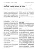
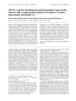
Start and stop codon classifier accuracy increases as informants are addedFigure 1
Start and stop codon classifier accuracy increases as informants
are added. The graph shows the generalization accuracy of
CONTRAST's start and stop codon classifiers as more informants are
added. The x-axis labels indicate the most recently added informant. For
example, at the point labeled 'chicken', the informant set consists of
mouse, opossum, dog and chicken.
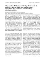
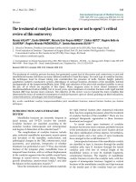
Splice site classifier accuracy increases as informants are addedFigure 2
Splice site classifier accuracy increases as informants are added.
The graph shows the generalization accuracy of CONTRAST's donor and
acceptor splice site classifiers as more informants are added. The x-axis
labels indicate the most recently added informant. For example, at the
point labeled 'chicken', the informant set consists of mouse, opossum, dog
and chicken.
0.7
0.72
0.74
0.76
0.78
0.8
0.82
0.84
armadillomacaqueratelephantrabbitcowtenrecchickendogopossummousehuman
Start Codon

Stop Codon
0.9
0.91
0.92
0.93
0.94
0.95
0.96
0.97
0.98
0.99

1
armadillomacaqueratelephantrabbitcowtenrecchickendogopossummousehuman
Donor Splice
Acceptor Splice
Table 3
Performance for human using EST evidence. Sensitivity (Sn) and
specificity (Sp) were evaluated at the gene, exon and nucleotide
levels and reported as percentages. Also shown are the average
number of genes and exons predicted for each cross-validation
fold. The column headings indicate the predictor and informants
used.
N-SCAN_EST
(mouse +
ESTs)
CONTRAST
(mouse +
ESTs)
CONTRAST

(11 informants
+ ESTs)
Gene Sn 46.8 60.7 65.4
Gene Sp 31.7 40.6 46.2
Exon Sn 89.7 92.6 93.9
Exon Sp 66.9 74.8 76.2
Nucleotide Sn 93.7 95.7 96.7
Nucleotide Sp 69.3 74.3 75.8
Genes predicted 23,339 23,787 22,507
Exons predicted 202,111 203,253 202,342
Genome Biology 2007, Volume 8, Issue 12, Article R269 Gross et al. R269.5
Genome Biology 2007, 8:R269
tors). As many genes in the ENCODE regions were well anno-
tated prior to EGASP, predictors of Categories 1 and 3 were at
a substantial advantage. For example, aligning RefSeq
mRNAs to the genome with BLAT produces a set of predic-
tions that is quite accurate (see Table 4).
CONTRAST's accuracy was significantly higher than the
other predictors in Category 4 at all levels of evaluation. The
average of CONTRAST's nucleotide sensitivity and specificity
was higher than any other predictor (regardless of category)
except for JIGSAW, an ensemble method that combines the
output of other predictors. CONTRAST's average exon level
performance was exceeded only by JIGSAW and the two pre-
dictors making use of PAIRAGON, a system for aligning
cDNAs to a genome. However, at the transcript and gene lev-
els, predictors that used expression data tended to show bet-
ter performance than CONTRAST.
The difference in CONTRAST's performance on the CCDS test
set and the EGASP test set are a consequence of the very

different compositions of the two sets. The CCDS set is known
to be fairly incomplete, containing only 16,008 genes of an
estimated 20,000-25,000. Nearly 90% of the genes in the
CCDS set have only one associated transcript, with an average
of 1.14 transcripts per gene. The GENCODE annotations used
a gold standard for EGASP so are believed to be much more
complete, and this idea is supported by the higher specifici-
ties observed for the EGASP test set. Furthermore, alternative
splice forms are very prevalent in the EGASP set, with 2.19
transcripts per gene on average. As CONTRAST does not
Table 4
Performance on the EGASP test regions. Sensitivity (Sn) and specificity (Sp) are shown at the nucleotide (Nuc), exon, transcript (Trans)
and gene levels for CONTRAST and the 19 predictors entered in the EGASP experiment. At each level of evaluation, the performance
of the predictor with the highest average sensitivity and specificity for a given category is shown in bold. Also shown is the performance
of the UCSC RefGene track, which consists of RefSeq cDNAs aligned to the genome. The track was evaluated just before the start of
the EGASP workshop.
Nuc Sn Nuc Sp Exon Sn Exon Sp Trans Sn Trans Sp Gene Sn Gene Sp
RefGene Track 85.34 98.50 73.23 94.67 41.91 75.21 77.03 82.56
Category 1 (any information)
AUGUSTUS-any 94.42 82.43 74.67 76.76 22.65 35.59 47.97 35.59
FGENESH++ 91.09 76.89 75.18 69.31 36.21 41.61 69.93 42.09
JIGSAW 94.56 92.19 80.61 89.33 34.05 65.95 72.64 65.95
PAIRAGON-any 87.77 92.78 76.85 88.91 39.29 60.34 69.59 61.32
Category 2 (target sequence)
AUGUSTUS-abinit 78.65 75.29 52.39 62.93 11.09 17.22 24.32 17.22
GENEMARK.hmm-A 78.43 37.97 50.58 29.01 6.93 3.24 15.20 3.24
GENEMARK.hmm-B 76.09 62.94 48.15 47.25 7.70 7.91 16.89 7.91
GENEZILLA 87.56 50.93 62.08 50.25 9.09 8.84 19.59 8.84
Category 3 (protein, mRNA, EST)
ACEVIEW 90.94 79.14 85.75 56.98 44.68 19.31 63.51 48.65

AUGUSTUS-EST 92.62 83.45 74.10 77.40 22.50 37.01 47.64 37.01
ENSEMBL 90.18 92.02 77.53 82.65 39.75 54.64 71.62 67.32
EXOGEAN 84.18 94.33 79.34 83.45 42.53 52.44 63.18 80.82
EXONHUNTER 90.46 59.67 64.44 41.77 10.48 6.33 21.96 6.33
PAIRAGON+NSCAN_EST 87.56 92.77 76.63 88.95 39.29 60.64 69.59 61.71
Category 4 (genomic alignments)
CONTRAST 94.44 89.25 77.68 86.02 25.12 47.87 53.04 47.87
AUGUSTUS-dual 88.86 80.15 63.06 69.14 12.33 18.64 26.01 18.64
DOGFISH 64.81 88.24 53.11 77.34 5.08 14.61 10.81 14.61
MARS 84.25 74.13 65.56 61.65 15.87 15.11 33.45 24.94
NSCAN 85.38 89.02 67.66 82.05 16.95 36.71 35.47 36.71
SAGA 52.54 81.39 38.82 50.73 2.16 3.44 4.39 3.44
Genome Biology 2007, 8:R269
Genome Biology 2007, Volume 8, Issue 12, Article R269 Gross et al. R269.6
predict alternative splicing if two exon annotations overlap, it
is able to make a correct prediction for at most one of the two.
This may explain why CONTRAST's exon sensitivity was
measured at only 77.7% with respect to the EGASP test set,
which contained many overlapping exons, but well over 90%
with respect to the CCDS test set, which contained few. This
explanation would require CONTRAST to preferentially pre-
dict splice forms present in the CCDS annotation over those
not present. We speculate that splice forms in the CCDS set
may have characteristic properties that set them apart from
alternative splice forms, such as a higher degree of conserva-
tion or stronger splice site signals.
Drosophila melanogaster gene prediction
To test how well CONTRAST performs on genomes distant
from human, we generated predictions for the April 2004
assembly of the Drosophila melanogaster genome (BDGP

Release 4/UCSC dm2). We used UCSC alignments of RefSeq
mRNAs to the Drosophila melanogaster genome as our set of
known genes. The set was filtered to remove annotations
likely to contain errors. In particular, we discarded annota-
tions containing in-frame stop codons, coding regions with a
length not divisible by three or splice sites not matching an
established consensus ('GT', 'GC' or 'AT' for donor sites, 'AG'
or 'AC' for acceptor sites). After filtering, the known gene set
contained 10,891 genes and 16,604 transcripts. The genomic
alignments we used came from a MULTIZ multiple alignment
of 12 Drosophila species and 3 additional insects (mosquito,
honeybee and red flour beetle). We used all 13 informants
from the alignment: Drosophila simulans (droSim1), Dro-
sophila sechellia (droSec1), Drosophila yakuba (droYak2),
Drosophila erecta (droEre2), Drosophila ananassae
(droAna3), Drosophila pseudoobscura (dp4), Drosophila
persimilis (droPer1), Drosophila willistoni (droWil1), Dro-
sophila virilis (droVir3), Drosophila mojavensis (droMoj3),
Drosophila grimshawi (droGri2), Anopheles gambiae
(anoGam1), Apis mellifera (apiMel2) and Tribolium casta-
neum (triCas2).
We again compared CONTRAST with N-SCAN, the most
accurate previous system for de novo prediction in Dro-
sophila melanogaster [6]. We used a four-fold cross-valida-
tion procedure as in the previous experiments. Table 5 shows
the accuracy of CONTRAST using all 13 informants, its accu-
racy using the best single informant (Drosophila ananassae)
and the accuracy of N-SCAN using Drosophila yakuba, Dro-
sophila pseudoobscura and A. gambiae as informants. The
N-SCAN predictions we used were taken from the UCSC

genome browser and represent the most accurate result for
N-SCAN (Randall Brown and Michael Brent, personal com-
munication). In contrast to the case for human gene
prediction, the availability of multiple informants increases
N-SCAN's accuracy on Drosophila melanogaster. However,
CONTRAST performs better even when using only one
informant. Furthermore, its accuracy improves significantly
with the addition of the other 12 informants.
Availability of predictions and software
Gene predictions for the human and Drosophila mela-
nogaster genomes, as well as source code for our implemen-
tation of CONTRAST, are available on the CONTRAST web
site [31]. We are currently in the process of generating predic-
tions for many other genomes, which will appear on the web
site and as custom tracks for the UCSC genome browser.
Discussion
Evaluating gene predictors
It is important to remember that comparing the performance
of gene predictors is not a completely straightforward propo-
sition. When evaluating a predictor, we are primarily inter-
ested in estimating how accurately it can identify unknown
genes. In practice, this is usually accomplished by training the
predictor on a portion of a set of known genes and then eval-
uating its performance on the remainder of the set. We can
trust such an estimate as far as we are willing to assume that
the predictor is as good at predicting unknown genes as it is
at predicting known genes. This assumption is violated for
predictors based on expression data, because we expect unan-
notated genes to be associated with fewer and lower-quality
expressed sequences than known genes. It is also reasonable

to expect that in fairly well-annotated organisms such as
human and Drosophila melanogaster, unannotated genes
may differ on average from annotated genes in terms of
properties such as degree of conservation, length and number
of exons.
In addition, the choice of annotation set to use for training
and evaluation can have a significant effect on the measured
accuracy of a predictor, as evidenced by the differences in
CONTRAST's performance on the EGASP and CCDS sets. In
particular, it is becoming clear that alternative splicing is
extremely prevalent in mammalian genomes, yet annotation
sets such as RefSeq and CCDS typically contain only one tran-
Table 5
De novo gene prediction performance for Drosophila mela-
nogaster. Sensitivity (Sn) and specificity (Sp) were evaluated at
the gene, exon and nucleotide levels and reported as percent-
ages. Also shown are the average number of genes and exons pre-
dicted for each cross-validation fold. The column headings
indicate the predictor and informants used.
N-SCAN
(3 informants)
CONTRAST
(Drosophila
ananassae)
CONTRAST
(13 informants)
Gene Sn 59.7 63.1 66.1
Gene Sp 46.4 48.3 52.7
Exon Sn 79.8 81.2 82.4
Exon Sp 67.9 71.6 74.2

Nucleotide Sn 96.2 96.3 96.9
Nucleotide Sp 79.4 82.4 83.4
Genome Biology 2007, Volume 8, Issue 12, Article R269 Gross et al. R269.7
Genome Biology 2007, 8:R269
script for most genes. The results we have presented should
be interpreted with these considerations in mind.
Design philosophy
In this work we have focused mainly on de novo gene recog-
nition. Accurately predicting the structure of a gene in a de
novo manner (that is, from genomic sequence alone) is a
much more difficult problem than making a prediction based
on expressed sequences. For example, if a high-quality, full-
length cDNA is available for a particular gene, it is a relatively
simple matter to align the cDNA back to the genome and thus
recover the exon-intron structure of one of the gene's tran-
scripts. In the absence of a full-length cDNA, genes well cov-
ered by EST alignments can be predicted accurately by
merging overlapping ESTs to form a complete gene structure.
The vast majority of known genes have been discovered by
randomly sequencing cDNA libraries to obtain a large
number of expressed sequences and then applying expres-
sion-based prediction methods. However, this approach has
its limits. Genes expressed at low levels or with highly
restricted patterns of expression may escape even a very deep
level of sequencing. This appears to be the case for a signifi-
cant fraction of human and mouse genes: results from the
Mammalian Gene Collection project show that random
sequencing methods reach saturation long before a complete
set of genes can be recovered [29]. For genes whose full struc-
ture cannot be determined based on expression evidence

alone, we must rely on other methods to complete the anno-
tation. The most promising option is the targeted experimen-
tal validation of computational predictions using RT-PCR
[32-34]. These predictions need not be purely de novo, as
incorporating EST alignments can help guide predictions on
genes with partial EST coverage. However, the accuracy of the
predictions on genes or parts of genes not covered by ESTs
will depend on our ability to recognize gene structures from
genomic sequence. These considerations explain the design
philosophy behind CONTRAST, which was intended to be a
highly accurate de novo predictor with the additional capabil-
ity of incorporating EST evidence when available. Large-scale
projects aiming to identify new genes through the experimen-
tal confirmation of de novo predictions have already met with
considerable success. For example, thousands of novel
human exons predicted by N-SCAN and not covered by any
EST alignments have been verified by RT-PCR experiments
(Computational prediction and experimental validation of
novel human genes for the mammalian gene collection, Siepel
et al, in preparation). Such projects will benefit greatly from
increases in the accuracy of de novo gene prediction.
Discriminative approach
As we have shown, CONTRAST achieves a substantial
increase in performance over previous de novo predictors in
the human and Drosophila melanogaster genomes. The fact
that CONTRAST performs well on both of these distantly
related species suggests that similar results will hold for a
variety of higher eukaryotes. We believe a key factor in CON-
TRAST's success is the unique way in which it uses alignment
information to make predictions. Previous predictors (for

example, N-SCAN, ExoniPhy, EvoGene and DOGFISH) have
integrated information from multiple alignments through the
use of evolutionary models that define a probability distribu-
tion over alignment columns. These models use independ-
ence assumptions derived from a phylogenetic tree to factor
the high-dimensional joint distribution over all of the charac-
ters in a column into a product of distributions involving at
most two characters each. To facilitate this, hidden variables
corresponding to the value of ancestral characters are intro-
duced. Gene predictors that use multiple alignments typically
contain many of these models, each one corresponding to a
particular annotation of the target species character (for
example, coding, intronic or intergenic). The use of evolution-
ary models has been necessitated by the fact that previous
gene predictors have been based on some variation of a hid-
den Markov model (HMM). HMMs are generative models,
meaning they define a joint distribution over their input data
and a labeling of that data. Thus, HMM-based gene predictors
are obligated to model multiple alignments explicitly if they
wish to use them as input.
Instead of learning to model the properties of different types
of alignment columns and then using these models to predict
genes, CONTRAST attempts to learn parameters that approx-
imately maximize the accuracy of its boundary classifiers and
global gene model. This type of approach is known as dis-
criminative. Discriminative methods have been shown to
outperform generative approaches in a wide variety of set-
tings [35-39]. CONTRAST uses SVMs for its coding boundary
classifiers and a CRF for its global model of gene structure.
Both models directly use features of the multiple alignment

without postulating hidden ancestral characters or making
assumptions about evolutionary relationships.
Relationship to previous work
A first attempt to use CRFs for gene prediction was described
in [40]. The authors show that a CRF-based gene predictor
outperforms a HMM-based predictor, GENIE [41], when
both predictors use protein alignments. However, GENIE
performs better in de novo prediction experiments and no
comparisons with more accurate de novo predictors such as
N-SCAN were made.
Two more recent studies have also addressed the issue of
using discriminative methods for de novo gene prediction. In
the first study, the authors introduce CRAIG, an ab initio
gene predictor based on a semi-Markov CRF [2]. CRAIG does
not make use of alignment information, but instead uses a
rich set of target sequence features. CRAIG reaches a signifi-
cantly higher level of accuracy than other ab initio predictors,
which are based on generative models. Although its overall
performance is not on a par with the best de novo predictors
[2,17], the fact that CRAIG makes predictions without using
alignments means it is well suited for discovering rapidly
Genome Biology 2007, 8:R269
Genome Biology 2007, Volume 8, Issue 12, Article R269 Gross et al. R269.8
evolving genes. The second study describes Conrad [42], an
alignment-based gene predictor that takes a partially discrim-
inative approach. Conrad uses a semi-Markov CRF to com-
bine output from generative evolutionary models with non-
probabilistic features based on alignment gap patterns and
EST evidence. Conrad has been shown to outperform TWIN-
SCAN on a fungal genome, but has not been applied to the

more difficult task of predicting genes in a large genome with
long introns. We were not able to test Conrad on the human
or Drosophila melanogaster genomes as its current imple-
mentation does not support the parallelization of training
computations across a compute cluster, making training on
large genomes prohibitively expensive [43].
The two-stage approach used in CONTRAST, in which coding
region boundary classifiers are separated from a global model
of gene structure, is similar to the strategy employed by DOG-
FISH. There are three principal differences between the two
methods. First, the classifiers used by DOGFISH consider a
much larger window around potential coding boundaries,
including up to 100 positions in the coding region. In CON-
TRAST, at most six coding positions are considered by a clas-
sifier; most of the task of scoring coding sequence is left to the
global model. Second, DOGFISH's classifiers combine scores
from generative models, such as phylogenetic evolutionary
models and position-specific scoring matrices, whereas the
classifiers used by CONTRAST take only the alignment itself
as input. Finally, DOGFISH's global model is a generatively
trained HMM, while CONTRAST uses a CRF trained to max-
imize expected coding region boundary accuracy.
In many ways, CONTRAST is less complex than other leading
de novo gene predictors. Most predictors are based on a
model that allows for semi-Markov dependencies between
labels, such as a generalized HMM or a semi-Markov CRF;
the fact that CONTRAST uses a standard CRF means its mod-
els of exon and intron lengths are fairly restricted. Moreover,
CONTRAST does not explicitly model promoters, untrans-
lated regions or conserved non-coding regions. Finally, the

feature set used in CONTRAST is relatively simple: it contains
no features designed to detect splicing branch points, polya-
denylation signals or signal peptide sequences, for example.
Incorporating more sophisticated biological models would
likely improve predictive accuracy and is an important direc-
tion for future work. Other possible extensions to the system
include adding the ability to predict untranslated regions,
alternative splicing or overlapping genes.
Conclusion
The failure of multiple alignment-based gene predictors to
improve upon single informant performance in human has
been a puzzling phenomenon. The situation runs counter to
the strong intuitive feeling that additional genomes should
provide enough extra statistical power to significantly
increase predictive accuracy. At least one researcher was
prompted to speculate that the lack of success could be a
result of inadequate alignment quality or insufficient cross-
species conservation of gene structure [30]. Our results sug-
gest that the necessary information has been present in the
alignments all along, but new methods were needed to effec-
tively make use of it.
The greater precision of de novo gene prediction has two
important consequences. First, better predictions should
expedite efforts to verify the complete set of protein coding
genes in human and other organisms experimentally. Tar-
geted experiments designed to validate novel predictions will
be able to recover more genes and operate at a higher effi-
ciency than previously possible. Second, de novo predictions
are becoming accurate enough that they can be relied upon
with reasonable confidence. At present, testing computa-

tional predictions experimentally on a genome-wide scale is a
time-consuming process. For many genomes, de novo predic-
tions will provide an important annotation resource until
annotation to a more exacting standard can be completed.
Materials and methods
Global model of gene structure
CONTRAST uses a CRF for its global model of gene structure.
The CRF assigns a probability to each possible labeling y of a
set of input data x. For our purposes, x consists of a genomic
sequence from the target organism along with alignments
from informant genomes and (optionally) ESTs, while y
encodes a set of possible locations and structures of the genes
in x.
Part of a typical set of input dataFigure 3
Part of a typical set of input data. The input data consists of 13 rows.
The first row contains sequence from the target genome, the second to
twelfth rows contain aligned sequence from informant genomes and the
last row encodes information about the alignments of ESTs to the target
genome.
human ACAGGTGAGGAGGCG
macaque
mouse
rat ACAGGTGAGAAAG
rabbit
dog ACAGGTGAGGAGTCG
cow ACAGGTGAGCAGTCG
armadillo ACAGGTGAGGAG_CA
elephant
tenrec
opossum CCAGGGAAG

chicken CCAGGTGA
EST SSSSIIIIIIIIIII
Genome Biology 2007, Volume 8, Issue 12, Article R269 Gross et al. R269.9
Genome Biology 2007, 8:R269
Figure 3 shows part of a typical input to CONTRAST. The first
row is the DNA sequence from the target genome. This row
can contain characters corresponding to the four DNA bases
as well as 'N'. Masked positions are indicated by lowercase
letters. The next 11 rows are alignments from a variety of
other species. These rows can contain the same characters as
the first row, plus '_' for a gap in the alignment and '.' for una-
ligned positions. The final row contains a sequence which
encodes information about EST alignments to the target
genome. This row can contain five characters: 'N' for posi-
tions not covered by an EST alignment, 'S' for positions which
all spliced EST alignments indicate to be in an exon, 'I' for
positions which all spliced EST alignments indicate to be in
an intron, 'C' for positions which some spliced EST align-
ments indicate to be an exon and some an intron and 'U' for
positions covered by only unspliced EST alignments.
Figure 4 illustrates the structure of labelings in CONTRAST.
Nodes in the diagram represent possible labels for a single
position in the input data. Two labels are allowed to occur in
succession only if there is an arrow from the first label to the
second. Thus, a valid labeling corresponds to a path through
the diagram. Labels for the coding sequence, shown as red
nodes, are classified as either belonging to a gene with a single
coding exon or to the initial, internal or terminal coding exon
of a multi-exon gene. There are three labels (1, 2 and 3) for
each exon type, corresponding to whether the position is the

first, second or third base of a codon. Coding region bounda-
ries correspond to neighboring labels of different colors. Each
coding region boundary in the labeling must occur at a posi-
tion with a valid consensus sequence in the target genome
('ATG' for start codons; 'TAA', 'TAG' or 'TGA' for stop codons;
'GT' or 'GC' for donor splice sites; and 'AG' for acceptor splice
sites). The exon and intron labels in the diagram represent
genes on one DNA strand only; the full model contains a sym-
metric set of labels (not shown) representing genes on the
opposite strand. The full model also includes additional
intron labels to track stop codons that are split across exons.
For example, on the positive strand, the 'Intron 1' label is split
into two labels, one for introns bordered on the 5' end by a
coding 'T' and one for all other introns. Similarly, the 'Intron
2' label is split into three labels, depending on whether the
previous two coding bases were 'TA', 'TG' or neither. These
additional labels serve to disallow labelings containing genes
with split in-frame stop codons.
The conditional probability of a labeling y given a sequence x
is defined as
where w, the weight vector, is learned from training data and
F(x, y), the summed feature vector, is given by
Here L is the length of the input data (and labeling), y
i
is the
label at position i and f, called the feature mapping, is a vec-
tor-valued function which determines the information used
to calculate the score of a position. The components of f are
referred to as the CRF's features. For simplicity, we assume
the existence of a special initial label y

0
.
Specifying f is the key task in designing a CRF. A few entries
in the feature mapping for a simple CRF-based gene predictor
are given as follows:
Here 1{} is the indicator function, which returns 1 if its argu-
ment is true and 0 otherwise. In this example, a position
receives a score of w
1
if the label at the previous position is
'Intron' and the label at the current position is 'Exon', plus a
score of w
2
if the label at the current position is 'Exon' and the
corresponding position in the sequence contains a 'G'. The
score of a labeling, w
T
F(x, y), is simply the sum of the scores
of all of its positions. The probability of a labeling is obtained
by exponentiating its score and dividing by a normalizing
constant which ensures that the probabilities of all labelings
sum to one.
Feature mapping
The feature mapping used in CONTRAST consists of three
main types of features: features that score transitions
between labels, features that score a label based on sequence
near its position and features that score coding region
boundaries.
Transition features are defined as follows. For each pair of
labels y and y' such that y is allowed to follow y', the feature

mapping contains the following element:
f(y
i-1
, y
i
, i, x) = 1{y
i-1
= y' and y
i
= y}.
There are three types of sequence-based features: features
based on the target sequence, features based on the alignment
of a particular species to the target sequence and features
based on EST evidence. Figure 5 provides a graphical illustra-
tion of the three feature types, which we describe in detail in
the following. Let S
intron
denote the set of candidate labels cor-
responding to intronic positions in a forward-strand gene of
the target sequence and, similarly, let S
exon1
, S
exon2
and S
exon3
denote sets of labels corresponding to the three forward-
strand coding frames, respectively. For example, S
exon1
=
{'Initial Exon 1', 'Internal Exon 1, 'Terminal Exon 1', 'Single

P
e
e
(|)
(,)
(, )
,yx
wFxy
wFxy
y
=
′
′
∑
T
T
Fxy f x(,) ( , ,,).=
−
=
∑
yyi
ii
i
L
1
1
fx(,,,)
{}
{yyi
yy

yx
ii
ii
ii−
−
=
==
==
1
1
1
1
Intron and Exon
Exon and

’’ ’ } .G
"
⎡
⎣
⎢
⎢
⎢
⎤
⎦
⎥
⎥
⎥
Genome Biology 2007, 8:R269
Genome Biology 2007, Volume 8, Issue 12, Article R269 Gross et al. R269.10
The structure of labelings in CONTRASTFigure 4

The structure of labelings in CONTRAST. Each node in the graph is a possible label for a single position in the target sequence. A labeling is legal if
it corresponds to a path through the graph.
Intergenic
Single
Exon 1
Single
Exon 2
Single
Exon 3
Initial
Exon 1
Initial
Exon 2
Initial
Exon 3
Intron 1 Intron 2 Intron 3
Internal
Exon 1
Internal
Exon 2
Internal
Exon 3
Terminal
Exon 1
Terminal
Exon 2
Terminal
Exon 3
Genome Biology 2007, Volume 8, Issue 12, Article R269 Gross et al. R269.11
Genome Biology 2007, 8:R269

Exon 1'}. We refer to each of these four label sets as forward
strand label sets and define their reverse strand counterparts
Ŝ
intron
,
Ŝ
exon1
,
Ŝ
exon2
, and
Ŝ
exon3
analogously.
For each DNA hexamer h and forward strand label set S, the
feature mapping contains
where x
r,i:j
are the characters in row r of the input data from
positions i to j inclusive and is the reverse complement of
h. Defining the features in this way ensures that a specific
hexamer will be treated the same whether it is part of a gene
on the forward or reverse strand. Additional features are
included to score hexamers in the target sequence that con-
tain an 'N':
1{(y
i
∈ S and x
1,i:i+5
contains 'N') or

(y
i
∈
Ŝ
and x
1,i-5:i
contains 'N'}.
Finally, masked positions, which are indicated in the target
sequence by lowercase characters, are scored using a set of
features of the form:
1{(y
i
∈ S or y
i
∈
Ŝ
) and x
i
is lowercase}.
Thus, each label (other than 'Intergenic') has 4,098 target
sequence features associated with it: one for each possible
hexamer consisting of only DNA bases, one for all hexamers
containing an 'N' and one for masked positions.
Alignment sequence features are based on the combination of
a trimer in the target sequence and a trimer in one of the
aligned sequences. For each forward strand label set S, row r
of the input data corresponding to an informant alignment
and pair of DNA trimers t and t', the feature mapping contains
For aligned trimers containing gaps but no unaligned charac-
ters, the feature mapping takes into account only the configu-

ration of gaps in the trimer and ignores any DNA base
characters. This is accomplished through use of the concept of
a gap pattern. A gap pattern is a string consisting of the char-
acters '_' and 'X'. A string s matches a gap pattern g if s con-
tains a '_' character at every position that g does and a DNA
base character at every position that g has an 'X'. For exam-
ple, the strings 'A_G', 'C_T' and 'A_A' all match the gap pat-
tern 'X_X'. For each forward strand label set S, alignment row
r and possible three-character gap pattern g except 'XXX', the
feature mapping contains
Features that score a label based on local sequenceFigure 5
Features that score a label based on local sequence. CONTRAST contains three types of features for scoring a label based on local sequence:
features based on hexamers in the target sequence (shown in blue), features based on a trimer in the target sequence and a trimer in an informant
alignment (shown in red) and features based on a position in the EST sequence (shown in green).
human ACAGGTGAGGAGGCG
armadillo ACAGGTGAGGAG_CA
EST SSSSIIIIIIIIIII
EST sequence feature
All spliced EST alignments indicate intron
Target sequence feature
Hexamer AGGTGA
Alignment sequence feature
Armadillo, gap pattern X_X
1
15 15
{( ) (
ˆ
)},
,: , :
yS x h yS x h

iii iii
∈=∈=
+−
and or and



h
1
12 2 1
{( ) (
ˆ
,: ,: ,
yS x t x t yS x
iii rii i
∈==
′
∈
++
and and or and

iii rii
tx t
−−
==
′
22:,:
)}.




and
Genome Biology 2007, 8:R269
Genome Biology 2007, Volume 8, Issue 12, Article R269 Gross et al. R269.12
where s
R
indicates the reversal of string s. Finally, trimers
containing unaligned characters are divided into three
groups: those representing the start of an alignment (' X' and
'.XX'), those representing the end of an alignment ('X ' and
'XX.') and those that are completely unaligned (' '). Here, 'X'
is interpreted as meaning any character other than '.'. For
each such group g, forward strand label set S and alignment
row r, the feature mapping contains
EST sequence features are the most straightforward. For each
forward strand label set S and EST sequence character e, the
feature mapping contains
1{(y
i
∈ S or y
i
∈
Ŝ
) and x
est,i
= e},
where x
est,i
is the EST sequence character at position i.
Features for scoring coding region boundaries using align-

ment information are based on outputs from a set of binary
classifiers. Each boundary type (start codon, stop codon, GT
donor splice, GC donor splice and acceptor splice) has an
associated classifier. The classifier takes as input a small win-
dow around two neighboring positions in the alignment
potentially corresponding to a boundary and outputs a deci-
sion value. Large positive decision values indicate a confident
prediction that the positions in question do in fact constitute
a boundary of the classifier's type, highly negative values indi-
cate a confident negative prediction and values near zero indi-
cate an uncertain prediction. We chose not to directly use the
classifier's decision value as a feature, because this would
result in the score of a boundary being a simple linear
function of the classifier's output. To allow for a more general
relationship, CONTRAST maps the output of a classifier to a
score using a piecewise linear function interpolated through a
set of control points. More precisely, the score of a decision
value d is given by
where (x
i
, w
i
) and (x
i+1
, w
i+1
) are control points selected such
that d ∈ [x
i
, x

i+1
] if possible or the two points with x-coordi-
nates closest to d if not. The number of control points and
their x-coordinates are fixed before CRF training (see the
training procedure section), while the w-coordinates of the
control points are learned by the CRF (that is, they corre-
spond to components of the weight vector w). This is accom-
plished by specifying the feature mapping such that it
contains one feature for each control point (x
i
, w
i
) associated
with a particular classifier. Each such feature has non-zero
value only if the labels (y
i-1
, y
i
) correspond to a boundary of
the classifier's type and the classifier's score at position i is
such that (x
i
, w
i
) is used as a control point to determine the
CRF score. In that case, the feature's value is equal to the
interpolation coefficient of its associated control point: (1 - c)
if it is the control point with the lower x-coordinate and c oth-
erwise.
CONTRAST also includes features that score coding region

boundaries based on EST sequence. For each coding region
boundary type b and pair of EST sequence characters e and e',
the feature mapping contains
1{(y
i-1
, y
i
) corresponds to b, x
est,c
= e and x
est,nc
= e'}.
Here, x
est,c
is the EST sequence character at the coding posi-
tion closest to the boundary, while x
est,nc
is the EST sequence
character at the non-coding position closest to the boundary.
Figure 6 provides an illustration of the two types of feature
that score coding region boundaries.
Coding region boundary classifiers
CONTRAST uses SVMs as its coding region boundary classi-
fiers. We use a set of binary features to define a one-to-one-
mapping from the space of multiple alignment windows to
the space of SVM input vectors. For each possible character c,
row i and column j in the window, the SVM feature vector
contains an element
1{the character in row i and column j is c}.
We use quadratic kernels for the SVMs, allowing them to

operate implicitly in a much larger feature space. For each
pair of features f
i
and f
j
in the original space, the expanded
feature space contains the feature f
i
f
j
. As f
i
and f
j
are binary
features, f
i
f
j
is also a binary feature whose argument is the
conjunction of the arguments to f
i
and f
j
. An example feature
in the expanded space is
1{the character in position 4 of the 'mouse' row is 'G'
and the character in position 5 of the 'rat' row is 'T'}.
Table 6 lists the window sizes and positions for the five
boundary classifiers used in CONTRAST, along with the posi-

tion of a required consensus sequence. The coordinates in the
table are defined such that 1 is the position immediately 3' of
the coding region boundary, -1 is the position immediately 5'
of the boundary and coordinates increase in the 5' to 3'
direction.
Maximum boundary accuracy decoding
The standard procedure for using a CRF to predict labels for
a new sequence involves selecting the labeling with the maxi-
mum conditional likelihood given the sequence,
1
22
{( ) (
ˆ
,: , :
yS x g yS x
irii irii
∈∈
+−
and matches or and ma
R
ttches
R
g )},
1
22
{( ) (
ˆ
)}.
,: , :
yS x g yS x g

irii irii
∈∈∈∈
+−
and or and
RR
sd cw cw
c
dx
i
x
i
x
i
ii
() ( ) ,
,
=− +
=
−
+
−
+
1
1
1
Genome Biology 2007, Volume 8, Issue 12, Article R269 Gross et al. R269.13
Genome Biology 2007, 8:R269
Features that score coding region boundariesFigure 6
Features that score coding region boundaries. CONTRAST contains two types of feature for scoring coding region boundaries. The first, shown in
red, maps the output of a classifier to a score using a piecewise linear function learned during CRF training. In this example, the score from the GT splice

donor classifier falls between the fourth and fifth control points for the function, with interpolation coefficients of 0.312 and 0.688. The second type of
feature, shown in green, scores a coding region boundary based on the EST sequence characters that flank it.
human ACAGGTGAGGAGGCG
macaque
mouse
rat ACAGGTGAGAAAG
rabbit
dog ACAGGTGAGGAGTCG
cow ACAGGTGAGCAGTCG
armadillo ACAGGTGAGGAG_CA
elephant
tenrec
opossum CCAGGGAAG
chicken CCAGGTGA
EST SSSSIIIIIIIIIII
EST splice donor feature
All spliced EST alignments indicate exon boundary
GT splice donor classifier score
1.754
Splice donor classifier feature
Control points 4 and 5, coefficients 0.312 and 0.688
Genome Biology 2007, 8:R269
Genome Biology 2007, Volume 8, Issue 12, Article R269 Gross et al. R269.14
Instead, we select the labeling that maximizes a weighted dif-
ference between the expected number of true-positive and
false-positive coding region boundary predictions:
Here, B is the set of all pairs of labels corresponding to a cod-
ing boundary and
κ
is a constant that controls a tradeoff

between sensitivity and specificity. We used
κ
= 1 for the
human experiments.
For the Drosophila melanogaster experiments, we chose
κ
=
1.5 after observing that this higher value of
κ
led to slightly
better performance.
We can efficiently compute y by first running the forward and
backward algorithms to calculate the posterior probabilities
of all pairs of adjacent labels, and then running a Viterbi-like
dynamic programming algorithm to find the optimal labeling.
Maximum expected boundary accuracy training
Standard algorithms for training a CRF are based on maxi-
mum conditional likelihood. Given a set of training examples
, conditional likelihood training finds
weights for the CRF that maximize the conditional likelihood
of the training data,
Instead, we optimize the expected boundary accuracy on the
training set, which we define as
Informally, EBA(w) is the weighted sum of the probabilities
of all correct coding boundary labels and the negative proba-
bilities of all possible incorrect coding boundary labels. Note
that the training data may contain coding boundaries from
unannotated genes, which will be penalized as incorrect. In
such cases, a relatively high value of
λ

may be required to off-
set spurious penalties. We used
λ
= 15 for all experiments.
The choice to use maximum expected boundary accuracy
training for CONTRAST was motivated by a previous result
demonstrating that a training criterion based on maximum
accuracy led to far better performance than maximum condi-
tional likelihood training for a gene prediction task [44].
In practice, we optimize EBA(w) using a gradient-based opti-
mization algorithm (described in the following). The gradient
can be calculated efficiently using a dynamic programming
algorithm that is only a small constant factor slower than the
algorithm used to compute the gradient of L(w). The
techniques used are very similar to those described previously
[44]; we omit the details for reasons of brevity.
Cross-validation procedure
The cross-validation procedure we used was designed to esti-
mate CONTRAST's ability to discover unannotated genes
when trained on and used to generate predictions for an
entire genome. We divided the annotations of known genes
into four sets at random. At each iteration of the cross-valida-
tion procedure, we trained CONTRAST using only annota-
tions from three of the four sets. We then generated
predictions for the full genome and counted the number of
correctly predicted nucleotides, exons and genes not included
in the training set. The results for each iteration were
summed to calculate the total number of correct predictions.
To determine specificity, we considered the number of
predictions made by CONTRAST to be the average of the

number of predictions made at each iteration.
Training procedure
To train CONTRAST, we first split the target genome into
fragments of length 1 Mbp. The fragments were then ran-
domly divided into three sets: 25% went into a set used for
SVM training, 50% went into a set used to train the CRF and
the remaining 25% formed a holdout set used to estimate gen-
eralization accuracy.
Table 6
Coding region boundary classifiers. Coding region boundary clas-
sifiers. Window sizes and positions are shown for the five coding
region boundary classifiers used by CONTRAST. Coordinates are
defined such that the boundary occurs between the adjacent posi-
tions -1 and 1 (that is, either position -1 is coding and position 1 is
coding or the reverse is true), with coordinates increasing in the
5' to 3' direction. Each classifier's require consensus sequence is
shown in the second column.
Consensus 5' end 3' end Length
Start codon A
1
T
2
G
3
-8 6 14
Stop codon T
1
A
2
A

3
, T
1
A
2
G
3
, T
1
G
2
A
3
166
Donor splice GT G
1
T
2
-3 8 11
Donor splice GC G
1
C
2
-3 8 11
Acceptor splice A
-2
G
-1
-27 3 30
yyx

y
=
′
′
arg max ( | ).P
y
y
=
′′
∈
′′
′′
=
′
−
=
−
−
∑
arg max {( , ) } ( , ),
(,)
1
1
2
1
1
yy BAyy
Ay y
j
j

L
jjj
jj
κ
PPy y Py y
jj jj
( , | ) ( ( , | )).
′′
−−
′′
−−11
1xx
 =
=
{,}
() ()
xy
tt
t
m
1
LP
tt
t
m
() ( | ).
() ()
wyx=
=
∏

1
EBA( ) ,
{( , ) } (
()
() () () (
w =
=∈
==
−−
∑∑
A
AyyBPy
j
t
j
L
t
m
j
t
j
t
j
t
j
t
21
11
1
λ

tt
j
tt
jj
t
yyByy
yPyy
jj
j
t
j
)()() ()
(,)(,
,|) (,|)
()
xx−
′′
−
′′
∈−
−
−
1
1
1
(()
)
.
t
∑

Genome Biology 2007, Volume 8, Issue 12, Article R269 Gross et al. R269.15
Genome Biology 2007, 8:R269
As CONTRAST predicts only one transcript per gene, we used
only one randomly selected transcript of each gene for
training.
For each example of a particular type of coding region bound-
ary that occurs in the SVM training set, we created a positive
training example for the appropriate SVM. We also created a
negative example by searching, in a randomly selected
direction, for the nearest occurrence of the SVM's required
consensus in the target sequence. We chose this method of
selecting negative examples over simply sampling uniformly
from the target genome for two reasons. First, negative exam-
ples taken from positions near a true coding boundary display
a relatively high level of conservation, making them difficult
to classify. Second, these negative examples correspond to
plausible mispredictions in which a coding boundary is pre-
dicted slightly 5' or 3' of its true location. We also extracted a
second set of positive and negative examples by applying the
above procedure to the CRF training set. This set was
reserved for estimating the generalization performance and
was not used directly in SVM training. After the SVM exam-
ples were constructed, we trained standard two-class SVMs
using code from the libsvm library [45]. The slack variable
coefficient C was selected to maximize classification accuracy
on the examples from the CRF training set.
After SVM training was complete, we set the abscissas of the
control points used to map SVM decision values to CRF
scores. For each SVM, the outermost two abscissas were
selected such that they bracketed 99% of the decision values

for positive examples in the CRF training set. The remaining
abscissas were placed at uniform intervals between those two.
Ten control points were used for the GT donor splice and
acceptor splice classifiers; the other classifiers used five con-
trol points. An initial CRF weight vector w was then com-
puted as follows. Weights for transition features were set
according to the formula
Here w
ij
is the weight for a transition from label i to label j, N
i
is the number of times label i appeared in the CRF training set
and N
ij
is the number of times label j appeared immediately
after label i in the CRF training set. Weights corresponding to
the ordinates of control points were set according to the
formula
Here w
i
is the ordinate of control point i, P
i
is the number of
positive examples in the CRF training set with a decision
value such that i would be used to compute its CRF score and
N
i
is the corresponding number for negative examples. The
remaining weights were set to small random values chosen
uniformly from the interval [-10

-3
, 10
-3
]. The process of select-
ing an initial weight vector should not be interpreted as a
parameter estimation procedure, as the final CRF weights
bear little resemblance to their initial values. Rather, the
above procedure serves to initialize the CRF learning algo-
rithm at a reasonable starting point.
Finally, the weight vector was optimized to maximize the
function
Here the first term is the expected boundary accuracy for the
CRF training set (explained previously), while the second is a
regularization term added to combat overfitting.
The sum in the regularization term is over weights for hex-
amer and trimer pair features only. The other weights were
not subject to regularization, because their associated fea-
tures occurred often enough in the training data that overfit-
ting was not a significant problem.
The Rprop algorithm was used for optimization [46]. We did
not run Rprop to convergence, but rather applied an early
stopping procedure: optimization was terminated if five iter-
ations occurred without an improvement in the value of the
expected boundary accuracy for the holdout set. The regular-
ization constant C was selected by performing a golden sec-
tion search [47] to determine which value led to the best
expected boundary accuracy for the holdout set. Training
CONTRAST on the human genome with 11 informants
required approximately 12 hours using 200 Intel Xeon E5345
processors (2.33 GHz) in parallel.

Acknowledgements
We thank Jeltje van Baren, Randall Brown and Michael Brent's computa-
tional genomics group for providing their latest N-SCAN and N-
SCAN_EST predictions. Thanks also go to Paul Flicek for performing the
evaluation of CONTRAST predictions on the EGASP test set. SSG and
CBD were supported by NDSEG fellowships.
References
1. Burge C, Karlin S: Prediction of complete gene structures in
human genomic DNA. J Mol Biol 1997, 268:78-94.
2. Bernal A, Crammer K, Hatzigeorgiou A, Pereira F: Global discrim-
inative learning for higher-accuracy computational gene
prediction. PLoS Comput Biol 2007, 3:e54.
3. Batzoglou S, Pachter L, Mesirov JP, Berger B, Lander ES: Human and
mouse gene structure: comparative analysis and application
to exon prediction. Genome Res 2000, 10:950-958.
4. Bafna V, Huson DH: The conserved exon method for gene find-
ing. Proceedings of the Eighth International Conference on Intelligent Sys-
tems for Molecular Biology 2000:3-12.
5. Korf I, Flicek P, Duan D, Brent MR: Integrating genomic hom-
ology into gene structure prediction. Bioinformatics 2001,
17(Suppl 1):S140-S149.
6. Gross SS, Brent MR: Using multiple alignments to improve
gene prediction. Proceedings of the Ninth Annual International Confer-
ence on Research in Computational Molecular Biology (RECOMB 2005)
w
N
ij
N
i
ij

=
⎛
⎝
⎜
⎜
⎞
⎠
⎟
⎟
log .
w
P
i
N
i
i
=
⎛
⎝
⎜
⎞
⎠
⎟
log .
EBA( ) .w −
∑
Cw
i
i
2

Genome Biology 2007, 8:R269
Genome Biology 2007, Volume 8, Issue 12, Article R269 Gross et al. R269.16
2005.
7. Alexandersson M, Cawley S, Pachter L: SLAM: cross-species gene
finding and alignment with a generalized pair hidden Markov
model. Genome Res 2003, 13:496-502.
8. Parra G, Agarwal P, Abril JF, Wiehe T, Fickett JW, Guigo R: Com-
parative gene prediction in human and mouse. Genome Res
2003, 13:108-117.
9. Pedersen JS, Hein J: Gene finding with a hidden Markov model
of genome structure and evolution. Bioinformatics 2003,
19:219-227.
10. Siepel A, Haussler D: Computational identification of evolu-
tionarily conserved exons. Proceedings of the Eighth Annual Interna-
tional Conference on Research in Computational Molecular Biology
(RECOMB 2004) 2004:177-186.
11. Carter D, Durbin R: Vertebrate gene finding from multiple-
species alignments using a two-level strategy. Genome Biol
2006, 7(Suppl 1):S6.
12. Arumugam M, Wei C, Brown R, Brent M: Pairagon+N-
SCAN_EST: a model-based gene annotation pipeline.
Genome Biol 2006, 7(Suppl 1):S5.
13. Wei C, Brent M: Using ESTs to improve the accuracy of de
novo gene prediction. BMC Bioinformatics 2006, 7:.
14. Birney E, Clamp M, Durbin R: GeneWise and Genomewise.
Genome Res 2004, 14:988.
15. Djebali S, Delaplace F, Crollius H: Exogean: a framework for
annotating protein-coding genes in eukaryotic genomic
DNA. Genome Biol 2006, 7(Suppl 1):S7.
16. Stanke M, Waack S: Gene prediction with a hidden Markov

model and a new intron submodel. Bioinformatics 2003, 19:2.
17. Guigo R, Flicek P, Abril J, Reymond A, Lagarde J, Denoeud F, Anton-
arakis S, Ashburner M, Bajic V, Birney E, Castelo R, Eyras E, Ucla C,
Gingeras T, Harrow J, Hubbard T, Lewis S, Reese M: EGASP: the
human ENCODE genome annotation assessment Project.
Genome Biol 2006, 7(Suppl 1):S2.
18. Cortes C, Vapnik V: Support-vector networks. Mach Learn 1995,
20(3):273-297.
19. Lafferty J, McCallum A, Pereira F: Conditional random fields:
probabilistic models for segmenting and labeling sequence
data. Proceedings of the Eighteenth International Conference on Machine
Learning 2001:282-289.
20. Siepel A, Haussler D: Combining phylogenetic and hidden
Markov models in biosequence analysis. Proceedings of the
Seventh Annual International Conference on Research in Computational
Molecular Biology 2003:277-286.
21. CCDS Report for Consensus CDS, 2007 [http://
www.ncbi.nlm.nih.gov/CCDS]
22. Blanchette M, Kent WJ, Riemer C, Elnitski L, Smit AF, Roskin KM,
Baertsch R, Rosenbloom K, Clawson H, Green ED: Aligning multi-
ple genomic sequences with the threaded blockset aligner.
Genome Res 2004, 14:708-715.
23. Wang M, Buhler J, Brent M: The effects of evolutionary distance
on TWINSCAN, an algorithm for pair-wise comparative
gene prediction. Cold Spring Harb Symp Quant Biol 2003,
68:125-130.
24. Karolchik D, Baertsch R, Diekhans M, Furey TS, Hinrichs A, Lu YT,
Roskin KM, Schwartz M, Sugnet CW, Thomas DJ: The UCSC
genome browser database. Nucleic Acids Res 2003, 31:51-54.
25. Smit AFA, Hubley R, Green P: RepeatMasker Open-3.0. [http://

www.repeatmasker.org].
26. Keibler E, Brent M: Eval: a software package for analysis of
genome annotations. BMC Bioinformatics 2003, 4:50.
27. Kent WJ: BLAT - The BLAST-like alignment tool. Genome Res
2002, 12:656-664.
28. Benson DA, Karsch-Mizrachi I, Lipman DJ, Ostell J, Wheeler DL:
GenBank. Nucleic Acids Res 2006, 34:D16-D20.
29. Team TMP: The status, quality, and expansion of the NIH full-
length cDNA project: the Mammalian Gene Collection
(MGC). Genome Res 2004, 14:
2121-2127.
30. Brent MR: Genome annotation past, present, and future: how
to define an ORF at each locus. Genome Res 2005, 15:1777-1786.
31. CONTRAST web site [ />32. Guigo R, Dermitzakis E, Agarwal P, Ponting C, Parra G, Reymond A,
Abril J, Keibler E, Lyle R, Ucla C, et al.: Comparison of mouse and
human genomes followed by experimental verification yields
an estimated 1,019 additional genes. Proc Natl Acad Sci USA
2003, 100:1140-1145.
33. Baross A, Butterfield YSN, Coughlin SM, Zeng T, Griffith M, Griffith
OL, Petrescu AS, Smailus DE, Khattra J, McDonald HL, McKay SJ,
Moksa M, Holt RA, Marra MA: Systematic recovery and analysis
of full-ORF human cDNA clones. Genome Res 2004,
14:2083-2092.
34. Wu JQ, Garcia AM, Hulyk S, Sneed A, Kowis C, Yuan Y, Steffen D,
McPherson JD, Gunaratne PH, Gibbs RA: Large-scale RT-PCR
recovery of full-length cDNA clones. BioTechniques 2004,
36:690-700.
35. Nigam K, Lafferty J, McCallum A: Using maximum entropy for
text classification. IJCAI-99 Workshop on Machine Learning for Infor-
mation Filtering 1999:61-67.

36. Jebara T, Pentland A: Maximum conditional likelihood via
bound maximization and the CEM algorithm. In Proceedings of
the 1998 Conference on Advances in Neural Information Processing
Systems II: 1998 Cambridge, MA: MIT Press; 1999:494-500.
37. Do CB, Gross SS, Batzoglou S: CONTRAlign: discriminative
training for protein sequence alignment. Proceedings of the
Tenth Annual International Conference on Research in Computational
Molecular Biology (RECOMB 2006) 2006:2-5.
38. Do CB, Woods DA, Batzoglou S: CONTRAfold: RNA secondary
structure prediction without physics-based models. Bioinfo-
matics 2006, 22(14):e90.
39. Vapnik VN: Statistical Learning Theory New York: Wiley; 1998.
40. Culotta A, Kulp D, McCallum A: Gene prediction with condi-
tional random fields. In Technical Report UM-CS-2005-028 Univer-
sity of Massachusetts, Amherst; 2005.
41. Kulp D: Protein-coding gene structure prediction using gen-
eralized hidden Markov models. In PhD thesis University of Cal-
ifornia Santa Cruz; 2003.
42. DeCaprio D, Vinson JP, Pearon MD, Montgomery P, Doherty M,
Galagan JE:
Conrad: Gene prediction using conditional ran-
dom fields. Genome Res 2007, 17:1389-1398.
43. Conrad web site [ />44. Gross SS, Russakovsky O, Do CB, Batzoglou S: Training condi-
tional random fields for maximum labelwise accuracy. Pro-
ceedings of Advances in Neural Information Processing Systems 2007 .
45. Chang CC, Li CJ: LIBSVM: a library for support vector
machines. [ />46. Riedmiller M, Braun H: A direct adaptive method for faster
backpropagation learning: the RPROP algorithm. Proceedings
of the IEEE International Conference on Neural Networks 1993:586-591.
47. Vetterling W, Teukolsky S, Press W, Flannery B: Numerical Recipes in

C: the Art of Scientific Computing Cambridge: Cambridge University
Press; 1992.