formulas and functions with microsoft excel 2003 phần 10 pot

18
Chapter 18 Building Loan Formulas
462
To determine the interest rate given the other loan factors, use the RATE() functions:
RATE(nper, pmt, pv[, fv][, type][, guess])
nper
The number of payments over the term of the loan.
pmt The periodic payment.
pv The loan principal.
fv The future value of the loan (the default is 0).
type The type of payment. Use 0 (the default) for end-of-
period payments; use
1 for beginning-of-period pay-
ments.
guess A percentage value that Excel uses as a starting point
for calculating the interest rate (the default is 10%).
➔ The RATE() function’s guess parameter indicates that this function uses iteration to determine the answer.To learn more about
iteration,see“Using Iteration and Circular References,”p. 95.
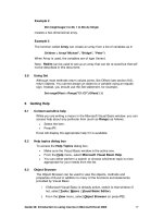
For example, suppose that you want to borrow $10,000 over 5 years with no balloon pay-
ment and a monthly payout of $200. What rate will satisfy these criteria? The worksheet in
Figure 18.9 uses
RATE() to derive the result of 7.4%. Here are some notes about this
model:
■ The term is in years, so the RATE() function’s nper argument multiplies the term by 12.
■ The payment is already a monthly number, so no adjustment is necessary for the pmt
attribute.
■ The payment is negative because it’s money that you pay to the lender.
■ The result of the RATE() function is multiplied by 12 to get the annual interest rate.
Figure 18.9
This worksheet uses
RATE() to determine

the interest rate required
to pay a $10,000 loan
over 5 years at $200
per month.
Calculating How Much You Can Borrow
If you know the current interest rate that your bank is offering for loans, when you want to
have the loan paid off, and how much you can afford each month for the payments, you
might then wonder what is the maximum amount you can borrow under those terms? To
463
Working with Mortgages
figure this out, you need to solve for the principal—that is, present value. You do that in
Excel by using the
PV() function:
PV(rate, nper, pmt[, fv][, type])
rate
The fixed rate of interest over the term of the loan.
nper The number of payments over the term of the loan.
pmt The periodic payment.
fv The future value of the loan (the default is 0).
type The type of payment. Use 0 (the default) for end-of-
period payments; use
1 for beginning-of-period pay-
ments.
For example, suppose that the current loan rate is 6%, you want the loan paid off in 5
years, and you can afford payments of $500 per month. Figure 18.10 shows a worksheet
that calculates the maximum amount that you can borrow—$25,862.78—using the follow-
ing formula:
=PV(B2 / 12, B3 * 12, B4, B5, B6)
18
Figure 18.10

This worksheet uses
PV() to calculate the
maximum principal that
you can borrow,given a
fixed interest rate,term,
and monthly payment.
Working with Mortgages
For both businesses and people,a mortgage is almost always the largest financial transaction.Whether it’s millions of
dollars for a new building or hundreds of thousands of dollars for a house,a mortgage is serious business.It pays to know
exactly what you’re getting into,both in terms of long-term cash flow and in terms of making good decisions up front
about the type of mortgage so that you minimize your interest costs.This case study takes a look at mortgages from both
points of view.
CASE STUDY
Building a Variable-Rate Mortgage Amortization Schedule
For simplicity’s sake,it’s possible to build a mortgage amortization schedule like the ones shown earlier in this chapter.
However,these are not always realistic because a mortgage rarely uses the same interest rate over the full amortization
period.Instead,you usually have a fixed rate over a specific term (usually 1 to 5 years),and you then renegotiate the
mortgage for a new term.This renegotiation involves changing three things:
■ The interest rate over the coming term,which will reflect current market rates.
■ The amortization period, which will now be shorter by the length of the previous term.For example,a 25-year
amortization will drop to a 20-year amortization after a 5-year term.
■ The present value of the mortgage,which will be the remaining principal at the end of the term.
Figure 18.11 shows an amortization schedule that takes these mortgage realities into account.
18
Chapter 18 Building Loan Formulas
464
Figure 18.11
A mortgage amortization
that reflects the changing
interest rates,amortiza-

tion periods,and present
value at each new term.
Here’s a summary of what’s happening with each column in the amortization:
■ Amortization Year—This column gives the year of the overall amortization.This is mainly used to help calculate
the Term Period values.Note that the values in this column are generated automatically based on the value in the
Amortization (Years) cell (B3).
■ Term Period—This column gives the year of the current term.This is a calculated value (it uses the MOD()
function) based on the value in the Amortization Year column and the value in the Term (Years) cell (B4).
465
Working with Mortgages
18
■ Interest Rate—This is the interest rate applied to each term.You enter these rates by hand.
■ NPER—This is the amortization period applied to each term.It’s used as the nper argument for the PMT(),
PPMT(),and IPMT() functions.You enter these values by hand.
■ Payment—This is the monthly payment for the current term.The PMT() function uses the Interest Rate column
value for the rate argument and the NPER column value for the nper argument.For the pv argument,the func-
tion grabs the remaining balance at the end of the previous term by using the OFFSET() function in the follow-
ing general form:
OFFSET(current_cell, -Term_Period, 5)
Here,current_cell is a reference to the cell containing the formula,and Term_Period is a reference to the
corresponding cell in the Term Period column.For example,here’s the formula in E11:
OFFSET(E11, -B11, 5)
Because the value in B11 is 1,the function goes up one row and right five columns,which returns the value in J10
(in this case,the original principal).
■ Principal and Interest—These columns calculate the principal and interest components of the payment,and
they use the same techniques as the Payment column does.
■ Cumulative Principal and Cumulative Interest—These columns calculate the total principal and interest paid
through the end of each year. Because the interest rate isn’t constant over the life of the loan,you can’t use
CUMPRINC() and CUMIPMT().Instead,these columns use running SUM() functions.
■ Remaining Principal—This column calculates the principal left on the loan by subtracting the value in the

Principal column for each year. At the end of each term,the Remaining Principal value is used as the pv argument
in the PMT(),PPMT(),and IPMT() functions over the next term.In Figure 18.11,for example,at the end of the
first 5-year term,the remaining principal is $89,725.43,so that’s the present value used throughout the second
5-year term.
Allowing for Mortgage Principal Paydowns
Many mortgages today allow you to include in each payment an extra amount that goes directly to paying down the
mortgage principal.Before you decide to take on the financial burden of these extra paydowns,you probably want two
questions answered:
■ How much quicker will I pay off the mortgage?
■ How much money will I save over the amortization period?
Both questions are easily answered using Excel’s financial functions. Consider the mortgage-analysis model I’ve set up in
Figure 18.12.The Initial Mortgage Data area shows the basic numbers needed for the calculations:the annual interest
rate (cell B2),the amortization period (B3), the principal (B4),and the paydown that is to be added to each payment
(B5—notice that this is a negative number because it represents a monetary outflow).
The Payment Adjustments area contains four values:
■ Payment Frequency—Use this drop-down list to specify how often you make your mortgage payments.The
available values—Annual,Monthly, Semimonthly, Biweekly,and Weekly—come from the range D8:D12;the
number of the selected list item is stored in cell C8.
■ Payments Per Year (D3)—This is the number of payments per year, as given by the following formula:
=CHOOSE(E2, 1, 12, 24, 26, 52)
■ Rate Per Payment—This is the annual rate divided by the number of payments per year.
■ Total Payments—This is the amortization value multiplied by the number of payments per year.
The Mortgage Analysis area shows the results of various calculations:
■ Frequency Payment (Frequency is the selected item in the drop-down list.)—The Regular Mortgage payment
(B15) is calculated using the PMT() function, where the rate argument is the Rate Per Payment value (D10) and
the nper argument is the Total Payments value (B11):
=PMT(E4, E5, B4, 0, 0)
The With Extra Payment value (C15) is the sum of the Paydown (B5) and the Regular Mortgage payment (B15).
■ Total Payments—For the Regular Mortgage (B16),this is the same as the Total Payments value (B11).It’s copied
here to make it easy for you to compare this value with the With Extra Payment value (C16),which calculates the

revised term with the extra paydown included.It does this with the NPER() function,where the rate argument
is the Rate Per Payment value (B10) and the pmt argument is the payment in the With Extra Payment column
(C15).
18
Chapter 18 Building Loan Formulas
466
Figure 18.12
A mortgage-analysis
worksheet that calculates
the effect of making
extra monthly paydowns
toward the principal.
467
Working with Mortgages
■ Total Paid—These values multiply the Payment value by the Total Payments value for each column.
■ Savings—This value (cell C18) takes the difference between the Total Paid values,to show how much money you
save by including the paydown in each payment.
In the example shown in Figure 18.12,paying an extra $100 per month toward the mortgage principal reduces the term
on a $100,000 mortgage from 300 months (25 years) to 223.4 months (about 18 1/2 years),and reduces the total
amount paid from $193,290 to $166,251,a savings of $27,039.
18
From Here
■ To learn how to add a list box to a worksheet, see “Using Dialog Box Controls on a
Worksheet,” p. 105.
■ The RATE() function uses iteration to calculate its value. To learn more about iteration,
see “Using Iteration and Circular References,” p. 95.
■ Many of the functions you learned in this chapter—including PMT(), RATE(), and
NPER()—can also be used with investment calculations. See “Building Investment
Formulas,” p. 469.
■ The PV() function is most often used in discount calculations. See “Calculating the

Present Value,” p. 484.
This page intentionally left blank
IN THIS CHAPTER
Building Investment
Formulas
19
The time value of money concepts introduced in
Chapter 18, “Building Loan Formulas,” apply
equally well to investments. The only difference is
that you need to reverse the signs of the cash val-
ues. That’s because loans generally involve receiving
a principal amount (positive cash flow) and paying
it back over time (negative cash flow). An invest-
ment, on the other hand, involves depositing
money into the investment (negative cash flow) and
then receiving interest payments (or whatever) in
return (positive cash flow).
With this sign change in mind, this chapter takes
you through some Excel tools for building invest-
ment formulas. You’ll learn about the wonders of
compound interest; how to convert between nomi-
nal and effective interest rates; how to calculate the
future value of an investment; ways to work toward
an investment goal by calculating the required
interest rate, term, and deposits; and how to build
an investment schedule.
Working with Interest Rates
As I mentioned in Chapter 18, the interest rate is
the mechanism that transforms a present value into
a future value. (Or, operating as a discount rate, it’s

what transforms a future value into a present value.)
Therefore, when working with financial formulas,
it’s important to know how to work with interest
rates and to be comfortable with certain terminol-
ogy. You’ve already seen (again, in Chapter 18) that
it’s crucial for the interest rate, term, and payment
to use the same time basis. The next sections show
you a few other interest rate techniques you should
know.
Working with Interest Rates . . . . . . . . . . . . .469
Calculating the Future Value . . . . . . . . . . . . .472
Working Toward an Investment Goal . . . . . .474
Building an Investment Schedule . . . . . . . . .479
Understanding Compound Interest
An interest rate is described as simple if it pays the same amount each period. For example,
if you have $1,000 in an investment that pays a simple interest rate of 10% per year, you’ll
receive $100 each year.
Suppose, however, that you were able to add the interest payments to the investment.
At the end of the first year, you would have $1,100 in the account, which means that you
would earn $110 in interest (10% of $1,100) the second year. Being able to add interest
earned to an investment is called compounding, and the total interest earned (the normal
interest plus the extra interest on the reinvested interest—the extra $10, in the example)
is called compound interest.
Nominal Versus Effective Interest
Interest can also be compounded within the year. For example, suppose that your $1,000
investment earns 10% compounded semiannually. At the end of the first 6 months, you
receive $50 in interest (5% of the original investment). This $50 is reinvested, and for the
second half of the year, you earn 5% of $1,050, or $52.50. Therefore, the total interest
earned in the first year is $102.50. In other words, the interest rate appears to actually be
10.25%. So which is the correct interest rate, 10% or 10.25%?

To answer that question, you need to know about the two ways that most interest rates are
most often quoted:
■ The nominal rate—This is the annual rate before compounding (the 10% rate, in the
example). The nominal rate is always quoted along with the compounding frequency—
for example, 10% compounded semiannually.
19
Chapter 19 Building Investment Formulas
470
The nominal annual interest rate is often shortened to APR,or the annual percentage rate.
NOTE
■ The effective rate—This is the annual rate that an investment actually earns in the
year after the compounding is applied (the 10.25%, in the example).
In other words, both rates are “correct,” except that, with the nominal rate, you also need
to know the compounding frequency.
If you know the nominal rate and the number of compounding periods per year (for exam-
ple, semiannually means two compounding periods per year, and monthly means 12 com-
pounding periods per year), you get the effective rate per period by dividing the nominal
rate by the number of periods:
=nominal_rate / npery
471
Working with Interest Rates
Here, npery is the number of compounding periods per year. To convert the nominal
annual rate into the effective annual rate, you use the following formula:
=((1 + nominal_rate / npery) ^ npery) - 1
Conversely, if you know the effective rate per period, you can derive the nominal rate
by multiplying the effective rate by the number of periods:
=effective_rate * npery
To convert the effective annual rate to the nominal annual rate, you use the following
formula:
npery * (effective_rate + 1) ^ (1 / npery) - npery

Fortunately, the next section shows you two functions that can handle the conversion
between the nominal and effective annual rates for you.
Converting Between the Nominal Rate and the Effective Rate
To convert a nominal annual interest rate to the effective annual rate, use the EFFECT()
function:
EFFECT(nominal_rate, npery)
nominal_rate
The nominal annual interest rate
npery The number of compounding periods in the year
For example, the following formula returns the effective annual interest rate for an
investment with a nominal annual rate of 10% that compounds semiannually:
=EFFECT(0.1, 2)
Figure 19.1 shows a worksheet that applies the EFFECT() function to a 10% nominal annual
rate using various compounding frequencies.
19
Figure 19.1
The formulas in column D
use the
EFFECT()
function to convert the
nominal rates in column
C to effective rates based
on the compounding
periods in column B.
19
Chapter 19 Building Investment Formulas
472
If you already know the effective annual interest rate and the number of compounding peri-
ods, you can convert the rate to the nominal annual interest rate by using the
NOMINAL()

function:
NOMINAL(effect_rate, npery)
effect_rate
The effective annual interest rate
npery The number of compounding periods in the year
For example, the following formula returns the nominal annual interest rate for an invest-
ment with an effective annual rate of 10.52% that compounds daily:
=NOMINAL(0.1052, 365)
Calculating the Future Value
Just as the payment is usually the most important value for a loan calculation, the future
value is usually the most important value for an investment calculation. After all, the pur-
pose of an investment is to place a sum of money (the present value) in some instrument for
a time, after which you end up with some new (and hopefully greater) amount: the future
value.
To calculate the future value of an investment, Excel offers the
FV() function:
FV(rate, nper[, pmt][, pv][, type])
rate
The fixed rate of interest over the term of the
investment.
nper The number of periods in the term of the
investment.
pmt The amount deposited in the investment each
period (the default is
0).
pv The initial deposit (the default is 0).
type The type of deposit. Use 0 (the default) for end-of-
period deposits; use
1 for beginning-of-period
deposits.

Because both the amount deposited per period (the
pmt argument) and the initial deposit
(the
pv argument) are sums that you pay out, these must be entered as negative values in
the
FV() function.
You can download the workbook that contains this chapter’s examples here:
www.mcfedries.com/Excel2007Formulas/
NOTE
473
Calculating the Future Value
The next few sections take you through various investment scenarios using the FV()
function.
The Future Value of a Lump Sum
In the simplest future value scenario, you invest a lump sum and let it grow according to
the specified interest rate and term, without adding any deposits along the way. In this case,
you use the
FV() function with the pmt argument set to 0:
FV(rate, nper, 0, pv, type)
For example, Figure 19.2 shows the future value of $10,000 invested at 5% over 10 years.
19
Figure 19.2
When calculating the
future value of an initial
lump sum deposit,set the
FV() function’s pmt
argument to 0.
The Future Value of a Series of Deposits
Another common investment scenario is to make a series of deposits over the term of the
investment, without depositing an initial sum. In this case, you use the

FV() function with
the
pv argument set to 0:
FV(rate, nper, pmt, 0, type)
For example, Figure 19.3 shows the future value of $100 invested each month at 5% over
10 years. Notice that the interest rate and term are both converted to monthly amounts
because the deposit occurs monthly.
Excel’s FV() function doesn’t work with continuous compounding.Instead, you need to use a
worksheet formula that takes the following general form:
=pv * e ^ (rate * nper)
For example,the follow formula calculates the future value of $10,000 invested at 5% over 10
years compounded continuously (and returns a value of $16,487.21):
=10000 * EXP(0.05 * 10)
TIP
19
Chapter 19 Building Investment Formulas
474
The Future Value of a Lump Sum Plus Deposits
For best investment results, you should invest an initial amount and then add to it with reg-
ular deposits. In this scenario, you need to specify all the
FV() function arguments (except
type). For example, Figure 19.4 shows the future value of an investment with a $10,000 ini-
tial deposit and $100 monthly deposits at 5% over 10 years.
Figure 19.3
When calculating the
future value of a series of
deposits,set the
FV()
function’s pv argument
to

0.
Figure 19.4
This worksheet uses the
full
FV() function syn-
tax to calculate the future
value of a lump sum plus
a series of deposits.
Working Toward an Investment Goal
Instead of just seeing where an investment will end up, it’s often desirable to have a specific
monetary goal in mind and then ask yourself, “What will it take to get me there?”
Answering that question means solving for one of the four main future value parameters—
interest rate, number of periods, regular deposit, and initial deposit—while holding the
other parameters (and, of course, your future value goal) constant. The next four sections
take you through this process.
Calculating the Required Interest Rate
If you know the future value that you want, when you want it, and the initial deposit and
periodic deposits you can afford, what interest rate do you require to meet your goal? You
475
Working Toward an Investment Goal
answer that question using the RATE() function, which you first encountered in Chapter 18.
Here’s the syntax for that function from the point of view of an investment:
➔ To work with the RATE() function in a loan context,see“Calculating the Interest Rate Required for a Loan,”p. 461.
RATE(nper, pmt, pv, fv[, type][, guess])
nper
The number of deposits over the term of the invest-
ment.
pmt The amount invested with each deposit.
pv The initial investment.
fv The future value of the investment.

type The type of deposit. Use 0 (the default) for end-of-
period deposits; use
1 for beginning-of-period
deposits.
guess A percentage value that Excel uses as a starting point
for calculating the interest rate (the default is 10%).
For example, if you need $100,000 ten years from now, are starting with $10,000, and can
deposit $500 per month, what interest rate is required to meet your goal? Figure 19.5
shows a worksheet that comes up with the answer: 6%.
19
Figure 19.5
Use the RATE() func-
tion to work out the
interest rate required to
reach a future value given
a fixed term,a periodic
deposit,and an initial
deposit.
Calculating the Required Number of Periods
Given your investment goal, if you have an initial deposit and an amount that you can
afford to deposit periodically, how long will it take to reach your goal at the prevailing
market interest rate? You answer this question by using the
NPER() function (which was
introduced in Chapter 18). Here’s the
NPER() syntax from the point of view of an
investment:
➔ To work with the NPER() function in a loan context,see“Calculating the Term of the Loan,”p. 459.
19
Chapter 19 Building Investment Formulas
476

NPER(rate, pmt, pv, fv[, type])
rate The fixed rate of interest over the term of the invest-
ment.
pmt The amount invested with each deposit.
pv The initial investment.
fv The future value of the investment.
type The type of deposit. Use 0 (the default) for end-of-
period deposits; use
1 for beginning-of-period
deposits.
For example, suppose that you want to retire with $1,000,000. You have $50,000 to invest,
you can afford to deposit $1,000 per month, and you expect to earn 5% interest. How long
will it take to reach your goal? The worksheet in Figure 19.6 answers this question: 349.4
months, or 29.1 years.
Figure 19.6
Use the NPER()
function to calculate how
long it will take to reach a
future value,given a fixed
interest rate,a periodic
deposit,and an initial
deposit.
Calculating the Required Regular Deposit
Suppose that you want to reach your future value goal by a certain date and that you have
an initial amount to invest. Given current interest rates, how much extra do you have to
deposit into the investment periodically to achieve your goal? The answer here lies in the
PMT() function from Chapter 18. Here are the PMT() function details from the point of view
of an investment:
➔ To work with the PMT() function in a loan context,see“Calculating the Loan Payment,”p. 450.
PMT(rate, nper, pv, fv[, type])

rate
The fixed rate of interest over the term of the
investment.
nper The number of deposits over the term of the
investment.
477
Working Toward an Investment Goal
pv The initial investment.
fv The future value of the investment.
type The type of deposit. Use 0 (the default) for end-of-
period deposits; use
1 for beginning-of-period
deposits.
For example, suppose that you want to end up with $50,000 in 15 years to finance your
child’s college education. If you have no initial deposit and you expect to get 7.5% interest
over the term of the investment, how much do you need to deposit each month to reach
your target? Figure 19.7 shows a worksheet that calculates the result using
PMT(): $151.01
per month.
19
Figure 19.7
Use the PMT() function
to derive how much you
need to deposit periodi-
cally to reach a future
value,given a fixed inter-
est rate,a number of
deposits,and an initial
deposit.
Calculating the Required Initial Deposit

For the final standard future value calculation, suppose that you know when you want to
reach your goal, how much you can deposit each period, and how much the interest rate
will be. What, then, do you need to deposit initially to achieve your future value target? To
find the answer, you use the
PV() function, which uses the following syntax from the point
of view of an investment:
➔ To work with the PV() function in a discount context,see“Calculating the Present Value,”p. 484.
PV(rate, nper, pmt, fv[, type])
rate
The fixed rate of interest over the term of the
investment.
nper The number of deposits over the term of the invest-
ment.
pmt The amount invested with each deposit.
fv The future value of the investment.
type The type of deposit. Use 0 (the default) for end-of-
period deposits; use
1 for beginning-of-period
deposits.
19
Chapter 19 Building Investment Formulas
478
For example, suppose that your goal is to end up with $100,000 in 3 years to purchase new
equipment. If you expect to earn 6% interest and can deposit $2,000 monthly, what does
your initial deposit have to be to make your goal? The worksheet in Figure 19.8 uses
PV()
to calculate the answer: $17,822.46.
Figure 19.8
Use the PV() function
to find out how much you

need to deposit initially
to reach a future value,
given a fixed interest rate,
number of deposits,and
periodic deposit.
Calculating the Future Value with Varying Interest Rates
The future value examples that you’ve worked with so far have all assumed that the interest
rate remained constant over the term of the investment. This will always be true for fixed-
rate investments, but for other investments, such as mutual funds, stocks, and bonds, using
a fixed rate of interest is, at best, a guess about what the average rate will be over the term.
For investments that offer a variable rate over the term, or when the rate fluctuates over
the term, Excel offers the
FVSCHEDULE() function, which returns the future value of some
initial amount, given a schedule of interest rates:
FVSCEDULE(principal, schedule)
principal
The initial investment
schedule A range or array containing the interest rates
For example, the following formula returns the future value of an initial $10,000 deposit
that makes 5%, 6%, and 7% over 3 years:
=FVSCHEDULE(10000, {0.5, 0.6, 0.7})
Similarly, Figure 19.9 shows a worksheet that calculates the future value of an initial
deposit of $100,000 into an investment that earns 5%, 5.5%, 6%, 7%, and 6% over 5
years.
If you want to know the average rate earned on the investment,use the RATE() function, where
nper is the number of values in the interest rate schedule,pmt is 0, pv is the initial deposit,and
fv is the negative of the FVSCHEDULE() result.Here’s the general syntax:
RATE(ROWS(schedule), 0, principle, -FVSCHEDULE(principal,
schedule))
NOTE

Building an Investment Schedule
If you’re planning future cash-flow requirements or future retirement needs,it’s often not enough just to know how
much money you’ll have at the end of an investment.You might need to also know how much money is in the invest-
ment account or fund at each period throughout the life of the investment.
To do this,you need to build an investment schedule.This is similar to an amortization schedule,except that it shows the
future value of an investment at each period in the term of the investment.
➔ To learn about amortization schedules,see“Building a Loan Amortization Schedule,”p. 456.
In a typical investment schedule,you need to take two things into account:
■ The periodic deposits put into the investment,particularly the amount deposited and the frequency of the
deposits.The frequency of the deposits determines the total number of periods in the investment.For example, a
10-year investment with semiannual deposits has 20 periods.
■ The compounding frequency of the investment (annually,semiannually,and so on).Assuming that you know the
APR (that is,nominal annual interest rate),you can use the compounding frequency to determine the effect rate.
Note,however, that you can’t simply use the EFFECT() function to convert the known nominal rate into the effective
rate.That’s because you’re going to calculate the future value at the end of each period,which might or might not corre-
spond to the compounding frequency.(For example,if the investment compounds monthly and you deposit semiannu-
ally,there will be 6 months of compounding to factor into the future value at the end of each period.)
Getting the proper effective rate for each period requires three steps:
1. Use the EFFECT() function to convert the nominal annual rate into the effective annual rate,based on the com-
pounding frequency.
2. Use the NOMINAL() function to convert the effective rate from step 1 into the nominal rate,based on the deposit
frequency.
3. Divide the nominal rate from step 2 by the deposit frequency to get the effective rate per period.This is the value
that you’ll plug into the
FV() function.
479
Building an Investment Schedule
19
Figure 19.9
Use the

FVSCHEDULE()
function to return the
future value of an initial
deposit in an investment
that earns varying rates
of interest.
CASE STUDY
19
Chapter 19 Building Investment Formulas
480
Figure 19.10 shows a worksheet that implements an investment schedule using this technique.
Figure 19.10
An investment schedule
that takes into account
deposit frequency and
compounding frequency
to return the future value
of an investment at the
end of each deposit
period.
Here’s a summary of the items in the Investment Data portion of the worksheet:
■ Nominal Rate (APR) (B2)—This is the nominal annual rate of interest for the investment.
■ Term (Years) (B3)—This is the length of the investment,in years.
■ Initial Deposit (B4)—This is the amount deposited at the start of the investment.Enter this as a negative
number (because it’s money that you’re paying out).
■ Periodic Deposit (B5)—This is the amount deposited at each period of the investment.(Again, this number must
be negative.)
■ Deposit Type (B6)—This is the type argument of the FV() function.
■ Deposit Frequency—Use this drop-down list to specify how often the periodic deposits are made.The available
values—Annually,Semiannually,Quarterly, Monthly,Weekly, and Daily—come from the range F2:F7;the number

of the selected list item is stored in cell E2.
■ Deposits Per Year (D3)—This is the number of periods per year,as given by the following formula:
=CHOOSE(E2, 1, 2, 4, 12, 52, 365)
■ Compounding Frequency—Use this drop-down list to specify how often the investment compounds.You get
the same options as in the Deposit Frequency list.The number of the selected list item is stored in cell E4.
■ Compounds Per Year (D5)—This is the number of compounding periods per year, as given by the
following formula:
=CHOOSE(E4, 1, 2, 4, 12, 52, 365)
481
Building an Investment Schedule
19
■ Effective Rate Per Period (D6)—This is the effective interest rate per period,as calculated using the three-step
algorithm outlined earlier in this section.Here’s the formula:
=NOMINAL(EFFECT(B2, D5), D3) / D3
■ Total Periods (D7)—This is the total number of deposit periods in the loan,which is just the term multiplied by
the number of deposits per year.
Here’s a summary of the columns in the Investment Schedule portion of the worksheet:
■ Period (column A)—This is the period number of the investment.The Period values are generated automatically
based on the Total Periods value (D7).
➔ The dynamic features used in the investment schedule are similar to those used in the dynamic amortization schedule;see“Building a
Dynamic Amortization Schedule,”p. 458.
■ Interest Earned (column B)—This is the interest earned during the period.It’s calculated by multiplying the
future value from the previous period by the Effective Rate Per Period (D6).
■ Cumulative Interest (column C)—This is the total interest earned in the investment at the end of each period.
It’s calculated by using a running sum of the values in the Interest Earned column.
■ Cumulative Deposits (column D)—This is the total amount of the deposits added to the investment at the end
of each period.It’s calculated by multiplying the Periodic Deposit (B5) by the current period number (column A).
■ Total Increase (column E)—This is the total amount by which the investment has increased over the Initial
Deposit at the end of each period.It’s calculated by adding the Cumulative Interest and the Cumulative Deposits.
■ Future Value (column F)—This is the value of the investment at the end of each period.Here’s the FV() formula

for cell A11:
=FV($D$6, A11, $B$5, $B$4, $B$6)
From Here
■ To get the details on the concept of the time value of money, see “Understanding the
Time Value of Money,” p. 449.
■ To work with the RATE() function in a loan context, see “Calculating the Interest Rate
Required for a Loan,” p. 461.
■ To work with the NPER() function in a loan context, see “Calculating the Term of the
Loan,” p. 459.
■ To work with the PMT() function in a loan context, see “Calculating the Loan
Payment,” p. 450.
■ To work with the PV() function in a discount context, see “Calculating the Present
Value,” p. 484.
■ To learn about amortization schedules, see “Building a Loan Amortization Schedule,”
p. 456.
This page intentionally left blank
IN THIS CHAPTER
Building Discount
Formulas
20
In Chapter 19, “Building Investment Formulas,”
you saw that investment calculations largely use the
same time-value-of-money concepts as the loan cal-
culations that you learned about in Chapter 18,
“Building Loan Formulas.” The difference is the
direction of the cash flows. For example, the pre-
sent value of a loan is a positive cash flow because
the money comes to you; the present value of an
investment is a negative cash flow because the
money goes out to the investment.

Discounting also fits into the time-value-of-money
scheme, and you can see its relation to present
value, future value, and interest earned in the
following equations:
Future value = Present value + interest
Present value = Future value – discount
In Chapter 18, you learned about a form of dis-
counting when you determined how much money
you could borrow (the present value) when you
know the current interest rate that your bank offers
for loans, when you want to have the loan paid off,
and how much you can afford each month for the
payments.
➔ See“Calculating How Much You Can Borrow,”p. 462.
Similarly, in Chapter 19, you learned about another
application of discounting when you calculated
what initial deposit was required (the present value)
to reach a future goal, knowing how much you can
deposit each period and how much the interest rate
will be.
➔ See“Calculating the Required Initial Deposit,”p. 477.
This chapter takes a closer look at Excel’s discount-
ing tools, including present value and profitability,
and cash-flow analysis measures such as net present
value and internal rate of return.
Calculating the Present Value . . . . . . . . . . . .484
Discounting Cash Flows . . . . . . . . . . . . . . . . .488
Calculating the Payback Period . . . . . . . . . . .493
Calculating the Internal Rate of Return . . . .496
Publishing a Book . . . . . . . . . . . . . . . . . . . . . .499

Calculating the Present Value
The time-value-of-money concept tells you that a dollar now is not the same as a dollar in
the future. You can’t compare them directly because it’s like comparing apples and oranges.
From a discounting perspective, the present value is important because it turns those future
oranges into present apples. That is, it enables you to make a true comparison by restating
the future value of an asset or investment in today’s terms.
You know from Chapter 19 that calculating a future value relies on compounding. That is,
a dollar today grows by applying interest on interest, like this:
➔ See“Understanding Compound Interest,”p.470
Year 1: $1.00 × (1 + rate)
Year 2: $1.00 × (1 +
rate) × (1 + rate)
Year 3: $1.00 × (1 +
rate) × (1 + rate) × (1 + rate)
More generally, given an interest
rate and a period nper, the future value of a dollar today
is calculated as follows:
=$1.00 * (1 + rate) ^ nper
Calculating the present value uses the reverse process. That is, given some discount rate, a
future dollar is expressed in today’s dollars by dividing instead of multiplying:
Year 1: $1.00 · (1 +
rate)
Year 2: $1.00 · (1 +
rate) · (1 + rate)
Year 3: $1.00 · (1 +
rate) · (1 + rate) · (1 + rate)
In general, given a discount
rate and a period nper, the present value of a future dollar is
calculated as follows:
=$1.00 / (1 + rate) ^ nper

The result of this formula is called the discount factor, and multiplying it by any future value
restates that value in today’s dollars.
Taking Inflation into Account
The future value tells you how much money you’ll end up with, but it doesn’t tell you how
much that money is worth. In other words, if an object costs $10,000 now and your invest-
ment’s future value is $10,000, it’s unlikely that you’ll be able to use that future value to
purchase the object because it will probably have gone up in price. That is, inflation erodes
the purchasing power of any future value; to know what a future value is worth, you need
to express it in today’s dollars.
For example, suppose that you put $10,000 initially and $100 per month into an investment
that pays 5% annual interest. After 10 years, the future value of that investment will be
$31,998.32. Assuming that the inflation rate stays constant at 2% per year, what is the
investment’s future value worth in today’s dollars?
20
Chapter 20 Building Discount Formulas
484
485
Calculating the Present Value
Here, the discount rate is the inflation rate, so the discount factor is calculated as follows:
=1 / (1.02) ^ 10
This returns 0.82. Multiplying the future value by this discount factor gives the present
value: $26,249.77.
Calculating Present Value Using PV()
You’re probably wondering what happened to Excel’s PV() function. I’ve held off introduc-
ing it so that you could see how to calculate present value from first principles. Now that
you know what’s going on behind the scenes, you can make your life easier by calculating
present values directly using the
PV() function:
PV(rate, nper, pmt[, fv][, type])
rate

The fixed rate over the term of the asset or invest-
ment.
nper The number of periods in the term of the asset or
investment.
pmt The amount earned by the asset or deposited into
the investment with each deposit.
fv The future value of the asset or investment.
type When the pmt occurs. Use 0 (the default) for the end
of each period; use
1 for the beginning of each
period.
For example, to calculate the effect of inflation on a future value, you apply the
PV() func-
tion to the future value, where the
rate argument is the inflation rate:
PV(inflation rate, nper, 0, fv)
20
Any time you set the PV() function’s pmt argument to 0,you can ignore the type argument
because it’s meaningless without any payments.
NOTE
Figure 20.1 shows a worksheet that uses PV() to derive the answer of $26,249.77 using the
following formula:
=PV(B9, B3, 0, -B7)
Note that this is the same result that you derived using the discount factor, which is shown
in Figure 20.1 in cell B10. (The table in D2:E13 shows the various discount factors for
each year.)
The next few sections take you through some examples of using PV() in discounting
scenarios.
Income Investing Versus Purchasing a Rental Property
If you have some cash to invest, one common scenario is to wonder whether the cash is

better invested in a straight income-producing security (such as a bond or certificate) or in
a rental property.
One way to analyze this is to gather the following data:
■ On the fixed-income security side, find your best deal in the time frame you’re looking
at. For example, you might find that you can get a bond that matures in 10 years with a
5% yield.
■ On the rental property side, find out what the property produces in annual rental
income. Also, estimate what the rental property will be worth at the same future date
that the fixed-income security matures. For example, you might be looking at a rental
property that generates $24,000 a year and is estimated to be worth $1 million in 10
years.
Given this data (and ignoring complicating factors such as rental property expenses), you
want to know the maximum that you should pay for the property to realize a better yield
than with the fixed-income security.
To solve this problem, use the
PV() function as follows:
=PV(fixed income yield, nper, rental income, future property value)
Figure 20.2 shows a worksheet model that uses this formula. The result of the PV() func-
tion is $799,235. You interpret this to mean that if you pay less than that amount for the
property, the property is a better deal than the fixed-income security; if you pay more,
you’re better off going the fixed-income route.
20
Chapter 20 Building Discount Formulas
486
Figure 20.1
Using the PV() function
to calculate the effects of
inflation on a future
value.