modeling structured finance cash flows with microsoft excel a step by step guide phần 5 pot
Bạn đang xem bản rút gọn của tài liệu. Xem và tải ngay bản đầy đủ của tài liệu tại đây (806.42 KB, 22 trang )
Delinquency, Default, and Loss Analysis
69
ANALYZING HISTORICAL LOSS CURVES
Vintage loss curves created using a static methodology have two important char-
acteristics that should be identified: severity and timing. The severity is the final
cumulative loss percent per vintage. This is how much of the original balance of a
particular vintage is assumed to be defaulted and uncollectible. The timing is how
much loss has been taken by a certain point in time, ending at the final maturity
of the assets. If the assets in the Model Builder example had final maturities of 24
months, then the timing of loss for any period can be determined by dividing the
cumulative loss percentage in that period by the final cumulative loss percentage
(period 24).
Loss timing is important to understand because it can have profound effects
on structured transactions. If the loss timing is front loaded, which means that
losses take place quickly the assets will erode quickly. This directly impacts excess
spread in a transaction, which is the first source of protection against loss. A
transaction modeled with a front-loaded curve versus a regular curve will require
more enhancement since there is less time for excess spread to generate. Back-loaded
curves, where losses take place near the end of the tenor of the assets also have
special effects on structured transactions. If loss does not take place until late
in the transaction, enhancement needs to be sized and kept for those periods.
If a transaction was modeled with a regular loss curve and losses were actually
back-loaded, important structural features such as triggers and reserve accounts
might be inadequate to protect against the back-loaded loss.
MODEL BUILDER 4.2 CONTINUED
1. Label cell AC38 Weighted Avg Curve. To get a summary of the severity of the
historical loss curves a weighted average curve needs to be created. This is done
using the following formula starting in AC39:
=SUMPRODUCT(C39:OFFSET(B39,0,A39),$C$38:
OFFSET($B$38,0,A39))/SUM($C$38:OFFSET($B$38,0,A39))
Copy this formula down to AC62. Also, since these are the monthly losses, sum
them up in AC64 to get the weighted average loss.
2. Timing should be analyzed on a monthly basis first and then cumulative. Take
the first period’s monthly loss amount and divide it by the sum of all the monthly
loss. Label cell AD38 Timing, and start the following formula in AD39:
=AC39/$AC$64
Copy this formula down to AD62. A sum of this column in AD64 should equal
100 percent.
70 MODELING STRUCTURED FINANCE CASH FLOWS WITH MICROSOFT EXCEL
3. A useful way to observe the timing is to make a cumulative timing curve. Do
this by entering the following formula in AE40:
=AE39+AD40
Notice that this started one more row down than the other formulas to avoid
having the label added in a formula. Copy this formula down to AE62. Model
Builder 4.2 will finish up after the next section on projecting loss curves.
PROJECTING LOSS CURVES
If no trend is evident and there are years of data that encompass the tenor of the
asset, then the weighted average curve created in the previous section can be used
as a projected loss curve. However, most of the time industries and companies go
through cycles of increasing and decreasing loss. Also, particularly with assets in
emerging markets, a relatively short time span of data is available. Both of these
issues create the need to project out loss curves.
The first issue, trending, is observed by looking at the same period for each
vintage. In Model Builder 4.2, the monthly losses have a noticeable decreasing trend.
Look at period 5 in Figure 4.9 and notice that in general each successive vintage after
January 2004 has a decreasing loss amount. Most of the periods are experiencing
such a trend. The company could argue that a weighted average curve based solely
on the data overstates loss because the newer vintages are expected to have a lower
loss amount in later periods, but these amounts are not reported and therefore not
captured in the weighted average loss curve.
A thorough loss analysis when trending is involved requires the ability to
observe the full spectrum of loss an asset may experience from origination to
maturity. Taking the weighted average losses for each period will only produce
accurate curves depending on the breadth of the historical loss data vis-
`
a-vis the
age of the assets. The usefulness of the historical loss curves can be assessed by
determining how many of the loss curves have tracked data from origination to
maturity. As an example, assume the current date is January 2006 and in our
examples the data is provided as early as January 2004. Also assume that the final
maturity of the assets is 24 periods. This means that if originations and loss data is
FIGURE 4.9 Trends should be looked for in vintages across periods.
Delinquency, Default, and Loss Analysis
71
provided monthly, there could be one vintage that has reached maturity or ‘‘termed
out.’’ For instance, loans originated in January 2004, with a final maturity of 24
months should have all matured by January 2006. Since the loss data is from January
2004 through January 2006, there is loss history from every part of the loans’ term.
However, loans originated in April 2004 will only have a partial loss history, since
there would only be 21 months of data (May 2004 to January 2006).
If there is a trend in the data and there are few vintages that have ‘‘termed
out,’’ the earlier vintages will have a strong impact on the weighted average curve.
To account for such trends, the newer vintages need to be adjusted. For instance, if
losses are trending upwards and the later vintages aren’t ‘‘grossed up’’ for expected
loss, the weighted average method will understate loss. The opposite will occur if
losses are trending downwards, resulting in an overstatement of loss.
To account for trends, later vintages need to be adjusted using a timing curve
extrapolated from a set of ‘‘base’’ originations. A ‘‘base’’ origination should be a
historical origination from the static loss data that is demonstrative of the expected
timing of the assets. As long as the asset performance is not extremely volatile, it
would be logical to assume that future assets will take losses in a similar manner.
Third-party timing curves, such as those produced by the Public Securities Associa-
tion (PSA) or rating agencies can be used to adjust losses. Also, more sophisticated
statistical analyses can be performed on the loss data to determine trends. The results
of such analyses would provide a basis for trending. The continuation of Model
Builder 4.2 takes the most fundamental approach to projecting loss.
MODEL BUILDER 4.2 CONTINUED
1. The final step in a complete static loss analysis is adjusting newer vintages to
account for trending. To do this, the monthly loss for each vintage that is not
complete needs to be extrapolated based on timing. First, make room to work
underneath the monthly loss percentage area. Insert enough rows so rows 64
through 67 are clear.
2. Label row 64 in B64 as Loss Sev. Taken. This is how much loss as a percent
of original balance has been taken for each vintage. To get the correct amount
a SUM formula with the OFFSET function needs to be used. For the OFFSET
to reference the correct amount of information per vintage create a row of
descending values starting with 24 in C36, 23 in D36, and so on. Descend the
values until Z36 where the value should be 1. In C64 enter the following formula:
=SUM(C39:OFFSET(C38,C36,0))
This formula will only sum the severities that are derived from historical data.
The importance of the OFFSET becomes clearer later as projected severities are
created in the area.
72 MODELING STRUCTURED FINANCE CASH FLOWS WITH MICROSOFT EXCEL
3. In the next row down, label cell B65 Loss % Taken. This row is a percentage
calculation of how much loss the vintage under analysis has taken compared to
the weighted average timing curve. For instance, the January 2004 vintage has
a full 24 months reported, so it has taken 100 percent of loss that it is expected.
The February 2004 vintage is only 23 months so it is short one month of loss
and has taken slightly less than 100 percent loss. To calculate the percentage of
loss that has been taken, enter the following formula starting in C65:
=OFFSET($AE$38,C36,0)
This formula is a basic OFFSET for the timing curve, depending on the seasoning
of the vintage. Copy this formula through to Z65.
4. By knowing the percentage of loss that has been taken, the calculation for the
percentage of loss that needs to be distributed is determined by subtracting the
prior value by one. Label cell B66 Loss to be Dist. Enter the following formula
in cell C66 and copy it across to Z66:
=1−C65
5. The expected loss is the loss severity taken divided by the loss percent taken
so far. If a vintage has taken 100 percent of its loss, then it will be the same
loss severity, however for vintages that have taken less than 100 percent the
severity will be grossed up. Label cell B67 Expected Loss and enter the following
formula in C67 and copy it across to Z67:
=C64/C65
6. With the expected loss for each vintage calculated, the next step is to project the
monthly loss for periods in the future. This can be done directly in the monthly
loss formula since there is already an IF statement set up. Click on cell C39 and
recall that an IF statement was set so that if there was no data (that is ‘‘’’), then
no data should be populated. However, it is now known that if there is no data,
there should be a projection. The projection is going to be the expected loss
amount multiplied by the projected timing of loss. This is summarized by the
following formula that cell C39 should be updated to:
=IF(C8="",C$67*$AD39,C8/C$38)
This formula reads: If there is no monthly loss data project it by taking a
projected timing curve and multiplying that curve by the expected loss amount,
otherwise the loss is based on historical data. Copy this formula across the range
C39:W62. Only this range should be used since October 2005 onwards has so
few data points that the calculations will cause #DIV/0 errors. At this point the
bottom part of the monthly loss table should look like Figure 4.10.
Delinquency, Default, and Loss Analysis
73
FIGURE 4.10 The additional rows are used to project expected loss.
7. The last step is to create a new weighted average curve, taking into account
the projected amounts. Label cell AG38 Adj. WA Curve andinAG39enterthe
following formula:
=SUMPRODUCT(C39:W39,$C$38:$W$38)/SUM($C$38:$W$38)
Copy this formula down to cell AG62. This is a straightforward weighted
average formula, taking into account ALL of the data for each period (up to
column W). When the individual monthly data is summed in cell AG69, the
difference is apparent between using an adjusted curve and a purely historical
curve when trending is taking place. In the latter example, a loss curve of 9.34
percent would be used, while in the former case a much lower loss curve of 7.01
percent would be used due to trending. See Figure 4.11 for a comparison.
The previous sections described in detail the most common analyses performed
on static loss data, however it is by no means exhaustive. There are many sit-
uations that will require different methodologies such as extremely volatile data,
an insufficient quantity of data, a change in assets, etc. Understanding the fine
detail of each situation and what drives loss is the key to choosing the right
methodology. Two different static loss histories may appear very similar, but the
methodology that should be employed often depends on information that is not
on the data tape. These other methodologies can range from calculation inten-
sive analysis, such as examining the slopes of the worst vintages to a very simple
comparables study.
Regardless of the methodology that is used to analyze loss, understanding loss
and what causes it in a transaction is possibly the most important component of
structured finance modeling. A majority of the structure revolves around the loss
and exists to mitigate it. This will become more apparent as loss expectations are
implemented in the model.
INTEGRATING LOSS PROJECTIONS
The first part of this chapter focuses on understanding loss from a historical
perspective and attempting to extrapolate future loss from the history. This second
part takes the knowledge garnered from the history and applies it so loss can be
74 MODELING STRUCTURED FINANCE CASH FLOWS WITH MICROSOFT EXCEL
FIGURE 4.11 The new adjusted
weighted average curve is less than the
original weighted average curve after
a decreasing loss trend is taken into
account.
taken into account when generating cash flows. Two methods of calculating loss exist
for structured finance modeling: original balance calculation and current balance
calculation. The correct one to use depends on the type of loss curve that is integrated
into the model.
The first method, original balance calculation, multiplies a monthly loss severity
by the original balance of the assets. This is used when historical loss analysis has
been completed on assets and when historical loss severities have been calculated off
of original balance. If 100 percent of the timing curve is taken and there is no credit
for seasoning, the dollar loss amount as a percentage of the asset original balance
should be exactly the same as the gross cumulative loss assumption.
The other method calculates loss by multiplying a monthly default rate (MDR)
by the current balance. Monthly default rates are primarily employed when using
a Standard Default Assumption (SDA) curve as the loss projection. In this case the
dollar amount of loss will not be related to a percent of the original balance.
Regardless of the methodology, something to realize about loss projection is that
it is a percentage of the asset balance. This does not seem that unusual when using a
representative line style of amortization. The assets have been aggregated and should
Delinquency, Default, and Loss Analysis
75
therefore have percentages of loss taken out. However, it may seem unusual when
using a loan level style of amortization because a percentage of loss is taken out of
an individual loan. In reality a loan will either default or not. There is no concept
of part of a loan defaulting. In modeling, however, a loss curve will be applied to
each loan and the results aggregated. This concept becomes more important when
thinking about seasoning and default timing.
The Effects of Seasoning and Default Timing
When a loan has begun to amortize or is seasoned, the expected loss amount will
change because a seasoned loan is on a different part of the loss curve than a new
loan. For example, a loan that is brand new with a final maturity of 24 months
might have a loss curve that is 24 periods in length. By month 24 the loan will have
taken 100 percent of its expected loss. Imagine that the loan was already 10 months
old when it was sold into the transaction. This means that 10 months of loss should
be expected to already have taken place. Figure 4.12 shows the difference of two
loans with different seasoning and their expected remaining loss.
FIGURE 4.12 A new loan will be expected to
take a full 7.01 percent of loss, while a loan
seasoned 10 months is assumed to have already
taken 2.31 percent loss, leaving the expectation
of 4.70 percent of loss to be incurred.
76 MODELING STRUCTURED FINANCE CASH FLOWS WITH MICROSOFT EXCEL
The effects of seasoning are accounted for in a model by calculating the seasoning
of a representative line or individual loan and making sure that the loss applied for
each period corresponds to the correct place on the default curve.
Seasoned loans can also have very different loss expectations depending on the
default timing curve. Earlier, default timing and the problems that can arise from
different default timing curves was discussed. However, all of that analysis assumed
a new loan. If a loan is seasoned and the default timing curve is front loaded, there
is a good chance that the loan has already taken a significant amount of its expected
loss. Once Project Model Builder is complete, the differences in loss expectation due
to seasoning and default timing can be examined by varying the loan age and timing
curve.
MODEL BUILDER 4.3: INTEGRATING DEFAULTS IN ASSET AMORTIZATION
1. Start on the Inputs sheet and label the following cells:
E17: Gross Cumulative Loss
F17: Loss Stress
G17: Loss Timing Curve
H17: SDA Curves
Underneath each label is where the values will be entered. For now enter 1.00%
in cell E18 and name this cell pdrCumLoss1,enter1inF18andnamethecell
pdrLossStress1. Before cells G18 and H18 can be created, some work needs to
be done on the Vectors sheet.
2. On the Vectors sheet Chapter 3 ended on column R. Leave column S blank for
spacing purposes and label cell T4 Defaults. Columns T through X are where the
timing curves will be stored. Label cells T5 through X5 Timing Curve 1, Timing
Curve 2, and so on. Name the range S5:X5 lstDefaultCurve. It is important to
include the blank cell S5 so the data validation list will have the option of a
blank value.
3. While on the Vectors sheet move on to cells Z5:AD5. Label these cells Default
Rate 1, Default Rate 2, and so on. Make sure to leave Y5 and AE5 blank for
spacing purposes. Move on to cell AF5 and label that cell SDA 50%,AG5SDA
100%,andAH5SDA 200 %. Name the range AF5:AI5 lstSDA.
4. Go back to the Inputs sheet and create a data validation list in cell G18 using
lstDefaultCurve as the list range. Name cell G18 pdrLossTime1. Create another
data validation list in H18 using lstSDA.NamecellH18SDA
Loss.
5. At this point there is an input for the loss severity and a selector for timing.
The severity can be entered and changed quickly depending on the historical
loss analysis results. The timing curve has been set up so there are five curves to
choose from. Up to this point only the labeling has been created, so an actual
system of determining timing needs to be implemented. This is best done with a
table that allows time to be parsed in a flexible manner, with the timing of loss
varying between time increments. Since this table takes up room and is different
Delinquency, Default, and Loss Analysis
77
from most of the other items in the model, insert a new sheet after the Cash
Flow sheet and name it Loss Timing. On the Loss Timing sheet, label cell A4
Loss Timing. Label cell A6 Months. Cells D6 through H6 will be the labels for
the loss timing curves. Use a numbering system from 1 to 5, 1 being the number
entered for cell D6, 2 for E6, and so on. At this point, the sheet should look like
Figure 4.13.
6. Still on the Loss Timing sheet enter a 1 in cell A7. This represents the first period
that the loss timing starts with. In cell B7 enter 12. This represents period 12 on
the loss timing curve. What is being created here is the parsing of time that will
be referenced later; in this case period 1 through period 12. A quick method
of making this appear as a label, but retain the number values for referencing
purposes later is to use a custom format for the cell. Right-click cell A7 and
click Format Cells. In the Format Cells dialog box, click the Number tab, select
Custom as the category. In the Type text box enter #,## ‘‘to’’. This should make
the cell look like the cell in Figure 4.14.
The cell will still have a numerical value, but can be read quickly as a parsing
of time. The cells below A7 and B7 should increase according to the interval of
FIGURE 4.13 The loss timing sheet is structured so loss scenarios can be
toggled quickly.
FIGURE 4.14 Using a custom cell format retains the numerical value creating
greater functionality for references later.
78 MODELING STRUCTURED FINANCE CASH FLOWS WITH MICROSOFT EXCEL
time. In this case, cells A8 and B8 will be 13 and 24 respectively. Continue this
pattern down through row 36 so there is a maximum of 360 periods.
7. The purpose of the table made in step 6 is to create possible loss timing scenarios.
Scenario 1 (labeled so in cell D6) will have percentages in cells D8 through D36
that represent the timing of loss during each interval that was set up in the A and
B columns. For example, enter 3.33333333%—or simply enter = 100/30 as an
easier way to get this value—in cell D8. This means that 3.33333333 percent
of the loss severity will be applied to assets in the first year of their term. For
instance, if the loss severity over the life of an asset is expected to be 10 percent,
.33333333 percent (10% * 3.33%) would be expected to occur in the first 12
months. For now assume that 3.33333333 percent of loss will occur in each
interval for Scenario 1 (D8:D36). For 360 periods parsed equally into years this
should equal 100 percent. In fact, a complete timing curve should always equal
100 percent, otherwise an incorrect loss amount is being applied. The other loss
timing scenarios can be left blank for now. Later in the book, when scenario
selection is explained, the other timing scenarios will be entered.
8. Loss timing is often expressed as intervals of time (such as 3.33333333 percent
in months 1 to 12), but models are typically run more granularly such as
monthly, therefore loss timing needs to be converted to the model’s periodicity.
Ultimately a monthly vector will be created so the most logical place to store this
vector is on the Vectors sheet. Remember that in step 2 an area was created for
five Timing Curves (columns T through X). An OFFSET-MATCH combination
is the formula that will be used to pull the correct periodic loss timing. In cell
T7 on the Vectors sheet, enter the following formula:
=OFFSET('Loss Timing'!D$6,MATCH($A7,'Loss Timing'!$A$7:
$A$36,1),0)/12*PmtFreqAdd
This formula is similar to the others that use OFFSET-MATCH, with a few
exceptions. In this case the start of each loss timing scenario is referenced by
column (D$6). That reference cell is offset by matching the current period on the
Vector sheet against the intervals in column A on the Loss Timing sheet only.
The fact that column A is only used is extremely important for this formula
to work correctly. The reason this column is only used is because the type of
MATCH that is being used is set to a 1. This means that the formula will find
the largest value that is less than or equal to the look up value. If the rate for
period 14 were trying to be determined, the largest value on the Loss Timing
sheet’s cells A7:A36 is 13. This corresponds to the second interval of timing on
the Loss Timing sheet, which is the correct interval to be referenced (13 to 24).
A 1 match type works only in the case of referencing the lower bound of the
intervals.
The other exceptions are the divisors in the formula. The amount returned
from the OFFSET-MATCH is based on the interval. To get to the periodic
amount the interval amount needs to be divided by the model’s periodicity. If
Delinquency, Default, and Loss Analysis
79
FIGURE 4.15 The timing curve is represented on
a monthly basis on the Vectors sheet.
the model was always monthly then all that needs to be done is to divide by 12.
However, to automate the model in case the periodicity is quarterly, semiannual,
or annual multiplying by the Payment Frequency Additive is necessary. Make
sure to copy the completed formula through T366. So far this area should look
like Figure 4.15.
9. Still on the Vectors sheet, the next step is to come up with the correct periodic
default rate. This is the final rate that will be applied to a balance to come up
with a dollar amount of loss. This rate consists of severity multiplied against
periodic timing. Also, this area is where any stress should be applied to the loss
curve. Recall that in Step 3 columns Z:AD on the Vector sheet were set aside
for this purpose. In Z7 enter the following formula:
=(pdrCumLoss1*pdrLossStress1)*T7
The formula takes the overall loss severity from the Inputs sheet (pdrCumLoss1),
multiplies it by a stress factor if desired (pdrLossStress1), and then multiplies
that product by the current period’s timing. This formula will produce the rate
that should be applied against the dollar balance to derive the dollar loss amount
for a period. Copy this formula into the range Z7:AD366.
10. So far this section has focused on user-generated loss curves; however, there
are times when a preexisting loss curve should be used, particularly with
long-term assets such as mortgages. Earlier an area was set aside for Standard
Default Assumption (SDA) curves. These curves are fixed amounts that have
been determined by the Public Securities Association (PSA) using decades of
historical data from the U.S. mortgage market. They serve as excellent proxies
to determine loss for mortgage products and occasionally other long term assets.
The most basic SDA curve is 100 percent SDA, which assumes an increase
of .02 percent annual default in the first 29 months (starting with .02 percent),
80 MODELING STRUCTURED FINANCE CASH FLOWS WITH MICROSOFT EXCEL
FIGURE 4.16 100 percent SDA displayed as a line graph.
a level .60 percent annual default for months 30 to 60, and then a decrease
of .0095 percent annual default for months 61 to 120, and finally a level .03
percent for months 121 through 360. 100 percent SDA has a very recognizable
shape in the mortgage industry when graphed as in Figure 4.16.
Multiplying or dividing the values of the 100 percent curve creates variations
of the curve. So a 50 percent SDA curve contains half of the values for each
period of the 100 percent curve, while a 200 percent SDA curve contains twice
the values for each period of the 100 percent curve.
It is important to note that the values from these SDA curves are not the
ones used in a monthly model. Remember that SDA uses a monthly default
rate and the curve constructed above is created with annual rates. Use the
following formula to convert from an annual default rate to a monthly default
rate:
Monthly Default Rate = 100
∗
(1−(1−(Annual Default Rate/100))
(1/12)
)
The values for 50 percent, 100 percent, and 200 percent SDA are stored in
the completed model in the Vectors sheet (AF7:AH366). Copy and paste these
values into the same section of the model being created.
11. The next step that starts bringing the assumptions together is on the Cash Flow
sheet. Go to the Cash Flow sheet and recall that columns M and N were created
and labeled for default information. Cell M7 needs to contain the correct default
rate for the asset pool depending on the selections from the Inputs sheet. Since
there are two types of loss curves that can be used, user generated or SDA, the
formula to determine the default rate will need to have a function that selects
the correct curve based on the Inputs sheet.
One method to select the correct curve is to check to see if one of the Input
sheet cells that select the curve is blank. If a user selected no value for one of
the curves, the other curve must be the one being used. To make sure this is
Delinquency, Default, and Loss Analysis
81
possible, blank cells were included in the ranges as part of the data validation
lists. To make this clearer, the beginning of the formula that should be entered
in M7 starts with an IF statement involving one of the curve assumptions on the
Inputs sheet:
=IF(pdrLossTime1="",
The IF statement checks to see if the Timing Curve assumption is blank. If
this is true, then an SDA curve must be in use; however, if it is false then a
user-generated curve must be in use. It is important as a model operator to
always keep one of the values blank, otherwise there can be confusion and
formulas may not work as intended. The completed formula should appear as:
=IF(pdrLossTime1="",OFFSET(Vectors!$AE$6,A7+Age1,
MATCH(SDA
Loss,lstSDA,0)),OFFSET(Vectors!$X$6,A7+Age1,
MATCH(pdrLossTime1,lstDefaultCurve,0)))
OFFSET-MATCH combinations are used to look up the correct default rate
from the Vectors sheet depending on the type of curve and the age-adjusted
period. Copy and paste this cell down to M366.
12. The final cell to complete the default section is the dollar value calculation of the
periodic defaults in N7. This appears to be a simple formula involving default
rate multiplied by balance, but involves a couple of nuances depending on the
type of default rate being used. A user-generated default curve is calculated
against the original balance of each vintage. If such a curve is being used as
the default assumption, then the default rate should be multiplied against the
original balance of the assets. However, the SDA curve was originally calculated
using the current balance to produce a monthly default rate. If an SDA curve is
being used then the default rate should be multiplied against the current balance
of the assets. The necessary toggle between the user-generated and SDA curve
assumption is implemented with an IF statement similar to step 11:
IF(pdrLossTime1="",L7*M7,$L$7*M7)
If an SDA curve is being used then the current balance is multiplied by the
default rate. If a user-generated curve is being used then the original balance
is multiplied by the default rate. In the case of basing defaults against original
balance, there is a chance that the calculated periodic default could be higher
than the current principal balance. Since it is impossible to default more asset
than exists, this needs to be cleaned up using a MIN formula:
=MIN(L7,IF(pdrLossTime1="",L7*M7,$L$7*M7))
Copy and paste this formula over the range N7:N366.
82 MODELING STRUCTURED FINANCE CASH FLOWS WITH MICROSOFT EXCEL
13. Two additional concepts on the Cash Flow sheet can be finished off once
the default amount is known: actual amortization and actual interest. First,
actual amortization is completed in cell R7. The proper amount of principal
is calculated by taking the beginning balance of the assets less the defaulted
amount and multiplying that by a ratio that represents the notional amortization
for the period. Entering the following formula in R7 accomplishes this:
=(L7−N7)*(1−O7/O6)
Notice that the notional amortization ratio is the current period’s amortization
factor divided by the prior period’s. Copy and paste this formula over the range
R7:R366.
14. Finally this section is completed by entering formulas in two columns for the
actual interest calculation. The first formula carriers over the interest rate from
the notional schedule. Enter the following in cell S7 and copy and paste it over
the range S7:S366:
=F7
Next enter the following formula in T7:
=S7*C7*(L7−N7)
This calculates the dollar amount of interest without the defaulted loans. Copy
and paste this formula over the range T7:T366.
With loss calculations complete, it is important to take a step back and
understand how the loss affects the model in general. Defaults are the principal
balance of loans that are assumed to be losses. Since this principal amount is
uncollectible, it should be removed from the asset pool balance, which is done in
the Ending Balance formula in column V of the Cash Flow sheet. It is critical to
realize that the asset pool balance is reduced each period by defaults. The actual
amortization and interest are two concepts that are immediately and most noticeably
affected by defaults. Many other concepts later in this text are affected by loss so its
calculation and application should be well understood.
The importance of analyzing delinquency, default, and loss needs to be reiterated.
Loss is a core determinant of the performance of a transaction and should be
examined carefully. Such analysis is particularly critical for correctly sizing risk-rated
tranches and understanding the risk of owning an asset that has the possibility of
loss. While this chapter is an excellent introduction to these topics, asset specific
characteristics could require additional analysis and unique methodologies.
Prior to moving on to the liability side of the model, there is one more section
related to the assets: recoveries. After a default occurs, there is the possibility that the
repossession and sale of the defaulted asset and the continued pursuance of credit
collections will recover cash. This concept is the focus of Chapter 5.
CHAPTER
5
Recoveries
A
lthough a defaulted asset generates a loss, there is often an opportunity to recover
cash. Repossessing the asset and selling it is the primary method to achieve this
recovery. The cash received from the sale flows into the structured transaction
from which the asset came and is available for liabilities. While this process is
very straightforward, a number of details need to be understood in order to model
recoveries accurately.
The best approach to explain the nuances of recoveries is to first understand
the relevant terminology. In Chapter 4, a gross loss was defined as an asset that is
defaulted and assumed not to pay. Once that asset is repossessed and sold, the cash
recovered can be subtracted from the original loss amount. The gross loss minus
recovery is known as a net loss.
Net loss = Gross loss amount–Recovery amount
Related to net loss are two terms that are often confused: loss severity and
recovery rate. These are actually inverse concepts. The recovery rate is the amount
recovered divided by the gross loss amount. Loss severity is the ratio between net
loss and gross loss amount. For instance, assume that an asset defaulted and created
a $100 loss. If $80 is recovered from the sale of the asset then there is an 80 percent
recovery rate or a 20 percent loss severity.
Recovery rate = Recovery amount/Gross loss amount
Loss severity = Net loss/Gross loss amount
A final term to define is recovery lag. A recovery does not take place immediately
since certain legal proceedings need to occur, the asset physically needs to be
repossessed, and the sale process executed. A recovery can take from a few months
to a number of years before cash is actually realized. The length of time it takes from
the default date to the recovery of actual cash is known as recovery lag.
An excellent method to understand recoveries is to take a loan from default to
recovery and build a timeline of events. For this example, assume that a U.S. auto
loan begins missing payments in May 2005. The loan continued to miss payments
83
84 MODELING STRUCTURED FINANCE CASH FLOWS WITH MICROSOFT EXCEL
and was classified as a default in August 2005. The balance of the loan at that time
was $1,580. At this point, from a transaction point of view, a default has occurred
and a gross loss of $1,580 would be recorded for August 2005. In the same month,
legal action to repossess the asset begins.
For auto loans in the United States, the legal action can proceed relatively
quickly and a judgment can take place within a few months. Assume in this example
that the servicer gets the repossession ruling in two months. Once a repossession
ruling is in hand, the asset has to be physically seized and in the case of vehicles and
equipment, transported to a liquidation or auction site. Depending on the type of
asset, it can take some time to sell the asset and realize the cash. In this example
assume that the asset is seized, auctioned, and sold for $850 in one month. See
Figure 5.1 for a summary of events.
The above example is only partially complete because some costs need to be
deducted. The most significant costs for nearly all assets are liquidation expenses.
Hiring a company to repossess an asset costs money. So does physically moving
the asset to a liquidation or auction location and having the asset liquidated. These
costs can become very significant, particularly if assets are scattered internationally.
Structured transactions often put restrictions on certain locations if the area is
deemed to be difficult or costly to repossess in and liquidate.
Another cost that is not always included in the recovery assumption is the cost of
carry. When a loan is considered defaulted there is an interest cost to the outstanding
loan until the asset is liquidated and cash is received. This is sometimes not reported
and not included in recovery assumptions. For the purposes of this example there
will be no carry cost assumption.
Going back to the example, the cost of liquidation needs to be deducted
from the recovery proceeds. In this case assume that liquidation costs $200. The
net amount recovered is $650. The recovery rate in this case would be 41.13
percent ($650/$1580) otherwise quantifiable as the loss severity at 58.86 percent
($930/$1580).
While industries have developed typical recovery rates and lag times, a historical
study of recoveries should be completed. This would involve aggregating the data that
was mentioned above and coming up with average recovery amounts, liquidation
FIGURE 5.1 A timeline for the recovery process of a typical defaulted auto loan.
Recoveries
85
costs, and lag times. This historical data analysis differs from those in Chapters 3
and 4 because it is more simplified. Recovery data is often difficult for issuers to
accurately put together on a loan level basis. While that methodology would be ideal
and should be used if available, a simpler approach is often sufficient.
MODEL BUILDER 5.1: HISTORICAL RECOVERY ANALYSIS
1. From the CD-ROM open the fileMB5-1 Raw Data from the Ch05 folder on the
CD-ROM. Save this file as Recovery Data.xls. Notice that this data is the loss
information from the previous chapter, with the addition of some incomplete
recovery information below the loss data. See Figure 5.2 for more detail.
2. In this example, the recovery amounts have been given based on origination
year. Look at cell D39. The 18,603 is the amount that has been recovered
for loans originated in 2004. To make a comparison to the loss amounts, the
aggregated loss for each year is necessary. Using the SUM function and starting
in cell C33, sum up the loss for each vintage month.
3. The SUM function adds up the loss for each month, but the loss for each year is
necessary to compare to the yearly recovery information. This can be achieved
using a SUMIF formula. However, first a YEAR formula is necessary. In cell
C34, use the YEAR function on cell C6. The formula should look like:
= YEAR(C6)
Copy and paste this formula over C34:AA34. This will give the year that each
vintage is associated with and allow the SUMIF to be completed.
4. Go to cell C39 and create SUMIF for the total losses depending on the vintage
year. The formula should read as follows:
= SUMIF($C$34:$AA$34,B39,$C$33:$AA$33)
Copy and paste this formula in cell C40 to get the total for 2006.
FIGURE 5.2 In addition to the loss data a section on recovery information is
contained on the sheet.
86 MODELING STRUCTURED FINANCE CASH FLOWS WITH MICROSOFT EXCEL
FIGURE 5.3 The recovery analysis is shown completed.
5. Liquidation proceeds and costs have been provided in the raw data. Typically
this may require data manipulation to aggregate, but for now assume that it
is presented in this format. The next step is to calculate the net proceeds from
liquidation. This is a simple subtraction formula. In cell F39, enter the following
formula:
= D39 − E39
Copy and paste this formula down to cell F40.
6. The next step is to calculate the recovery rate by dividing the net proceeds by the
amount that was considered lost. This is done in cell G39 using the following
formula:
= F39/C39
Copy and paste this formula down to cell G40.
7. The final part of the analysis is to notice the recovery lag. This is provided in
H39 and H40. Typically the lag should be reported by the servicer or can be
calculated by a more granular analysis. Refer to Figure 5.3 for a look at the
completed section.
The takeaway from this analysis is the recovery rate and lag. In this case,
there are only two years of data, so it is questionable to use averages. With
limited data, it is more conservative to take the lowest recorded recovery and
the longest lag. In this example that would be 40.34 percent and five months.
PROJECTING RECOVERIES IN A CASH FLOW MODEL
Since recoveries are not a guaranteed cash flow, they are often looked upon with
skepticism among risk adverse analysts. Even with data some analysts don’t give
credit for recoveries. However, when there is a recovery assumption it is important
to implement the cash flow correctly. This includes achieving the correct timing of
cash flow depending on lag and directing the cash in a manner consistent with the
transaction structure.
Recoveries
87
MODEL BUILDER 5.2: INTEGRATING RECOVERIES INTO
PROJECT MODEL BUILDER
1. Start at the Inputs sheet in cell J17 and label that cell Recovery Rate. Label cell
K17 Recovery Lag. In cell J18 enter 40% as an approximation of the recovery
rate. Name this cell pdrRecovRate1. In cell K18, enter 5 for the recovery lag.
Name this cell pdrRecovLag1.
2. Switch over to the Cash Flow sheet. Earlier Column U was designated as the area
for recoveries. The formula for the recovery amount has to take into account
the recovery rate and the lag. This can be achieved using an IF statement in
conjunction with an OFFSET function. An IF statement is required first to make
sure there is no calculation prior to the first possible recovery period. Cell U7
should start as follows:
= IF(A7 <= pdrRecovLag1,0
Without such a statement, there would be an error in the periods prior to the
lag period when the OFFSET is implemented. With the IF statement in place,
the OFFSET needs to reference the defaulted amount that occurred in the past.
The periods back should be the recovery lag. Once that defaulted amount is
determined, it should then be multiplied by the recovery rate to get the recovery
amount. The following formula does exactly this:
= IF(A7 <= pdrRecovLag1,0,OFFSET(N7,-pdrRecovLag1,0)*pdrRecovRate1)
The OFFSET starts with the current period’s defaulted amount (cell N7) and
goes back in time using the recovery lag. The lag variable has a negative in front
of it so it seeks a reference cell that is back in time, versus forward in time if it
was positive. Finally, the defaulted amount is multiplied by the recovery rate to
get the recovery amount. Copy this cell down the range U7:U366.
Occasionally, the question of seasoned loans brings up a debate in recoveries
when using the above formula. The debate is that by using this formula one
assumes that no loans default prior to the start of the transaction. Some will
argue that loans could have defaulted in the month prior to the transaction
and if they were in the pool their recovery amount would come in earlier
than the IF statement allows. The deciding point on this debate is that most
structured transactions do not include defaulted loans in the pool of assets. This
would mean that all loans going into the pool are current and the IF statement
assumption holds, even with seasoned loans.
3. At this point the recovery section is complete, but to finish the entire Asset
Amortization section one more column on the Cash Flow sheet needs to be
created. Column X is the final column and is where all the cash flow that
is generated each period will be aggregated. Label cell X4 Total Cash Flow
Available for Liabilities. In cell X7 enter the following formula and copy and
paste it over the range X7:X366:
= Q7+R7+T7+U7
88 MODELING STRUCTURED FINANCE CASH FLOWS WITH MICROSOFT EXCEL
Scheduled Principal, Prepaid Principal, Interest, and Recoveries are real cash
flows in each month and are what are available to the waterfall of liabilities. An
important point about recoveries is that they are included as cash flow for the
waterfall, but do not amortize the asset principal. This means that the cash is
similar to interest in that it helps create excess spread.
FINAL POINTS REGARDING RECOVERIES
The reason the recovery analysis is not as detailed as prepayments or defaults is that
recovery values can be very volatile depending on asset type, geographic region, and
general economic environment. More advanced methods exist for assets, such as
market value decline (MVD), which focuses on home values depending on specific
regions or Automotive Lease Guide (ALG) values for estimating lease residual value,
but these are all advanced analyses that are very dependent on highly detailed
research in a specific industry.
Also, structured transactions are traditionally based on cash flow from the assets,
not recoveries from defaults. As competition increases, newer deals have been giving
more and more credit to recovery values, which can be dangerous if not properly
analyzed. These types of deals begin to look like transactions that should be done by
nonperforming loan (NPL) groups. Structured professionals seeking to do such deals
should understand the recovery analyses performed by NPL groups, because they
are often very comprehensive and detailed. In most instances, those analyses include
loan level recovery and specific collateral analysis. For general modeling purposes or
when first starting out, a more basic, conservative approach should be taken.
CHAPTER
6
Liabilities and the
Cash Flow Waterfall
W
ith asset generation complete, this book now turns to the liability side of the
model. While the asset side is fairly standard for a level payment amortization,
the liability section can vary greatly depending on the unique structure of the
transaction. Due to the variability between deals, the liability side needs to be
constructed with as much flexibility as possible. This is achieved by breaking down
the liabilities into individual components that work similarly and can be moved
around quickly.
Before going into the mechanics of how liabilities are paid, it should be
understood what constitutes a liability. For a structured transaction, any cost that
is to be paid from the cash generated by the assets is a liability. Foremost are costs,
which keep the transaction in existence such as trust, servicer, and rating agency fees.
Next is interest and principal due to the parties who funded the assets. This section
can be very complicated depending on the different risk classes of debt known as
tranches. The method in which these tranches are returned principal can also vary
between transactions and as will be seen in the next chapter, within a transaction.
PRIORITY OF PAYMENTS AND THE CASH FLOW WATERFALL
In actual transactions, how the liability structure functions is dictated by the priority
of payments section of a term sheet. This section is often referred to as a waterfall
because the available cash starts at the top and then trickles down through an ordered
series of liabilities. Each section in the written waterfall explains exactly how the
cash should be allocated before moving onto the next section of the waterfall.
Conceptually, the movement of cash through the waterfall transfers well to
two-dimensional spreadsheet-based modeling because time and order can be orga-
nized using rows and columns. The asset side only used rows for time progression,
meaning that a starting balance would begin on row 1 and the next period the
balance would be adjusted for amortization and displayed on row 2. Although asset
interest, prepayments, defaults, and regular amortization do have a logical order,
the vertical column arrangement does not necessarily suggest an organization based
89
90 MODELING STRUCTURED FINANCE CASH FLOWS WITH MICROSOFT EXCEL
FIGURE 6.1 Cash moves through each period from left to right and then down to
the next period.
on time or priority. For the liability side of the model and the cash flow waterfall
that is created on a spreadsheet, the periods still progress by rows; but the items in
columns are arranged by timing. For example, on the Cash Flow sheet starting from
the left after asset amortization, where cash is available, the liabilities are organized
in priority as one progresses through the columns to the right. Each period, the cash
moves from left to right through the waterfall before progressing to the next period
one row below. See Figure 6.1 for more detail.
The Movement of Cash for an Individual Liability
A standard liability has an assumption such as a rate, fixed amount, or a vector of
rates on the Inputs or Vectors sheets. This assumption is then integrated into the
Cash Flow sheet similar to assets. However, the difference is that each liability will
have a certain priority and can either be paid or not paid depending on how much
cash is available. In such a system, the concept of ‘‘What You Have and What You
Need’’ is essential to understand and make clear.
Barring extremely high default scenarios, every period a certain amount of cash
should be available to pay liabilities. The first liability in the priority of payments will
have all of the cash that is available from the assets for payment. Once that liability
is paid, the cash available is appropriately reduced and the next liability can use the
remaining amount for payment. This continues until the waterfall is done and either
all of the cash for the period is used or excess remains and is released or trapped.