beginning microsoft excel 2010 phần 5 pdf

CHAPTER 4 ■ KEEPING UP APPEARANCES—FORMATTING THE WORKSHEET
146

Figure 4–117. Chromatic scales: Color Scales options
By selecting the second option on the first row—called the Red-Yellow-Green Color Scale, and
applying it to our range of grades, I get this (Figure 4–118):

Figure 4–118. Grade values, colored by score group
In this color scheme, Red captures the highest values, Yellow the intermediate ones, and Green the
lowest—all in shadings to reflect fine differences in values.
The final option—Icon Sets—supplies the user with a large assortment of symbols with which to
format the relationship between values, and in a range of ways (Figure 4–119):
CHAPTER 4 ■ KEEPING UP APPEARANCES—FORMATTING THE WORKSHEET
147

Figure 4–119. Icon Set options
Directional Icon Sets symbolize values by their position in a percentile scale via the designated
icons. Thus if I select the first such option and apply it to the grade range, the conditional format looks
like this (Figure 4–120):

Figure 4–120. An arrow icon set in action
Here we see that the highest scores sport an up arrow, the intermediates a flat one, and the lower
scores a down arrow.
Shapes represent values with a trove of shapes. If I apply the second selection in the Shapes first
column on the grade range, I’ll see this (Figure 4–121):
CHAPTER 4 ■ KEEPING UP APPEARANCES—FORMATTING THE WORKSHEET
148

Figure 4–121. Shape of things to come: the same grades, formatted by shape icons
Here the red diamond captures the highest values, the green circles the intermediates, and the
yellow triangles the lowest .

Ratings communicate value relationships through a potpourri of possibilities—stars, bars, pie
charts, etc. Thus if I choose the pie chart option (the second selection, first column), we’ll see (Figure 4–
122):

Figure 4–122. Bite-sized pie charts
You’ll note, by the way, that the various icons don’t portray values in precisely calibrated ways.
Look at the screen shot above, and you’ll see that the 82, 81, 83, and 77 all display a three-quarter-
blackened pie. That’s because by default Excel organizes the data by their percentage distribution. In
the case of the pies above, Excel assigns a clear icon to those data that fall below 20% of the highest
value in the data, the one-quarter-filled pie for data that occupy the 21-40% percents, and so on. But in
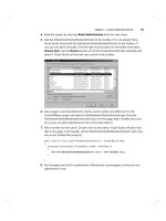
addition to these initial distributions, Excel enables you to customize your own—first by clicking the
Manage Rules…
Continuing with our grade book: If we leave the pie format in place, select these grades in C9:C18,
and click Manage Rules…, we’ll see this (Figure 4–123):
CHAPTER 4 ■ KEEPING UP APPEARANCES—FORMATTING THE WORKSHEET
149

Figure 4–123. Changing the conditional formatting rules
Click Edit Rule… and observe the dialog box shown in Figure 4–124:

Figure 4–124. Rules are made to be…edited
This is a wide-ranging dialog box that contains numerous options, but for now we’re interested in
changing the icon numbers—the score thresholds at which the pies blacken more or less. Note the
defaults about which we’ve already spoken.
Moreover, we see that the Select a Rule Type area in the Edit Formatting Rule dialog box lets you
change your r ule completely; if for example I select Format only values that are above or below average,
I’ll be brought here (Figure 4–125):
CHAPTER 4 ■ KEEPING UP APPEARANCES—FORMATTING THE WORKSHEET
150
`

Figure 4–125. Selecting—and changing—a rule type
And if I click the drop-down arrow by Format values that are (Figure 4–126):

Figure 4–126. Additional rule options
CHAPTER 4 ■ KEEPING UP APPEARANCES—FORMATTING THE WORKSHEET
151
I can select any of these choices, including values that fall within 1, 2, or 3 standard deviations
from the range average. But the larger point is this: by selecting Edit Rule, you can basically replace
your existing Conditional Format with any other sort of rule.
In addition, you can subject the same range to multiple rules. For example, I could compose a
Conditional Format to color blue all the cells with test scores in our range that exceed 80, and to color
red all cells with scores that fall below 60. That is, we could format our range with the Highlight Cells
Rules Greater Than… and Less Than… options. If I went ahead with this plan, my range would take on
this appearance (Figure 4–127):

Figure 4–127. Note some cells meet neither criterion and remain white
And that’s fine. But what if I wanted to color all the cells with scores topping 80 blue, and all the
cells with scores over 85 green? Our wicket has just gotten stickier—because a score such as 90 meets
both conditions. After all, 90 exceeds both 85 and 80—raising the obvious question: which format will I
see in such a cell?
That’s a question Excel wants you to answer—because you’ll need to tell the application which of
the rules will activate first. Once you execute both rules, you’ll want to select the range and click
Manage Rules. Note (Figure 4–128):

Figure 4–128. You need to decide which rule is listed first
The two rules impacting our range are recorded—and in the proper order, because Excel will
simply carry out the rule which appears first in the above dialog box—and we want Excel to consider the
>85 rule before >80, for a simple reason. If >80 is listed first, then even the cell containing 90 will turn
blue—and you’ll never get to >85.
CHAPTER 4 ■ KEEPING UP APPEARANCES—FORMATTING THE WORKSHEET

152
To allow you to arrange your rules in the proper order, you can click on any rule in the Rules
Manager and then click the down arrow button (which the arrow in Figure 4–128 points to).
And if you’ve messed up or simply want to start over, you can purge your worksheet of all your
Conditional Formats, either for particular ranges or the entire sheet, by clicking (Figure 4–129):

Figure 4–129. The Clear Rules option
And choose the appropriate option.
While there’s a large set of permutations crowded into Conditional Formatting, we’ve introduced
the important basics, and you’ll find that with experimentation many of its other features will come to
light.
Just a Bit More…
We can begin to wind down this rather exhaustive—and probably exhausting—résumé of formatting
with a quick look at a curiously-titled button, one holed up in the Cells Group on the Home Tab. It’s
called, as luck would have it… Format, which doesn’t tell you terribly much about what it does. But
when you click its drop-down arrow, it presents a mixed-bag of commands, some of which you wouldn’t
be inclined to call Formatting, and some of which operate on worksheets in their entirety—and we’ll
reserve those for a later chapter. In fact only the upper half of its drop-down menu, shown in Figure 4–
130, concerns us here, listing alternative ways to do some things you already know:
CHAPTER 4 ■ KEEPING UP APPEARANCES—FORMATTING THE WORKSHEET
153

Figure 4–130. Still more formatting options
Clicking Row Height and/or Column Width allows you to modulate the height and/or width of
selected rows and columns (note: unlike the techniques we described earlier, you don’t have to select
row or column headings in order to carry out this option here. If you click in any cell in the row or
column, that will enable you to go ahead with these commands. And you can drag across a range of
rows and columns if you want to change multiple row/column heights and widths. And as you see you
can also execute an Auto Fit of selected columns—but here you will have to select the column headings
before you proceed. Finally, the Default Column Width option doesn’t necessarily do what you think it

will. It doesn’t restore the default width to changed columns; rather it lets you change the default column
width on the worksheet. If you click the command, you’ll see the dialog box shown in Figure 4–131:

Figure 4–131. Establishing a new colunn width
CHAPTER 4 ■ KEEPING UP APPEARANCES—FORMATTING THE WORKSHEET
154
that lets you type a new width, which will apply to all worksheet columns—except those whose widths
you’ve already changed. And don’t ask me why the dialog box is called Standard, and not Default,
Width.
P. S.
And before we bring this chapter to a close, there’s one slightly loose end we need to tie for neatness’
sake. On the chapter’s very first page, I declared that:
“…apart from one obscure exception, formatting data on the worksheet
changes the appearance, and not the value, of those data ”
You’ve politely refrained from asking the big question, so I’ll do it for you: What’s the exception?
It’s this: if you click the File tab, click Options, then click Advanced and scoot down to the When
calculating this workbook section, you’ll take note of an unchecked command call ed Set precision as
displayed. If you check it, any number you’ve formatted with X decimal points will become precisely
that number. That is, if you’ve entered 5.76 in a cell and formatted that value to one decimal point,
you’ll see 5.8. But with Set precision as displayed, 5.8 becomes its value, too—and this is an all-or-
nothing proposition. Turning this option on impacts all the values in the workbook—that is, all its
worksheets. And when you click OK, a prompt on screen reminds of just that: you’ll be told, “Data will
permanently lose accuracy,” meaning your values will take on new, rounded-off values.
And that’s precisely what happens.
IN CONCLUSION…
Long chapter, long subject. That’s because appearances matter. They can’t substitute or cover for
mistaken formulas, or worksheets that don’t deliver the information that’s been requested. You can’t
really fake a spreadsheet, but the ways in which data are presented, or formatted, are integral to the
spreadsheet process too. Think of spreadsheet design as a kind of desktop publishing—and it is—and
the issue becomes clearer. And the next chapter, on charting, picks up the baton and runs with the same

theme. Charts: More than pretty pictures? You bet; just turn the page.
Download From Wow! eBook <www.wowebook.com>
C H A P T E R 5

■ ■ ■

155
The Stuff Of Legend—
Charting in Excel
They say a picture is worth a 1,000 words—a remarkably durable exchange rate to be sure, given how
long they’ve been saying it. But is it true?
As with most such pithy declarations, the answer depends. When it comes to spreadsheets, Excel
jams a toolbox full of charting options for framing some very pretty—and meaningful—pictures of your
data, but wealth needs to be managed wisely.
It makes sense to have the chapter on charts follow our discussion of formatting, because charting
stands right atop the boundary between data manipulation and the way in which that data is presented.
How charts are formatted, and indeed, the very choice of which chart to use, can exert a significant pull
on readers’ perception of what the data mean. It’s one thing to color a number blue, but it can be quite
something else to assign a chart’s vertical axis a minimum value of zero—and if that sounds like Greek to
you, don’t worry, and keep reading.
The point is that, as with formatting in general, Excel’s charting adornments mustn’t get in the way
of the story the chart is attempting to tell. As with comedy, the first rule of charting is: Know your
audience. Think of the charts you see in newspapers and magazines, and ask yourself if they meet your
standard of intelligibility. They probably do, because the chart-makers at these publications understand
the tradeoff between beauty and truth, so to speak, and will likely opt for simplicity over bling. On the
other hand, you may come upon a very different charting environment in a scientific journal, where the
informational needs of readers can be very different.
In any case, Excel makes basic charting almost unnervingly easy, and if you have a few seconds to
spare you’ll have more than enough time to draw a chart up: click in a range of data, click on a chart
type, and—there it is. If you’re happy with the results, you’re done. Yet there’s more to charting than

those quick decisions, or at least there can be; and again, knowing more about how it all works beats
knowing less. So, let's get started.
Starting Charting
First, a bit of terminology. Charts work with data series, which comprise data points. A data series is a
collection of data assigned beneath a category. Thus in this set of data (source: Euromonitor.com)
depicting visitor totals for the top ten tourist cities for 2006 and 2007 (in thousands—that is, the numbers
you see should be multiplied by 1000, shown in Figure 5-1:
CHAPTER 5 ■ THE STUFF OF LEGEND—CHARTING IN EXCEL
156

Figure 5–1. Tourist figures for popular cities—data ripe for charting
both 2006 and 2007 qualify as data series—but if we stand the data on their side, as we shall see, London,
Hong Kong, and all the other city names could serve as series instead (and no, I’ve never been to Antalya,
either). Data points are the individual data items belonging to a series. Thus 15,637.10 is a data point in
the 2006 series.
To actually produce a chart:
1. Click anywhere among the data you want to chart (a point that needs to be
explained),
2. Click the Insert tab, and select from this roster of chart types (Figure 5-2):

Figure 5–2. Chart options
3. Then click any chart type’s down arrow and choose one of the chart variants in
that type, and that’s it, at least for starters. By carrying out the above sequence,
my tourist data could come out looking like this—depending on the chart I
choose, of course (Figure 5-3):
CHAPTER 5 ■ THE STUFF OF LEGEND—CHARTING IN EXCEL
157

Figure 5–3. Those tourist data, brought to a column chart
Estimated time of chart construction: about 4 seconds. Bear in mind that we’re looking at a first pass

at the chart as it would present itself to us by default (note it appears on the same worksheet as the data
that contributed to it), and before we’ve tried our hand at reformatting the result with Excel’s bag of
tricks. Still, 4 seconds is 4 seconds. And a batch of 3-D chart selections is available, too (Figure 5-4):

Figure 5–4. Tourist data in 3-D
CHAPTER 5 ■ THE STUFF OF LEGEND—CHARTING IN EXCEL
158
And charts are dynamic—meaning that any change you make in the source data will automatically
be reflected in the chart. Type a different number in any data cell contributing to the chart, and the
column, or bar, or pie slice tied to that value will experience a change in its size.
Making a Chart of Our Own
But let’s try to construct a chart of our own. In the interests of continuity, we’ll turn back to our test-
grade worksheet, which I’ve entered, sans formatting, in cells C8:I20 (if you have these data on hand
already, you can use those. And you needn’t actually calculate all those averages you see in the data,
though it would be good practice—you can just enter these as numbers here, without writing any
formulas (Figure 5-5):

Figure 5–5. That gradebook
You’ll see there are some important initial points to learn here, so let's look into them.
Excluding Data
As we indicated a few paragraphs above, you could simply click anywhere among the data and
commence the charting process in earnest. But take a look at the screen shot above. Do you want to
chart the scores of a student named Class Averages? Because you will, if you don’t take steps to exclude
that row of data from the chart. And the same question could be asked of the column entitled Average—
do you want its data to be treated as the sixth test in the series of exam results above? Likely not; and so
in order to present Excel with precisely the data we need to in order to complete the chart, we should
select cells C9:H19 (but not the data in the I column—the test averages), as you see in Figure 5-6:
CHAPTER 5 ■ THE STUFF OF LEGEND—CHARTING IN EXCEL
159

Figure 5–6. Selecting gradebook data—averages omitted
Time, then, to modify the chart data selection rule we stated earlier: to start the chart-making
process, you can click anywhere among the data, provided there are no adjoining columns or rows
containing data you don’t want to see in the chart. But in our case, where there are data we want to
exclude, we need to go ahead and select exactly the range we need. And this can be a real-world
scenario.
Once we put these understandings in place and select our range, then all we need do is click one of
the buttons in the Charts group, which identify Excel’s various chart possibilities. Let’s click the Column
button (Figure 5-7):

Figure 5–7. Column chart options
CHAPTER 5 ■ THE STUFF OF LEGEND—CHARTING IN EXCEL
160
Note the array of column chart sub-types. For illustration’s sake, I’ll click the first option on the first
row (titled 2-D Column), yielding this chart (Figure 5-8):

Figure 5–8. Not bad—a first column chart
There’s your chart. Suitable for framing? Probably not, but it does communicate the data pretty
clearly, even if a formatting tweak here and there would help it along. And if you need or want to, you
can delete a chart by clicking on its chart area to select the entire chart, and pressing Delete.
Evaluating the Chart
But before we tweak, let’s review some of the things the chart has done with the data. The chart portrays
each student’s scores for tests 1 through 5, with each test number comprising a data series. The legend—
that column of numbered cubes on the chart’s far right—color-codes each exam series, while the vertical
(value) axis (also known as the Y axis) constructs the scale of values against which each test can be
measured. That scale—here spanning 0 to 120 and subdivided into intervals of 20—is improvised from the
data. Devise a new chart based on a different set of values and the scale could look radically different. The
Horizontal (Category) Axis (also called the X axis) enumerates each student name, placing these beneath
each set of their five scores. It requires a bit of delicacy in view of the thinness of the columns, but if you
position your mouse atop any column in the chart (don’t click) a caption detailing the value of that score

along with the name of the student in question appears (Figure 5-9):
CHAPTER 5 ■ THE STUFF OF LEGEND—CHARTING IN EXCEL
161

Figure 5–9. Captioned information about the data represented by each column
A couple of other definitions need to be introduced here. The Chart Area is the larger background of
the chart, indicated by the arrow at the right of the screen shot above, in Figure 5-9. The Plot Area is the
smaller, rectangular space in which the chart itself is actually positioned, evidenced by the gridlines
above and the left arrow. And you can easily move the chart by clicking the chart arrow, and dragging the
chart wherever you wish on the worksheet. You’ll know you’re in the Chart Area—or any other segment
of the chart, for that matter—by simply resting your mouse over that element and viewing the
identifying caption.
Resizing the Chart
You can also resize the chart by clicking on any one of the chart’s eight resize handles, represented on
the chart’s border by these dots (Figure 5-10):
CHAPTER 5 ■ THE STUFF OF LEGEND—CHARTING IN EXCEL
162

Figure 5–10. Dot’s right—where you can click to resize the chart
Click a handle and drag in the desired direction—left, right, or, on a corner handle, in a diagonal
direction. Dragging diagonally resizes the chart while maintaining the chart’s original aspect ratio, or
the ratio between the chart’s height and width. Dragging a resize handle, left, right, up, or down, on the
other hand, will distort the height-width ratio in one direction or another (Figure 5-11):

Figure 5–11. Sense of proportion—resizing charts is a judgment call
CHAPTER 5 ■ THE STUFF OF LEGEND—CHARTING IN EXCEL
163
These kinds of distortions raise classic questions about the ways in which chart data are presented.
Pinching the chart, as we see above, makes the column bars seem higher than they “really” are.
Flipping the Data Series

Now back to an earlier point about data series. If you click anywhere on the chart, the ribbon takes on
this appearance, showing you the Chart Tools (Figure 5-12):

Figure 5–12. The Chart Tools tab
Each of the Design, Layout, and Format tabs are lined with a set of chart-related button groups.
Click Design, and click the Switch Row/Column button in the Data group, and the chart undergoes this
transformation (Figure 5-13):

Figure 5–13. Same data, different angle
What’s happened? What we’re seeing is a flipping of data series. Whereas our initial chart
designated each of the five tests as a series, here the data have been right-angled, so that the student
names now serve as the series and the tests occupy the Horizontal Axis (tip: the legend will identify the
data series). Our revised chart clusters the student grades by each exam, so that each student is
represented once in each series. In the original chart version, however, the grades are clustered by each
student, so that each exam is represented once in each series. Just keep in mind that the data with which
we’re working in both cases are identical; it’s the data series that have traded places.
This ability to switch and re-designate data series—even as the data used in the switch remain
precisely the same—is an important presentational option, and you need to decide which works for you.
CHAPTER 5 ■ THE STUFF OF LEGEND—CHARTING IN EXCEL
164
Changing The Chart—It’s Your Call
In any case, if you decide the column chart motif isn’t quite what you want, you can readily select a new
chart with by clicking on the chart and then clicking the Change Chart Type in the Type Group, on that
same Design Tab. You’ll trigger this dialog box (Figure 5-14):


Figure 5–14. Change of heart? Change your chart!
The gamut of chart types and sub-types are placed before you for you to select as you see fit—
provided the chart works with your data. And that friendly word of caution serves as a lead-in to a brief
cataloging of the basic chart types, and what they can and can’t do. Some chart usage decisions are

judgment calls, but the fact is that certain sets of data simply can’t be captured by certain kinds of charts,
a point that will become clearer as we proceed.
The Column Chart
Column—perhaps the most commonly deployed chart, and probably the most straightforward. That’s
probably why it’s listed first among the chart types (the order isn’t alphabetical). Column charts,
according to Excel’s own accompanying caption, “are used to compare values across categories.”
Granted, that’s a fairly innocuous description at best, but as we’ve seen, these charts do compare
different categories in an easy-to-understand mode of presentation. Look back at the tourist chart we
composed at the outset of the chapter; both the city and year dimensions are crisply, if not daringly,
portrayed. To mix metaphors, this Clustered Column chart is a garden-variety, vanilla chart, at least until
you jazz it up.
Note, however, that a popular column variant, the Stacked Column, is a touch more subtle, and
Excel offers two kinds of these. The Stacked Column chart piles, or stacks, the values in all chart series
atop one another, for each point on the Horizontal Axis. If that sounds murky, here’s what a Stacked
Column rendering of our grade data looks like (Figure 5-15):
CHAPTER 5 ■ THE STUFF OF LEGEND—CHARTING IN EXCEL
165

Figure 5–15. The Stacked Column chart
Here, and unlike in the standard Clustered Column chart, each student is represented by one
column, which combines all his/her test scores into one aggregate stack. Note the values on the Vertical
axis; they’re far higher than the original, because this chart is adding all the students’ scores.
The 100% Stacked Column is far rarer, and in our illustration treats every student’s total test score
as an individual baseline totaling 100%. Each individual student grade is then stacked to represent the
proportion it contributes to that student’s total (Figure 5-16):

Figure 5–16. A 100% Stacked Column: Where every student scores 100
CHAPTER 5 ■ THE STUFF OF LEGEND—CHARTING IN EXCEL
166
Note the Vertical Axis; every student “scores” 100%, because his/her particular set of scores is

regarded as a whole. We see here that Derek’s low grade of 45 on exam 3 contributes a small green bar to
his total, but all his grades “add up” to 100%. Exotic it is, but the 100% Stacked Chart could be well
applied to a look at the proportions of various types of household expenses contributing to various
families’ budgets.
The Line Chart
The Line chart type is a best seller, too, and is particularly adept at conveying change in a category, e.g., a
ballplayer’s batting averages across his career or a person’s weight across a series of scale
measurements. While in theory this type would be well applied to our test data, there are too many
students in the mix, and thus our line chart presents itself with this tangle (Figure 5-17):

Figure 5–17. Lining up students’ grades: Not a pretty picture
Ready to slap that one on your boss’s desk? Only you can answer that question.
On the other hand, because it features only two data series, the tourist data might be a more suitable
candidate for a Line chart (Figure 5-18):

































CHAPTER 5 ■ THE STUFF OF LEGEND—CHARTING IN EXCEL
167

Figure 5–18. Lining up tourist data
Note here I’ve chosen the Line with Markers chart type, which highlights each data point with a
small symbol.
The Line options also offer Stacked line charts, including a 100% Stacked Line, but these are much
harder to interpret. Here’s our test data in Stacked Line mode (Figure 5-19):

Figure 5–19. How the tests stack up: Test scores via a 100% Stacked Line chart
Here each student’s grades are stacked atop one another in a series of points on the respective lines,
with each line representing each exam. Use with care. You might more profitably apply such a chart to
CHAPTER 5 ■ THE STUFF OF LEGEND—CHARTING IN EXCEL
168

compare, say, the number of home runs hit by the players on different baseball teams, broken out by the
positions they play.
The Pie Chart
The next chart category, Pie, won’t work with our grade data—because pie charts can only capture the
data from one data series at a time. Pie charts treat the data as a single whole, with each data point
contributing one “slice” to the recipe. Thus a purely hypothetical monthly budget that exhibits these
expenses (Figure 5-20):

Figure 5-20. Piece of the pie: One data series—eligible for pie charting
would be eligible for a pie chart, because it consists of merely one series (Figure 5-21):

Figure 5–21. The above data, realized in a pie chart
Now that’s a pretty attractive 4-second chart; but yes, you can add descriptive numbers to the chart
(the actual values or percentages associated with each slice) and other elements, as we’ll see when we
get to chart formatting. (You can’t fashion a pie chart if any of your data points contain a negative
number, by the way; try to imagine how a negative slice could be portrayed.)
Pie charts also offer several “exploded” options; e.g., Figure 5-22:
CHAPTER 5 ■ THE STUFF OF LEGEND—CHARTING IN EXCEL
169

Figure 5–22. Don’t stand too close: An exploded pie chart
Another option enables you to explode just one slice for the sake of emphasizing any one data point
(Figure 5-23):

Figure 5–23. One slice to go
and still another allows you to break out a group of slices on the basis of a criterion you define:
CHAPTER 5 ■ THE STUFF OF LEGEND—CHARTING IN EXCEL
170

Figure 5–24. Selective slicing: identifying pie chart data by a criterion

This customized “explosion” singles out all budget expenses less than $200, for example. (Note: to
select one slice for formatting, click the pie, and then click on the particular slice.)
The Bar Chart
Bar charts are really column charts pitched horizontally (Figure 5-25):

Figure 5–25. The bar chart
and come with the same stacking options.