beginning excel what if data analysis tool phần 3 ppt
Bạn đang xem bản rút gọn của tài liệu. Xem và tải ngay bản đầy đủ của tài liệu tại đây (525.43 KB, 19 trang )
Ticket Prices
In this next set of exercises, you will goal seek to find the amount to charge for child, adult,
and senior tickets to achieve a specified box office income.
Goal Seeking for the Child Ticket Price
Determine how much to charge per child ticket assuming 150 child tickets sold, a box office
income of $2,750, 250 adult tickets sold at $6.00, and 150 senior tickets sold at $5.00.
1. Type the following values in the following cells:
C2: 150
B3: 6
C3: 250
B4: 5
C4: 150
2. Click Tools
➤ Goal Seek.
3. In the Set Cell box, type or click cell B6.
4. In the To Value box, type 2750.
5. In the By Changing Cell box, type or click cell B2.
6. Click OK, and click OK again.
Answer: The amount to charge per child ticket assuming 150 child tickets sold, a box office
income of $2,750, 250 adult tickets sold at $6.00, and 150 senior tickets sold at $5.00 is $3.33.
Goal Seeking for the Adult Ticket Price
Determine how much to charge per adult ticket assuming 125 adult tickets sold, a box office
income of $2,500, 200 child tickets sold at $4.00, and 110 senior tickets sold at $5.75.
1. Type the following values in the following cells:
B2: 4
C2: 200
C3: 125
B4: 5.75
C4: 110
2. Click Tools
➤ Goal Seek.
3. In the Set Cell box, type or click cell B6.
4. In the To Value box, type 2500.
CHAPTER 1 ■ GOAL SEEK 17
5912_c01_final.qxd 10/27/05 11:34 PM Page 17
5. In the By Changing Cell box, type or click cell B3.
6. Click OK, and click OK again.
Answer: The amount to charge per adult ticket assuming 125 adult tickets sold, a box office
income of $2,500, 200 child tickets sold at $4.00, and 110 senior tickets sold at $5.75 is $8.54.
Goal Seeking for the Senior Ticket Price
Determine how much to charge per senior ticket assuming 225 senior tickets sold, a box office
income of $4,000, 175 child tickets sold at $5.00, and 200 adult tickets sold at $7.50.
1. Type the following values in the following cells:
B2: 5
C2: 175
B3: 7.5
C3: 200
C4: 225
2. Click Tools
➤ Goal Seek.
3. In the Set Cell box, type or click cell B6.
4. In the To Value box, type 4000.
5. In the By Changing Cell box, type or click cell B4.
6. Click OK, and click OK again.
Answer: The amount to charge per senior ticket assuming 225 senior tickets sold, a box
office income of $4,000, 175 child tickets sold at $5.00, and 200 adult tickets sold at $7.50 is $7.22.
■Note You can also use Solver for the theater ticket price problems. You will revisit this example in Chap-
ter 4, which covers Solver.
Troubleshooting Goal Seek
When you click the Goal Seek dialog box’s OK button to run a goal seek calculation, you may
see one of the following error messages instead of the results:
Cell Must Contain a Formula: This error message appears when the worksheet cell
referred to in the Set Cell box does not contain a formula. This error commonly occurs
when you accidentally confuse the cell reference for the Set Cell box with the cell refer-
ence for the By Changing cell box. To fix this problem, type or select a cell that contains
a formula in the Set Cell box, and then click OK again.
CHAPTER 1 ■ GOAL SEEK18
5912_c01_final.qxd 10/27/05 11:34 PM Page 18
Your Entry Cannot Be Used. An Integer or Decimal Number May Be Required: This error
message appears when you type one or more alphanumeric characters that Excel does
not recognize as a number in the To Value box. To fix this problem, type an integer or
decimal number in the To Value box, and then click OK again.
Cell Must Contain a Value: This error message appears when the worksheet cell referred
to in the By Changing Cell box does not contain a value. This error commonly occurs
when you accidentally confuse the cell reference for the By Changing Cell box with the
cell reference for the Set Cell box. To fix this problem, type or select a cell that contains
a value in the By Changing Cell box, and then click OK again.
Reference Is Not Valid: This error message appears when Excel does not recognize the
contents of either the Set Cell box or By Changing Cell box as a valid worksheet cell refer-
ence. This error commonly occurs when you incorrectly type the worksheet cell reference
instead of clicking the desired cell on the worksheet. To fix this problem, type or select a
valid worksheet cell reference for the Set Cell and By Changing Cell boxes, and then click
OK again.
Goal Seeking with Cell [Cell Reference] May Not Have Found a Solution: This message
appears when Excel is not confident that it found a value that matched the Goal Seek
dialog box’s To Value box. This message commonly appears when you type a number in
the To Value box that is extremely large or extremely small. To address this message, click
the Goal Seek Status dialog box’s Cancel button, click Tools
➤ Goal Seek, type a different
number in the To Value box, and click OK.
Summary
In this chapter, you learned how to use Goal Seek, an easy-to-use timesaving tool that helps
you figure out a formula’s input value when you are given only the formula’s answer. You prac-
ticed using Goal Seek by working through three Try It exercises. Finally, you saw what error
messages might appear when you’re using Goal Seek and how to fix the associated problems.
CHAPTER 1 ■ GOAL SEEK 19
5912_c01_final.qxd 10/27/05 11:34 PM Page 19
5912_c01_final.qxd 10/27/05 11:34 PM Page 20
Data Tables
Data tables are a handy way to display the results of multiple formula calculations in an at-
a-glance lookup format. In this chapter, you will learn more about what data tables are, when
you would want to use data tables, and how to create data tables. Then you will work through
three Try It exercises to practice creating data tables on your own. The final section covers
troubleshooting common problems with data tables.
What Are Data Tables?
A data table is a collection of cells that displays how
changing values in worksheet formulas affects the
results of those formulas. Data tables provide a con-
venient way to calculate, display, and compare
multiple outcomes of a given formula in a single
operation.
For example, Figure 2-1 illustrates a Fahrenheit-
to-Celsius conversion table. In this data table, cells
A3 through A71 list the numbers 32 to 100 in degrees
Fahrenheit, and cells B3 through B71 list the corre-
sponding numbers 0 to 37.8 in degrees Celsius. Cell A3
contains the number 32 (for the Fahrenheit value), and
cell B3 contains the number 0 (for the Celsius value);
cell A4 contains 33, and cell B4 contains 0.6; and so on.
To determine how many degrees Celsius 96 degrees
Fahrenheit is, simply look at cell B67 to find the answer:
35.6 degrees Celsius.
■Note You don’t need to type the values in cells B3 to B71. To create the data table in Figure 2-1,
you provide the known values in cells A3 through A71 and the formula in cell B2 (which, in this case,
is =CONVERT(B1, "F", "C")). Excel automatically calculates the values in cells B3 through B71.
21
CHAPTER 2
■ ■ ■
Figure 2-1. A Fahrenheit-to-
Celsius conversion table
(panes split for readability)
5912_c02_final.qxd 10/27/05 11:11 PM Page 21
As another example, Figure 2-2 shows a multiplication table, which lists the products of
multiplicands between the numbers 1 and 13. Cells A4 through A16 list the numbers 1 through
13, while cells B3 through N3 list the numbers 1 through 13 as well. The intersection of any of
these two sets of numbers displays the product of those two numbers. So, the intersection of
the number 7 in cell A10 and the number 9 in cell J3 produces the result, 63, in cell J10. Simi-
larly, the intersection of the number 11 in cell A14 and the number 12 in cell M3 produces the
result, 132, in cell M14.
In both of these examples, you can think of a data table as a lookup table. Looking up
98 degrees Fahrenheit in cell A69 of the data table in Figure 2-1 reveals the result of 36.7
degrees Celsius (in cell B69). Similarly, looking up the product of 8 and 9 in cell J11 of the
data table in Figure 2-2, which is the intersection of cells A11 and J3, is 72.
When Would I Use Data Tables?
You use data tables when you want a convenient way to represent the results of running sev-
eral iterations of a formula using various inputs to that formula.
For example, you may want to provide a data table listing retail sales prices and their
equivalent sales prices with sales tax added, as shown in Figure 2-3. Cells A3 through A102 list
whole dollar amounts from $1.00 to $100.00, while cells B3 through B102 list the correspon-
ding whole dollar amounts with sales tax added. So, if the sales tax rate were 8.8%, cell A3
would display $1.00, and cell B3 would display $1.09. Similarly, cell A99 would display $97.00,
and cell B99 would display $105.54.
CHAPTER 2 ■ DATA TABLES22
Figure 2-2. A multiplication table
5912_c02_final.qxd 10/27/05 11:11 PM Page 22
Going further with this example, you may want to provide a data table listing the same
retail prices, but with various discount percentages applied and their equivalent discounted
sales prices with sales tax added after that, as shown in Figure 2-4. Cells B4 through B103 list
whole dollar amounts from $1.00 to $100.00 as before, but cells C3 through V3 list discount
percentages in 5% increments, from 0% to 95%. So, cell B4 would still display $1.00, while cell
T4 (an 85% discount) would display $0.17. Similarly, cell A99 would still display $96.00, while
cell E99 (a 10% discount) would display $94.01.
CHAPTER 2 ■ DATA TABLES 23
Figure 2-3. A data table listing retail sales prices with and without sales tax added (panes split
for readability)
Figure 2-4. A data table listing retail sales prices with discounts and sales tax added (panes split
for readability)
5912_c02_final.qxd 10/27/05 11:11 PM Page 23
How Do I Create Data Tables?
To create data tables, you need to understand the two types of data tables. You should also
be familiar with how data tables are constructed with input and output data in various
worksheet cells.
You can create either one-variable or two-variable data tables. The difference is in the
number of input values contained in the table. In a one-variable data table, input values
consist of one input cell. In a two-variable data table, input values consist of two input cells.
These input cells contain the replaceable values in the formula that are substituted from the
row or column input values (for one-variable data tables) or the row and column input val-
ues (for two-variable data tables).
Data tables also contain result values. Result values are, as the name suggests, the results
of substituting the input values in the formula.
For example, in the data table in Figure 2-5, cells B1 and B2 are the input cells, cells B4
through B13 are the column input values, cells C3 through L3 are the row input values, and
cells C4 through L13 (the cells with the values 1.4 through 14.1) are the result values.
Now that you understand data tables terminology, you will learn how to work with
one-variable and two-variable data tables.
Working with One-Variable Data Tables
You must organize the data on your worksheets in a certain way in order for Excel to properly
create data tables. You design one-variable data tables so that input values are listed either
down a column or across a row. A formula used in a one-variable data table must refer to a
single input cell.
CHAPTER 2 ■ DATA TABLES24
Figure 2-5. A data table listing values according to the Pythagorean Theorem,
where a
2
+ b
2
= c
2
5912_c02_final.qxd 10/27/05 11:11 PM Page 24
Here’s the general procedure for setting up and creating a one-variable data table:
1. Type the formula in the appropriate location:
• If the input values are listed down a column, type the formula in the row above
the first column value, and then one cell to the right of the column of values.
• If the input values are listed across a row, type the formula in the column one cell
below the row of values.
2. Select the group of cells that contains the formula and input values that you want
to substitute.
3. Click Data
➤ Table.
4. Identify the input cell reference:
• If the input values are listed down a column, type or click the input cell reference
in the Column Input box.
• If the input values are listed across a row, type or click the input cell reference in
the Row Input box.
5. Click OK.
For example, Figure 2-6 shows how to set up a one-variable data table with input values
down a column. Notice that the formula is in the cell above and then to the right of the first
column input value. Cell B1 and cells A3 through A12 contain the number of free airline trips.
Cell B2 holds the formula =B1*25000. The data table automatically calculates the values in cells
B3 through B12.
Figure 2-7 shows how to set up a one-variable data table with input values across a row.
Notice that the formula is in the cell below the first row input value. Cells B1 through K1 con-
tain the number of free airline trips. Cell B2 contains the formula =B1*25000. The data table
automatically calculates the values in cells C2 through K2.
CHAPTER 2 ■ DATA TABLES 25
Figure 2-6. Setting up a one-variable data table with input values down a column
5912_c02_final.qxd 10/27/05 11:11 PM Page 25
Working with Two-Variable Data Tables
Unlike one-variable data tables, two-variable data tables’ input values are listed both down
a column and across a row. A formula used in a two-variable data table refers to two different
input cells.
Here’s the general procedure for setting up and creating a two-variable data table:
1. Type the formula that will serve as the basis of the two-variable data table.
2. Type the list of column input values below the formula in the same column.
3. Type the list of row input values in the same row as the formula, just to the right of the
formula.
4. Select the group of cells that contains the formula and the column and row of input
values that you want to substitute.
5. Click Data
➤ Table.
6. In the Column Input box, type or click the column input cell reference.
7. In the Row Input box, type or click the row input cell reference.
8. Click OK.
For example, Figure 2-8 shows how to set up a two-variable data table. In this example,
the formula is the sum of basketball free throws and field goals made multiplied by the points
for each free throw and field goal. Notice that the list of column input values begins below the
formula in the same column as the formula. The list of row input values begins in the same
row as the formula, just to the right of the formula.
CHAPTER 2 ■ DATA TABLES26
Figure 2-7. Setting up a one-variable data table with input values across a row (panes split
for readability)
5912_c02_final.qxd 10/27/05 11:11 PM Page 26
Clearing Data Tables
After you create a data table, you may discover that you entered the wrong input cell references,
and you want to re-create the data table. Here’s how to do this:
1. Select all of the data table’s result values.
2. Click Edit
➤ Clear ➤ Contents.
3. Create the data table again.
If you want to clear an entire data table, including the formula, the input cells, the input
values, and the result values, follow these steps:
1. Select the entire data table, including all formulas, input cells, input values, and result
values.
2. Click Edit
➤ Clear ➤ All.
Converting Data Tables
You may want to convert formula result values into constant values (in other words, to remove
the formulas from result value cells). Here’s how to do this:
1. Select all of the data table’s result values.
2. Click Edit
➤ Copy.
3. Click Edit ➤ Paste Special.
4. Click the Values option.
5. Click OK.
6. Press Enter.
CHAPTER 2 ■ DATA TABLES 27
Figure 2-8. Setting up a two-variable data table
5912_c02_final.qxd 10/27/05 11:11 PM Page 27
Adjusting Data Table Calculation Options
If you recalculate the values in a workbook and the workbook contains data tables, by default,
the data tables’ result values will be recalculated as well, even if the result values themselves
have not changed. This results in slower overall recalculation performance for the workbook.
To speed up recalculations for a workbook that contains data tables, follow these steps:
1. Click Tools
➤ Options, and then click the Calculation tab.
2. Click the Automatic Except Tables option.
3. Click OK.
■Note To manually recalculate a data table later, click the data table’s formula, and then press F9 (to recal-
culate all worksheets in all open workbooks) or press Shift+F9 (to recalculate only the active worksheet).
Now that you know how to create data tables, practice using them in the following
Try It exercises.
Try It: Use Data Tables to Forecast Savings
Account Details
In this exercise, you will use one-variable and two-variable data tables to forecast savings account
financial details. These exercises are included in the Excel workbook named Data Tables Try It
Exercises.xls, which is available for download from the Source Code area of the Apress web site
(). This exercise’s data tables are on the workbook’s One-Variable Interest
Rates and Two-Variable Interest Rates worksheets.
Notice that on these two worksheets, cells B1 through B4 contain the initial input data,
as follows:
• Cell B1 represents the initial savings account investment.
• Cell B2 represents the interest rate, compounded monthly.
• Cell B3 represents the savings term in months.
• Cell B4 represents the ending savings account value, expressed using the function
=FV(Rate, Nper, , Pv). In this function, Rate is the interest rate (cell B2 divided by 12),
Nper is the total number of payment periods (cell B3), and Pv is the savings account’s
present value (cell B1).
CHAPTER 2 ■ DATA TABLES28
5912_c02_final.qxd 10/27/05 11:11 PM Page 28
One-Variable Data Table to Forecast Savings Account Details
To create the one-variable data table, start with the data on the One-Variable Interest Rates
worksheet, as shown in Figure 2-9.
Next, determine what the ending savings account value would be for initial investment
amounts of $100.00 to $1,000.00, in $100.00 increments. Do the following to create the data
table and format the results:
1. In cell A5, type 100.
2. Select cells A5 through A14.
3. Click Edit
➤ Fill ➤ Series.
4. In the Step Value box, type 100.
5. Click OK.
6. Select cells A4 through B14.
7. Click Data
➤ Table.
8. In the Column Input Cell box, type or click
cell B1.
9. Click OK.
10. Select cells A5 through B14.
11. Click Format
➤ Cells.
12. Click Currency in the Category list.
13. Click OK.
Compare your results to Figure 2-10.
CHAPTER 2 ■ DATA TABLES 29
Figure 2-9. Initial data before creating the one-variable data table to forecast savings account
financial details
Figure 2-10. Completed one-
variable data table to forecast
savings account financial details
5912_c02_final.qxd 10/27/05 11:11 PM Page 29
Two-Variable Data Table to Forecast Savings Account Details
To create the two-variable data table, start with the data on the Two-Variable Interest Rates
worksheet. The initial data looks just like the data in the One-Variable Interest Rates work-
sheet, shown earlier in Figure 2-9.
Next, determine what the ending savings account value would be for initial investment
amounts of $100.00 to $1,000.00, in $100.00 increments and savings terms of 12 months to
60 months. Do the following to create the data table and format the results:
1. In cell B5, type 100.
2. Select cells B5 through B14.
3. Click Edit
➤ Fill ➤ Series.
4. In the Step Value box, type 100.
5. Click OK.
6. In cell C4, type 12.
7. Select cells C4 through G4.
8. Click Edit
➤ Fill ➤ Series.
9. In the Step Value box, type 12.
10. Click OK.
11. Select cells B4 through G14.
12. Click Data
➤ Table.
13. In the Row Input Cell box, type or click cell B3.
14. In the Column Input Cell box, type or click cell B1.
15. Click OK.
16. Select cells B5 through G14.
17. Click Format
➤ Cells.
18. Click Currency in the Category list.
19. Click OK.
Compare your results to Figure 2-11.
CHAPTER 2 ■ DATA TABLES30
5912_c02_final.qxd 10/27/05 11:11 PM Page 30
Now try using one-variable and two-variable data tables to determine artist royalty
payments.
Try It: Use Data Tables to Determine Royalty
Payments
In this exercise, you will create one-variable and two-variable data tables to determine music
artist royalty payments. These exercises are available on the Data Tables Try It Exercises.xls
workbook’s One-Variable Royalty Payments and Two-Variable Royalty Payments worksheets.
Notice that on these two worksheets, cells B1 through B5 contain the initial input data,
as follows:
• Cell B1 represents the recording units’ suggested retail price.
• Cell B2 represents the units’ wholesale price expressed as a percentage of the suggested
retail price.
• Cell B3 represents the artist’s royalty rate expressed as a percentage.
• Cell B4 represents the number of recording units sold.
• Cell B5 represents the artist’s royalty, using the simple formula B1*B2*B3*B4.
CHAPTER 2 ■ DATA TABLES 31
Figure 2-11. Completed two-variable data table to forecast savings account financial details
5912_c02_final.qxd 10/27/05 11:11 PM Page 31
One-Variable Data Table to Determine Royalty Payments
To create the one-variable data table, start with the data on the One-Variable Royalty
Payments worksheet, as shown in Figure 2-12.
Next, determine what the artist’s royalty payments would be for recording units sold of
10,000 to 100,000, in 10,000-unit increments. Do the following to create the data table and
format the results:
1. In cell A6, type 10000.
2. Select cells A6 through A15.
3. Click Edit
➤ Fill ➤ Series.
4. In the Step Value box, type 10000.
5. Click OK.
6. Select cells A5 through B15.
7. Click Data
➤ Table.
8. In the Column Input Cell box, type or click cell B4.
9. Click OK.
10. Select cells B6 through B15.
11. Click Format
➤ Cells.
12. Click Currency in the Category list.
13. Click OK.
Compare your results to Figure 2-13.
CHAPTER 2 ■ DATA TABLES32
Figure 2-12. Initial data before creating the one-variable data table to determine artist royalty
payments
5912_c02_final.qxd 10/27/05 11:11 PM Page 32
Two-Variable Data Table to Determine Royalty Payments
To create the two-variable data table, start with the data on the Two-Variable Royalty Payments
worksheet. The initial data looks just like the data in the One-Variable Royalty Payments work-
sheet, shown earlier in Figure 2-12.
Next, determine what the artist’s royalty payments would be for recording units sold of
10,000 to 100,000, in 10,000-unit increments and artist royalty percentages from 8% to 10%
in 0.5% increments. Do the following to create the data table and format the results:
1. In cell B6, type 10000.
2. Select cells B6 through B15.
3. Click Edit
➤ Fill ➤ Series.
4. In the Step Value box, type 10000.
5. Click OK.
6. Type the following values in the following cells:
C5: 8.0%
D5: 8.5%
E5: 9.0%
F5: 9.5%
G5: 10.0%
7. Select cells B5 through G15.
8. Click Data
➤ Table.
CHAPTER 2 ■ DATA TABLES 33
Figure 2-13. Completed one-variable data table to determine artist royalty payments
5912_c02_final.qxd 10/27/05 11:11 PM Page 33
9. In the Row Input Cell box, type or click cell B3.
10. In the Column Input Cell box, type or click cell B4.
11. Click OK.
12. Select cells C6 through G15.
13. Click Format
➤ Cells.
14. Click Currency in the Category list.
15. Click OK.
Compare your results to Figure 2-14.
■Note The initial number of units sold in cell B4 of Figures 2-13 and 2-14 and the initial artist royalty rate in
cell B3 of Figure 2-14 can be any value. These values are used initially to form the worksheet function in cell
B5 of Figures 2-13 and 2-14. However, the data tables substitute these initial values with the values in cells
A6 through A15 in Figure 2-13, and cells B6 through B15 and cells C5 through G5 in Figure 2-14.
Now try using one-variable and two-variable data tables to calculate stock dividend
payments.
CHAPTER 2 ■ DATA TABLES34
Figure 2-14. Completed two-variable data table to determine artist royalty payments
5912_c02_final.qxd 10/27/05 11:11 PM Page 34
Try It: Use Data Tables to Calculate Stock
Dividend Payments
In this exercise, you will create one-variable and two-variable data tables to calculate stock
dividend payments. These exercises are available on the Data Tables Try It Exercises.xls work-
book’s One-Variable Dividends Payments and Two-Variable Dividends worksheets.
Notice that on these two worksheets, cells B1 through B4 contain the initial input data,
as follows:
• Cell B1 represents the price per share of stock.
• Cell B2 represents the number of shares held.
• Cell B3 represents the dividend rate per share of stock, expressed as a percentage.
• Cell B4 represents the total dividends paid, using the simple formula B1*B2*B3.
One-Variable Data Table to Calculate Stock Dividend Payments
To create the one-variable data table, start with the
data on the One-Variable Dividends Payments work-
sheet, as shown in Figure 2-15.
Next, determine what the stock dividend pay-
ments are for shares of stock held from 25,000 to
300,000, in 25,000-share increments. Do the following
to create the data table and format the results:
1. In cell A5, type 25000.
2. Select cells A5 through A16.
3. Click Edit
➤ Fill ➤ Series.
4. In the Step Value box, type 25000.
5. Click OK.
6. Select cells A4 through B16.
7. Click Data
➤ Table.
8. In the Column Input Cell box, type or click
cell B2.
9. Click OK.
10. Select cells B5 through B16.
11. Click Format
➤ Cells.
12. Click Currency in the Category list.
13. Click OK.
Compare your results to Figure 2-16.
CHAPTER 2 ■ DATA TABLES 35
Figure 2-15. Initial data before
creating the one-variable data
table to calculate stock dividend
payments
Figure 2-16. Completed one-
variable data table to calculate
stock dividend payments
5912_c02_final.qxd 10/27/05 11:11 PM Page 35