Data Mining Techniques For Marketing, Sales, and Customer Relationship Management Second Edition phần 5 pot

470643 c07.qxd 3/8/04 11:37 AM Page 245
Artificial Neural Networks 245
or down, has a tremendous advantage over other investors. Although predom-
inant in the financial industry, time series appear in other areas, such as fore-
casting and process control. Financial time series, though, are the most studied
since a small advantage in predictive power translates into big profits.
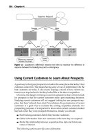
Neural networks are easily adapted for time-series analysis, as shown in
Figure 7.12. The network is trained on the time-series data, starting at the
oldest point in the data. The training then moves to the second oldest point,
and the oldest point goes to the next set of units in the input layer, and so on.
The network trains like a feed-forward, back propagation network trying to
predict the next value in the series at each step.
output
Time lag
er
value 1, time t
value 1, time t-1
value 1, time t-2
value 2, time t
value 2, time t-1
value 2, time t-2
Historical units
Hidden lay
value 1, time t+1
Figure 7.12 A time-delay neural network remembers the previous few training examples
and uses them as input into the network. The network then works like a feed-forward, back
propagation network.
470643 c07.qxd 3/8/04 11:37 AM Page 246
246 Chapter 7
Notice that the time-series network is not limited to data from just a single

time series. It can take multiple inputs. For instance, to predict the value of the
Swiss franc to U.S. dollar exchange rate, other time-series information might be
included, such as the volume of the previous day’s transactions, the U.S. dollar
to Japanese yen exchange rate, the closing value of the stock exchange, and the
day of the week. In addition, non-time-series data, such as the reported infla-
tion rate in the countries over the period of time under investigation, might
also be candidate features.
The number of historical units controls the length of the patterns that the
network can recognize. For instance, keeping 10 historical units on a network
predicting the closing price of a favorite stock will allow the network to recog-
nize patterns that occur within 2-week time periods (since exchange rates are
set only on weekdays). Relying on such a network to predict the value 3
months in the future may not be a good idea and is not recommended.
Actually, by modifying the input, a feed-forward network can be made to
work like a time-delay neural network. Consider the time series with 10 days
of history, shown in Table 7.5. The network will include two features: the day
of the week and the closing price.
Create a time series with a time lag of three requires adding new features for
the historical, lagged values. (Day-of-the-week does not need to be copied,
since it does not really change.) The result is Table 7.6. This data can now be
input into a feed-forward, back propagation network without any special sup-
port for time series.
Table 7.5 Time Series
DATA ELEMENT DAY-OF-WEEK CLOSING PRICE
1 1 $40.25
2 2 $41.00
3 3 $39.25
4 4 $39.75
5 5 $40.50
6 1 $40.50

7 2 $40.75
8 3 $41.25
9 4 $42.00
10 5 $41.50
470643 c07.qxd 3/8/04 11:37 AM Page 247
Artificial Neural Networks 247
Table 7.6 Time Series with Time Lag
PRICE PRICE PRICE
PREVIOUS PREVIOUS-1
DATA DAY-OF- CLOSING CLOSING CLOSING
ELEMENT WEEK
1 1 $40.25
2 2 $41.00 $40.25
3 3 $39.25 $41.00 $40.25
4 4 $39.75 $39.25 $41.00
5 5 $40.50 $39.75 $39.25
6 1 $40.50 $40.50 $39.75
7 2 $40.75 $40.50 $40.50
8 3 $41.25 $40.75 $40.50
9 4 $42.00 $41.25 $40.75
10 5 $41.50 $42.00 $41.25
How to Know What Is Going on
Inside a Neural Network
Neural networks are opaque. Even knowing all the weights on all the nodes
throughout the network does not give much insight into why the network
produces the results that it produces. This lack of understanding has some philo-
sophical appeal—after all, we do not understand how human consciousness
arises from the neurons in our brains. As a practical matter, though, opaqueness
impairs our ability to understand the results produced by a network.
If only we could ask it to tell us how it is making its decision in the form of

rules. Unfortunately, the same nonlinear characteristics of neural network
nodes that make them so powerful also make them unable to produce simple
rules. Eventually, research into rule extraction from networks may bring
unequivocally good results. Until then, the trained network itself is the rule,
and other methods are needed to peer inside to understand what is going on.
A technique called sensitivity analysis can be used to get an idea of how
opaque models work. Sensitivity analysis does not provide explicit rules, but
it does indicate the relative importance of the inputs to the result of the net-
work. Sensitivity analysis uses the test set to determine how sensitive the out-
put of the network is to each input. The following are the basic steps:
1. Find the average value for each input. We can think of this average
value as the center of the test set.
470643 c07.qxd 3/8/04 11:37 AM Page 248
248 Chapter 7
2. Measure the output of the network when all inputs are at their average
value.
3. Measure the output of the network when each input is modified, one at
a time, to be at its minimum and maximum values (usually –1 and 1,
respectively).
For some inputs, the output of the network changes very little for the three
values (minimum, average, and maximum). The network is not sensitive to
these inputs (at least when all other inputs are at their average value). Other
inputs have a large effect on the output of the network. The network is
sensitive to these inputs. The amount of change in the output measures the sen-
sitivity of the network for each input. Using these measures for all the inputs
creates a relative measure of the importance of each feature. Of course, this
method is entirely empirical and is looking only at each variable indepen-
dently. Neural networks are interesting precisely because they can take inter-
actions between variables into account.
There are variations on this procedure. It is possible to modify the values of

two or three features at the same time to see if combinations of features have a
particular importance. Sometimes, it is useful to start from a location other
than the center of the test set. For instance, the analysis might be repeated for
the minimum and maximum values of the features to see how sensitive the
network is at the extremes. If sensitivity analysis produces significantly differ-
ent results for these three situations, then there are higher order effects in the
network that are taking advantage of combinations of features.
When using a feed-forward, back propagation network, sensitivity analysis
can take advantage of the error measures calculated during the learning phase
instead of having to test each feature independently. The validation set is fed
into the network to produce the output and the output is compared to the
predicted output to calculate the error. The network then propagates the error
back through the units, not to adjust any weights but to keep track of the sen-
sitivity of each input. The error is a proxy for the sensitivity, determining how
much each input affects the output in the network. Accumulating these sensi-
tivities over the entire test set determines which inputs have the larger effect
on the output. In our experience, though, the values produced in this fashion
are not particularly useful for understanding the network.
Neural networks do not produce easily understood rules that explain howTIP
they arrive at a given result. Even so, it is possible to understand the relative
importance of inputs into the network by using sensitivity analysis. Sensitivity
can be a manual process where each feature is tested one at a time relative to
the other features. It can also be more automated by using the sensitivity
information generated by back propagation. In many situations, understanding
the relative importance of inputs is almost as good as having explicit rules.
470643 c07.qxd 3/8/04 11:37 AM Page 249
Artificial Neural Networks 249
Self-Organizing Maps
Self-organizing maps (SOMs) are a variant of neural networks used for undirected
data mining tasks such as cluster detection. The Finnish researcher Dr. Tuevo

Kohonen invented self-organizing maps, which are also called Kohonen Net-
works. Although used originally for images and sounds, these networks can also
recognize clusters in data. They are based on the same underlying units as feed-
forward, back propagation networks, but SOMs are quite different in two respects.
They have a different topology and the back propagation method of learning is
no longer applicable. They have an entirely different method for training.
What Is a Self-Organizing Map?
The self-organizing map (SOM), an example of which is shown in Figure 7.13, is
a neural network that can recognize unknown patterns in the data. Like the
networks we’ve already looked at, the basic SOM has an input layer and an
output layer. Each unit in the input layer is connected to one source, just as in
the networks for predictive modeling. Also, like those networks, each unit in
the SOM has an independent weight associated with each incoming connec-
tion (this is actually a property of all neural networks). However, the similar-
ity between SOMs and feed-forward, back propagation networks ends here.
The output layer consists of many units instead of just a handful. Each of the
units in the output layer is connected to all of the units in the input layer. The
output layer is arranged in a grid, as if the units were in the squares on a
checkerboard. Even though the units are not connected to each other in this
layer, the grid-like structure plays an important role in the training of the
SOM, as we will see shortly.
How does an SOM recognize patterns? Imagine one of the booths at a carni-
val where you throw balls at a wall filled with holes. If the ball lands in one of
the holes, then you have your choice of prizes. Training an SOM is like being
at the booth blindfolded and initially the wall has no holes, very similar to the
situation when you start looking for patterns in large amounts of data and
don’t know where to start. Each time you throw the ball, it dents the wall a lit-
tle bit. Eventually, when enough balls land in the same vicinity, the indentation
breaks through the wall, forming a hole. Now, when another ball lands at that
location, it goes through the hole. You get a prize—at the carnival, this is a

cheap stuffed animal, with an SOM, it is an identifiable cluster.
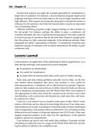
Figure 7.14 shows how this works for a simple SOM. When a member of the
training set is presented to the network, the values flow forward through the
network to the units in the output layer. The units in the output layer compete
with each other, and the one with the highest value “wins.” The reward is to
adjust the weights leading up to the winning unit to strengthen in the response
to the input pattern. This is like making a little dent in the network.
470643 c07.qxd 3/8/04 11:37 AM Page 250
250 Chapter 7
The output units compete with
each other for the output of the
network.
The output layer is laid out like a
grid. Each unit is connected to
all the input units, but not to each
other.
The input layer is connected to
the inputs.
Figure 7.13 The self-organizing map is a special kind of neural network that can be used
to detect clusters.
There is one more aspect to the training of the network. Not only are the
weights for the winning unit adjusted, but the weights for units in its immedi-
ate neighborhood are also adjusted to strengthen their response to the inputs.
This adjustment is controlled by a neighborliness parameter that controls the
size of the neighborhood and the amount of adjustment. Initially, the neigh-
borhood is rather large, and the adjustments are large. As the training contin-
ues, the neighborhoods and adjustments decrease in size. Neighborliness
actually has several practical effects. One is that the output layer behaves more
like a connected fabric, even though the units are not directly connected to
each other. Clusters similar to each other should be closer together than more

dissimilar clusters. More importantly, though, neighborliness allows for a
group of units to represent a single cluster. Without this neighborliness, the
network would tend to find as many clusters in the data as there are units in
the output layer—introducing bias into the cluster detection.
470643 c07.qxd 3/8/04 11:37 AM Page 251
Artificial Neural Networks 251
0.1
0.2
0.7
0.2
0.6
0.6
0.1
0.9
0.4
0.2
0.1
0.8
The winning output
unit and its path
Figure 7.14 An SOM finds the output unit that does the best job of recognizing a particular
input.
Typically, a SOM identifies fewer clusters than it has output units. This is
inefficient when using the network to assign new records to the clusters, since
the new inputs are fed through the network to unused units in the output
layer. To determine which units are actually used, we apply the SOM to the
validation set. The members of the validation set are fed through the network,
keeping track of the winning unit in each case. Units with no hits or with very
few hits are discarded. Eliminating these units increases the run-time perfor-
mance of the network by reducing the number of calculations needed for new

instances.
Once the final network is in place—with the output layer restricted only to
the units that identify specific clusters—it can be applied to new instances. An
470643 c07.qxd 3/8/04 11:37 AM Page 252
252 Chapter 7
unknown instance is fed into the network and is assigned to the cluster at the
output unit with the largest weight. The network has identified clusters, but
we do not know anything about them. We will return to the problem of identi-
fying clusters a bit later.
The original SOMs used two-dimensional grids for the output layer. This
was an artifact of earlier research into recognizing features in images com-
posed of a two-dimensional array of pixel values. The output layer can really
have any structure—with neighborhoods defined in three dimensions, as a
network of hexagons, or laid out in some other fashion.
Example: Finding Clusters
A large bank is interested in increasing the number of home equity loans that
it sells, which provides an illustration of the practical use of clustering. The
bank decides that it needs to understand customers that currently have home
equity loans to determine the best strategy for increasing its market share. To
start this process, demographics are gathered on 5,000 customers who have
home equity loans and 5,000 customers who do not have them. Even though
the proportion of customers with home equity loans is less than 50 percent, it
is a good idea to have equal weights in the training set.
The data that is gathered has fields like the following:
■■ Appraised value of house
■■ Amount of credit available
■■ Amount of credit granted
■■ Age
■■ Marital status
■■ Number of children

■■ Household income
This data forms a good training set for clustering. The input values are
mapped so they all lie between –1 and +1; these are used to train an SOM. The
network identifies five clusters in the data, but it does not give any informa-
tion about the clusters. What do these clusters mean?
A common technique to compare different clusters that works particularly
well with neural network techniques is the average member technique. Find the
most average member of each of the clusters—the center of the cluster. This is
similar to the approach used for sensitivity analysis. To do this, find the aver-
age value for each feature in each cluster. Since all the features are numbers,
this is not a problem for neural networks.
For example, say that half the members of a cluster are male and half are
female, and that male maps to –1.0 and female to +1.0. The average member
for this cluster would have a value of 0.0 for this feature. In another cluster,
TEAMFLY

Team-Fly
®

there may be nine females for every male. For this cluster, the average member
would have a value of 0.8. This averaging works very well with neural net-
works since all inputs have to be mapped into a numeric range.
TIP Self-organizing maps, a type of neural network, can identify clusters but
they do not identify what makes the members of a cluster similar to each other.
A powerful technique for comparing clusters is to determine the center or
average member in each cluster. Using the test set, calculate the average value
for each feature in the data. These average values can then be displayed in the
same graph to determine the features that make a cluster unique.
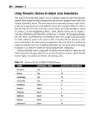
These average values can then be plotted using parallel coordinates as in
Figure 7.15, which shows the centers of the five clusters identified in the bank-
ing example. In this case, the bank noted that one of the clusters was particu-
larly interesting, consisting of married customers in their forties with children.
A bit more investigation revealed that these customers also had children in
their late teens. Members of this cluster had more home equity lines than
members of other clusters.
Figure 7.15 The centers of five clusters are compared on the same graph. This simple
visualization technique (called parallel coordinates) helps identify interesting clusters.
Available

Credit
Credit
Balance
Age Marital
Status
Num
Children
Income
-1.0
-0.8
-0.6
-0.4
-0.2
0.0
0.2
0.4
0.6
0.8
1.0
This cluster looks interesting. High-income customers
with children in the middle age group who are taking
out large loans.
Artificial Neural Networks 253
470643 c07.qxd 3/8/04 11:37 AM Page 253
470643 c07.qxd 3/8/04 11:37 AM Page 254
254 Chapter 7
The story continues with the Marketing Department of the bank concluding
that these people had taken out home equity loans to pay college tuition fees.
The department arranged a marketing program designed specifically for this
market, selling home equity loans as a means to pay for college education. The

results from this campaign were disappointing. The marketing program was
not successful.
Since the marketing program failed, it may seem as though the clusters did
not live up to their promise. In fact, the problem lay elsewhere. The bank had
initially only used general customer information. It had not combined infor-
mation from the many different systems servicing its customers. The bank
returned to the problem of identifying customers, but this time it included
more information—from the deposits system, the credit card system, and
so on.
The basic methods remained the same, so we will not go into detail about
the analysis. With the additional data, the bank discovered that the cluster of
customers with college-age children did actually exist, but a fact had been
overlooked. When the additional data was included, the bank learned that the
customers in this cluster also tended to have business accounts as well as per-
sonal accounts. This led to a new line of thinking. When the children leave
home to go to college, the parents now have the opportunity to start a new
business by taking advantage of the equity in their home.
With this insight, the bank created a new marketing program targeted at the
parents, about starting a new business in their empty nest. This program suc-
ceeded, and the bank saw improved performance from its home equity loans
group. The lesson of this case study is that, although SOMs are powerful tools
for finding clusters, neural networks really are only as good as the data that
goes into them.
Lessons Learned
Neural networks are a versatile data mining tool. Across a large number of
industries and a large number of applications, neural networks have proven
themselves over and over again. These results come in complicated domains,
such as analyzing time series and detecting fraud, that are not easily amenable
to other techniques. The largest neural network developed for production is
probably the system that AT&T developed for reading numbers on checks. This

neural network has hundreds of thousands of units organized into seven layers.
Their foundation is based on biological models of how brains work.
Although predating digital computers, the basic ideas have proven useful. In
biology, neurons fire after their inputs reach a certain threshold. This model
470643 c07.qxd 3/8/04 11:37 AM Page 255
Artificial Neural Networks 255
can be implemented on a computer as well. The field has really taken off since
the 1980s, when statisticians started to use them and understand them better.
A neural network consists of artificial neurons connected together. Each
neuron mimics its biological counterpart, taking various inputs, combining
them, and producing an output. Since digital neurons process numbers, the
activation function characterizes the neuron. In most cases, this function takes
the weighted sum of its inputs and applies an S-shaped function to it. The
result is a node that sometimes behaves in a linear fashion, and sometimes
behaves in a nonlinear fashion—an improvement over standard statistical
techniques.
The most common network is the feed-forward network for predictive mod-
eling. Although originally a breakthrough, the back propagation training
method has been replaced by other methods, notably conjugate gradient.
These networks can be used for both categorical and continuous inputs. How-
ever, neural networks learn best when input fields have been mapped to the
range between –1 and +1. This is a guideline to help train the network. Neural
networks still work when a small amount of data falls outside the range and
for more limited ranges, such as 0 to 1.
Neural networks do have several drawbacks. First, they work best when
there are only a few input variables, and the technique itself does not help
choose which variables to use. Variable selection is an issue. Other techniques,
such as decision trees can come to the rescue. Also, when training a network,
there is no guarantee that the resulting set of weights is optimal. To increase
confidence in the result, build several networks and take the best one.

Perhaps the biggest problem, though, is that a neural network cannot
explain what it is doing. Decision trees are popular because they can provide a
list of rules. There is no way to get an accurate set of rules from a neural net-
work. A neural network is explained by its weights, and a very complicated
mathematical formula. Unfortunately, making sense of this is beyond our
human powers of comprehension.
Variations on neural networks, such as self-organizing maps, extend the
technology to undirected clustering. Overall neural networks are very power-
ful and can produce good models; they just can’t tell us how they do it.
470643 c07.qxd 3/8/04 11:37 AM Page 256
470643 c08.qxd 3/8/04 11:14 AM Page 257
Nearest Neighbor Approaches:
Memory-Based Reasoning and
8
Collaborative Filtering
CHAPTER
You hear someone speak and immediately guess that she is from Australia.
Why? Because her accent reminds you of other Australians you have met. Or
you try a new restaurant expecting to like it because a friend with good taste
recommended it. Both cases are examples of decisions based on experience.
When faced with new situations, human beings are guided by memories of
similar situations they have experienced in the past. That is the basis for the
data mining techniques introduced in this chapter.
Nearest neighbor techniques are based on the concept of similarity.
Memory-based reasoning (MBR) results are based on analogous situations in
the past—much like deciding that a new friend is Australian based on past
examples of Australian accents. Collaborative filtering adds more information,
using not just the similarities among neighbors, but also their preferences. The
restaurant recommendation is an example of collaborative filtering.
Central to all these techniques is the idea of similarity. What really makes

situations in the past similar to a new situation? Along with finding the simi-
lar records from the past, there is the challenge of combining the informa-
tion from the neighbors. These are the two key concepts for nearest neighbor
approaches.
This chapter begins with an introduction to MBR and an explanation of how
it works. Since measures of distance and similarity are important to nearest
neighbor techniques, there is a section on distance metrics, including a discus-
sion of the meaning of distance for data types, such as free text, that have no
257
470643 c08.qxd 3/8/04 11:14 AM Page 258
258 Chapter 8
obvious geometric interpretation. The ideas of MBR are illustrated through a
case study showing how MBR has been used to attach keywords to news sto-
ries. The chapter then looks at collaborative filtering, a popular approach to
making recommendations, especially on the Web. Collaborative filtering is
also based on nearest neighbors, but with a slight twist—instead of grouping
restaurants or movies into neighborhoods, it groups the people recommend-
ing them.
Memory Based Reasoning
The human ability to reason from experience depends on the ability to recog-
nize appropriate examples from the past. A doctor diagnosing diseases, a
claims analyst flagging fraudulent insurance claims, and a mushroom hunter
spotting Morels are all following a similar process. Each first identifies similar
cases from experience and then applies what their knowledge of those cases to
the problem at hand. This is the essence of memory-based reasoning. A data-
base of known records is searched to find preclassified records similar to a new
record. These neighbors are used for classification and estimation.
Applications of MBR span many areas:
Fraud detection. New cases of fraud are likely to be similar to known
cases. MBR can find and flag them for further investigation.

Customer response prediction. The next customers likely to respond
to an offer are probably similar to previous customers who have
responded. MBR can easily identify the next likely customers.
Medical treatments. The most effective treatment for a given patient is
probably the treatment that resulted in the best outcomes for similar
patients. MBR can find the treatment that produces the best outcome.
Classifying responses. Free-text responses, such as those on the U.S. Cen-
sus form for occupation and industry or complaints coming from cus-
tomers, need to be classified into a fixed set of codes. MBR can process
the free-text and assign the codes.
One of the strengths of MBR is its ability to use data “as is.” Unlike other data
mining techniques, it does not care about the format of the records. It only cares
about the existence of two operations: A distance function capable of calculating
a distance between any two records and a combination function capable of com-
bining results from several neighbors to arrive at an answer. These functions
are readily defined for many kinds of records, including records with complex
or unusual data types such as geographic locations, images, and free text that
470643 c08.qxd 3/8/04 11:14 AM Page 259
Memory-Based Reasoning and Collaborative Filtering 259
are usually difficult to handle with other analysis techniques. A case study
later in the chapter shows MBR’s successful application to the classification of
news stories—an example that takes advantage of the full text of the news
story to assign subject codes.
Another strength of MBR is its ability to adapt. Merely incorporating new
data into the historical database makes it possible for MBR to learn about new
categories and new definitions of old ones. MBR also produces good results
without a long period devoted to training or to massaging incoming data into
the right format.
These advantages come at a cost. MBR tends to be a resource hog since a
large amount of historical data must be readily available for finding neighbors.

Classifying new records can require processing all the historical records to find
the most similar neighbors—a more time-consuming process than applying an
already-trained neural network or an already-built decision tree. There is also
the challenge of finding good distance and combination functions, which often
requires a bit of trial and error and intuition.
Example: Using MBR to Estimate
Rents in Tuxedo, New York
The purpose of this example is to illustrate how MBR works by estimating the
cost of renting an apartment in the target town by combining data on rents in
several similar towns—its nearest neighbors.
MBR works by first identifying neighbors and then combining information
from them. Figure 8.1 illustrates the first of these steps. The goal is to make
predictions about the town of Tuxedo in Orange County, New York by looking
at its neighbors. Not its geographic neighbors along the Hudson and Delaware
rivers, rather its neighbors based on descriptive variables—in this case, popu-
lation and median home value. The scatter plot shows New York towns
arranged by these two variables. Figure 8.1 shows that measured this way,
Brooklyn and Queens are close neighbors, and both are far from Manhattan.
Although Manhattan is nearly as populous as Brooklyn and Queens, its home
prices put it in a class by itself.
TIP Neighborhoods can be found in many dimensions. The choice of
dimensions determines which records are close to one another. For some
purposes, geographic proximity might be important. For other purposes home
price or average lot size or population density might be more important. The
choice of dimensions and the choice of a distance metric are crucial to any
nearest-neighbor approach.
470643 c08.qxd 3/8/04 11:14 AM Page 260
260 Chapter 8
The first stage of MBR finds the closest neighbor on the scatter plot shown
in Figure 8.1. Then the next closest neighbor is found, and so on until the

desired number are available. In this case, the number of neighbors is two and
the nearest ones turn out to be Shelter Island (which really is an island) way
out by the tip of Long Island’s North Fork, and North Salem, a town in North-
ern Westchester near the Connecticut border. These towns fall at about the
middle of a list sorted by population and near the top of one sorted by home
value. Although they are many miles apart, along these two dimensions, Shel-
ter Island and North Salem are very similar to Tuxedo.
Once the neighbors have been located, the next step is to combine informa-
tion from the neighbors to infer something about the target. For this example,
the goal is to estimate the cost of renting a house in Tuxedo. There is more than
one reasonable way to combine data from the neighbors. The census provides
information on rents in two forms. Table 8.1 shows what the 2000 census
reports about rents in the two towns selected as neighbors. For each town,
there is a count of the number of households paying rent in each of several
price bands as well as the median rent for each town. The challenge is to figure
out how best to use this data to characterize rents in the neighbors and then
how to combine information from the neighbors to come up with an estimate
that characterizes rents in Tuxedo in the same way.
Tuxedo’s nearest neighbors, the towns of North Salem and Shelter Island,
have quite different distributions of rents even though the median rents are
similar. In Shelter Island, a plurality of homes, 34.6 percent, rent in the $500 to
$750 range. In the town of North Salem, the largest number of homes, 30.9 per-
cent, rent in the $1,000 to $1,500 range. Furthermore, while only 3.1 percent of
homes in Shelter Island rent for over $1,500, 24.2 percent of homes in North
Salem do. On the other hand, at $804, the median rent in Shelter Island is above
the $750 ceiling of the most common range, while the median rent in North
Salem, $1,150, is below the floor of the most common range for that town. If
the average rent were available, it too would be a good candidate for character-
izing the rents in the various towns.
Table 8.1 The Neighbors

(%) (%) (%) (%) (%) (%)
RENT RENT RENT RENT RENT NO
POPULA- MEDIAN <$500 $750 $1500 $1000 >$1500 RENT
TOWN TION RENT
Shelter 2228 $804 3.1 34.6 31.4 10.7 3.1 17
Island
North 5173 $1150 3 10.2 21.6 30.9 24.2 10.2
Salem
Figure 8.1
Based on 2000 census population and home value, the town of T
uxedo
in Orange County has Shelter Island and North Salem as its two nearest neighbors.
Population vs Home Value
0
200000
400000
600000
800000
1000000
1200000
0246
81
01
21
41
6
Log Population
Median Home Value
Shelter Island,
Suffolk

North Salem,
Westchester
Tuxedo,
Orange
Manhattan,
New York
Brooklyn,
Kings
Queens,
Queens
Scarsdale,
Westchester
Memory-Based Reasoning and Collaborative Filtering 261
470643 c08.qxd 3/8/04 11:14 AM Page 261
470643 c08.qxd 3/8/04 11:14 AM Page 262
262 Chapter 8
One possible combination function would be to average the most common
rents of the two neighbors. Since only ranges are available, we use the mid-
points. For Shelter Island, the midpoint of the most common range is $1,000.
For North Salem, it is $1,250. Averaging the two leads to an estimate for rent in
Tuxedo of $1,125. Another combination function would pick the point midway
between the two median rents. This second method leads to an estimate of
$977 for rents in Tuxedo.
As it happens, a plurality of rents in Tuxedo are in the $1,000 to $1,500 range
with the midpoint at $1,250. The median rent in Tuxedo is $907. So, averaging
the medians slightly overestimates the median rent in Tuxedo and averaging
the most common rents slightly underestimates the most common rent in
Tuxedo. It is hard to say which is better. The moral is that there is not always
an obvious “best” combination function.
Challenges of MBR

In the simple example just given, the training set consisted of all towns in New
York, each described by a handful of numeric fields such as the population,
median home value, and median rent. Distance was determined by placement
on a scatter plot with axes scaled to appropriate ranges, and the number of
neighbors arbitrarily set to two. The combination function was a simple
average.
All of these choices seem reasonable. In general, using MBR involves several
choices:
1. Choosing an appropriate set of training records
2. Choosing the most efficient way to represent the training records
3. Choosing the distance function, the combination function, and the
number of neighbors
Let’s look at each of these in turn.
Choosing a Balanced Set of Historical Records
The training set is a set of historical records. It needs to provide good coverage
of the population so that the nearest neighbors of an unknown record are use-
ful for predictive purposes. A random sample may not provide sufficient cov-
erage for all values. Some categories are much more frequent than others and
the more frequent categories dominate the random sample.
For instance, fraudulent transactions are much rarer than non-fraudulent
transactions, heart disease is much more common than liver cancer, news sto-
ries about the computer industry more common than about plastics, and so on.
TEAMFLY

Team-Fly
®

470643 c08.qxd 3/8/04 11:14 AM Page 263
Memory-Based Reasoning and Collaborative Filtering 263
To achieve balance, the training set should, if possible, contain roughly equal
numbers of records representing the different categories.
TIP When selecting the training set for MBR, be sure that each category has
roughly the same number of records supporting it. As a general rule of thumb,
several dozen records for each category are a minimum to get adequate
support and hundreds or thousands of examples are not unusual.
Representing the Training Data
The performance of MBR in making predictions depends on how the training
set is represented. The scatter plot approach illustrated in Figure 8.2 works for

two or three variables and a small number of records, but it does not scale well.
The simplest method for finding nearest neighbors requires finding the dis-
tance from the unknown case to each of the records in the training set and
choosing the training records with the smallest distances. As the number of
records grows, the time needed to find the neighbors for a new record grows
quickly.
This is especially true if the records are stored in a relational database. In this
case, the query looks something like:
SELECT distance(),rec.category
FROM historical_records rec
ORDER BY 1 ASCENDING;
The notation distance() fills in for whatever the particular distance function
happens to be. In this case, all the historical records need to be sorted in order
to get the handful needed for the nearest neighbors. This requires a full-table
scan plus a sort—quite an expensive couple of operations. It is possible to elim-
inate the sort by walking through table and keeping another table of the near-
est, inserting and deleting records as appropriate. Unfortunately, this approach
is not readily expressible in SQL without using a procedural language.
The performance of relational databases is pretty good nowadays. The chal-
lenge with scoring data for MBR is that each case being scored needs to be
compared against every case in the database. Scoring a single new record does
not take much time, even when there are millions of historical records. How-
ever, scoring many new records can have poor performance.
Another way to make MBR more efficient is to reduce the number of records
in the training set. Figure 8.2 shows a scatter plot for categorical data. This
graph has a well-defined boundary between the two regions. The points above
the line are all diamonds and those below the line are all circles. Although this
graph has forty points in it, most of the points are redundant. That is, they are
not really necessary for classification purposes.
470643 c08.qxd 3/8/04 11:14 AM Page 264

264 Chapter 8
1
0.9
0.8
0.7
0.6
0.5
0.4
0.3
0.2
0.1
0
0 0.2 0.4 0.6 0.8 1
Figure 8.2 Perhaps the cleanest training set for MBR is one that divides neatly into two
disjoint sets.
Figure 8.3 shows that only eight points in it are needed to get the same
results. Given that the size of the training set has such a large influence on the
performance of MBR, being able to reduce the size is a significant performance
boost.
How can this reduced set of records be found? The most practical method is
to look for clusters containing records belonging to different categories. The
centers of the clusters can then be used as a reduced set. This works well when
the different categories are quite separate. However, when there is some over-
lap and the categories are not so well-defined, using clusters to reduce the size
of the training set can cause MBR to produce poor results. Finding an optimal
set of “support records” has been an area of recent research. When such an
optimal set can be found, the historical records can sometimes be reduced to
the level where they fit inside a spreadsheet, making it quite efficient to apply
MBR to new records on less powerful machines.
470643 c08.qxd 3/8/04 11:14 AM Page 265

Memory-Based Reasoning and Collaborative Filtering 265
1
0.9
0.8
0.7
0.6
0.5
0.4
0.3
0.2
0.1
0
0 0.2 0.4 0.6 0.8 1
Figure 8.3 This smaller set of points returns the same results as in Figure 8.2 using MBR.
Determining the Distance Function, Combination
Function, and Number of Neighbors
The distance function, combination function, and number of neighbors are the
key ingredients in using MBR. The same set of historical records can prove
very useful or not at all useful for predictive purposes, depending on these cri-
teria. Fortunately, simple distance functions and combination functions usu-
ally work quite well. Before discussing these issues in detail, let’s look at a
detailed case study.
Case Study: Classifying News Stories
This case study uses MBR to assign classification codes to news stories and is
based on work conducted by one of the authors. The results from this case
study show that MBR can perform as well as people on a problem involving
hundreds of categories and data on a difficult-to-use type of data, free-text.
1
1
This case study is a summarization of research conducted by one of the authors. Complete details

are available in the article “Classifying News Stories using Memory Based Reasoning,” by David
Waltz, Brij Masand, and Gordon Linoff, in Proceedings, SIGIR ‘92, published by ACM Press.
470643 c08.qxd 3/8/04 11:14 AM Page 266
266 Chapter 8
What Are the Codes?
The classification codes are keywords used to describe the content of news sto-
ries. These codes are added to stories by a news retrieval service to help users
search for stories of interest. They help automate the process of routing partic-
ular stories to particular customers and help implement personalized profiles.
For instance, an industry analyst who specializes in the automotive industry
(or anyone else with an interest in the topic) can simplify searches by looking
for documents with the “automotive industry” code. Because knowledgeable
experts, also known as editors, set up the codes, the right stories are retrieved.
Editors or expert systems have traditionally assigned these codes. This case
study investigated the use of MBR for this purpose.
The codes used in this study fall into six categories:
■■ Government Agency
■■ Industry
■■ Market Sector
■■ Product
■■ Region
■■ Subject
The data contained 361 separate codes, distributed as follows in the training
set (Table 8.2).
The number and types of codes assigned to stories varied. Almost all the
stories had region and subject codes—and, on average, almost three region
codes per story. At the other extreme, relatively few stories contained govern-
ment and product codes, and such stories rarely had more than one such code.
Table 8.2 Six Types of Codes Used to Classify News Stories
CATEGORY # CODES # DOCS # OCCURRENCES

Government (G/) 28 3,926 4,200
Industry (I/) 112 38,308 57,430
Market Sector (M/) 9 38,562 42,058
Product (P/) 21 2,242 2,523
Region (R/) 121 47,083 116,358
Subject (N/) 70 41,902 52,751
470643 c08.qxd 3/8/04 11:14 AM Page 267
Memory-Based Reasoning and Collaborative Filtering 267
Applying MBR
This section explains how MBR facilitated assigning codes to news stories for
a news service. The important steps were:
1. Choosing the training set
2. Determining the distance function
3. Choosing the number of nearest neighbors
4. Determining the combination function
The following sections discuss each of these steps in turn.
Choosing the Training Set
The training set consisted of 49,652 news stories, provided by the news
retrieval service for this purpose. These stories came from about three months
of news and from almost 100 different sources. Each story contained, on aver-
age, 2,700 words and had eight codes assigned to it. The training set was not
specially created, so the frequency of codes in the training set varied a great
deal, mimicking the overall frequency of codes in news stories in general.
Although this training set yielded good results, a better-constructed training
set with more examples of the less common codes would probably have per-
formed even better.
Choosing the Distance Function
The next step is choosing the distance function. In this case, a distance function
already existed, based on a notion called relevance feedback that measures the
similarity of two documents based on the words they contain. Relevance feed-

back, which is described more fully in the sidebar, was originally designed to
return documents similar to a given document, as a way of refining searches.
The most similar documents are the neighbors used for MBR.
Choosing the Combination Function
The next decision is the combination function. Assigning classification codes
to news stories is a bit different from most classification problems. Most classi-
fication problems are looking for the single best solution. However, news sto-
ries can have multiple codes, even from the same category. The ability to adapt
MBR to this problem highlights its flexibility.
470643 c08.qxd 3/8/04 11:14 AM Page 268
268 Chapter 8
to one they already have. (Hubs and authorities, another method for improving
database and returns those that are most similar—along with a measure of
follows:
so common, they provide little information to distinguish between
documents.
searchable terms.
identified (automatically) and included in the dictionary of searchable
feedback score to a function suitable for measuring the “distance” between
news stories:
d
classification
(A,B) = 1 –
score(A,B)
score(A,A)
not a true distance function because d(A,B) is not the same as d(B,A), but it
works well enough.
USING RELEVANCE FEEDBACK TO CREATE A DISTANCE FUNCTION
Relevance feedback is a powerful technique that allows users to refine
searches on text databases by asking the database to return documents similar

search results on hyperlinked web pages, is described in Chapter 10.) In the
course of doing this, the text database scores all the other documents in the
similarity. This is the relevance feedback score, which can be used as the basis
for a distance measure for MBR.
In the case study, the calculation of the relevance feedback score went as
1. Common, non-content-bearing words, such as “it,” “and,” and “of,” were
removed from the text of all stories in the training set. A total of 368
words in this category were identified and removed.
2. The next most common words, accounting for 20 percent of the words
in the database, were removed from the text. Because these words are
3. The remaining words were collected into a dictionary of
Each was assigned a weight inversely proportional to its frequency in the
database. The particular weight was the negative of the base 2 log of the
term’s frequency in the training set.
4. Capitalized word pairs, such as “United States” and “New Mexico,” were
terms.
5. To calculate the relevance feedback score for two stories, the weights of
the searchable terms in both stories were added together. The algorithm
used for this case study included a bonus when searchable terms ap-
peared in close proximity in both stories.
The relevance feedback score is an example of the adaptation of an already-
existing function for use as a distance function. However, the score itself does
not quite fit the definition of a distance function. In particular, a score of 0
indicates that two stories have no words in common, instead of implying that
the stories are identical. The following transformation converts the relevance
This is the function used to find the nearest neighbors. Actually, even this is