John wiley sons data mining techniques for marketing sales_4 pdf

470643 c03.qxd 3/8/04 11:09 AM Page 74
74 Chapter 3
When missing values must be replaced, the best approach is to impute them
by creating a model that has the missing value as its target variable.
Values with Meanings That Change over Time
When data comes from several different points in history, it is not uncommon
for the same value in the same field to have changed its meaning over time.
Credit class “A” may always be the best, but the exact range of credit scores
that get classed as an “A” may change from time to time. Dealing with this
properly requires a well-designed data warehouse where such changes in
meaning are recorded so a new variable can be defined that has a constant
meaning over time.
Inconsistent Data Encoding
When information on the same topic is collected from multiple sources, the
various sources often represent the same data different ways. If these differ-
ences are not caught, they add spurious distinctions that can lead to erroneous
conclusions. In one call-detail analysis project, each of the markets studied had
a different way of indicating a call to check one’s own voice mail. In one city, a
call to voice mail from the phone line associated with that mailbox was
recorded as having the same origin and destination numbers. In another city,
the same situation was represented by the presence of a specific nonexistent
number as the call destination. In yet another city, the actual number dialed to
reach voice mail was recorded. Understanding apparent differences in voice
mail habits between cities required putting the data in a common form.
The same data set contained multiple abbreviations for some states and, in
some cases, a particular city was counted separately from the rest of the state.
If issues like this are not resolved, you may find yourself building a model of
calling patterns to California based on data that excludes calls to Los Angeles.
Step Six: Transform Data to Bring
Information to the Surface
Once the data has been assembled and major data problems fixed, the data

must still be prepared for analysis. This involves adding derived fields to
bring information to the surface. It may also involve removing outliers, bin-
ning numeric variables, grouping classes for categorical variables, applying
transformations such as logarithms, turning counts into proportions, and the
470643 c03.qxd 3/8/04 11:09 AM Page 75
Data Mining Methodology and Best Practices 75
like. Data preparation is such an important topic that our colleague Dorian
Pyle has written a book about it, Data Preparation for Data Mining (Morgan
Kaufmann 1999), which should be on the bookshelf of every data miner. In this
book, these issues are addressed in Chapter 17. Here are a few examples of
such transformations.
Capture Trends
Most corporate data contains time series. Monthly snapshots of billing informa-
tion, usage, contacts, and so on. Most data mining algorithms do not understand
time series data. Signals such as “three months of declining revenue” cannot be
spotted treating each month’s observation independently. It is up to the data
miner to bring trend information to the surface by adding derived variables
such as the ratio of spending in the most recent month to spending the month
before for a short-term trend and the ratio of the most recent month to the same
month a year ago for a long-term trend.
Create Ratios and Other Combinations of Variables
Trends are one example of bringing information to the surface by combining
multiple variables. There are many others. Often, these additional fields are
derived from the existing ones in ways that might be obvious to a knowledge-
able analyst, but are unlikely to be considered by mere software. Typical exam-
ples include:
obesity_index = height
2
/ weight
PE = price / earnings

pop_density = population / area
rpm = revenue_passengers * miles
Adding fields that represent relationships considered important by experts
in the field is a way of letting the mining process benefit from that expertise.
Convert Counts to Proportions
Many datasets contain counts or dollar values that are not particularly inter-
esting in themselves because they vary according to some other value. Larger
households spend more money on groceries than smaller households. They
spend more money on produce, more money on meat, more money on pack-
aged goods, more money on cleaning products, more money on everything.
So comparing the dollar amount spent by different households in any one
470643 c03.qxd 3/8/04 11:09 AM Page 76
76 Chapter 3
category, such as bakery, will only reveal that large households spend more. It
is much more interesting to compare the proportion of each household’s spend-
ing that goes to each category.
The value of converting counts to proportions can be seen by comparing
two charts based on the NY State towns dataset. Figure 3.9 compares the count
of houses with bad plumbing to the prevalence of heating with wood. A rela-
tionship is visible, but it is not strong. In Figure 3.10, where the count of houses
with bad plumbing has been converted into the proportion of houses with bad
plumbing, the relationship is much stronger. Towns where many houses have
bad plumbing also have many houses heated by wood. Does this mean that
wood smoke destroys plumbing? It is important to remember that the patterns
that we find determine correlation, not causation.
Figure 3.9 Chart comparing count of houses with bad plumbing to prevalence of heating
with wood.
470643 c03.qxd 3/8/04 11:09 AM Page 77
Data Mining Methodology and Best Practices 77
Figure 3.10 Chart comparing proportion of houses with bad plumbing to prevalence of

heating with wood.
Step Seven: Build Models
The details of this step vary from technique to technique and are described in
the chapters devoted to each data mining method. In general terms, this is the
step where most of the work of creating a model occurs. In directed data min-
ing, the training set is used to generate an explanation of the independent or
target variable in terms of the independent or input variables. This explana-
tion may take the form of a neural network, a decision tree, a linkage graph, or
some other representation of the relationship between the target and the other
fields in the database. In undirected data mining, there is no target variable.
The model finds relationships between records and expresses them as associa-
tion rules or by assigning them to common clusters.
Building models is the one step of the data mining process that has been
truly automated by modern data mining software. For that reason, it takes up
relatively little of the time in a data mining project.
470643 c03.qxd 3/8/04 11:09 AM Page 78
78 Chapter 3
Step Eight: Assess Models
This step determines whether or not the models are working. A model assess-
ment should answer questions such as:
■■ How accurate is the model?
■■ How well does the model describe the observed data?
■■ How much confidence can be placed in the model’s predictions?
■■ How comprehensible is the model?
Of course, the answer to these questions depends on the type of model that
was built. Assessment here refers to the technical merits of the model, rather
than the measurement phase of the virtuous cycle.
Assessing Descriptive Models
The rule, If (state=’MA)’ then heating source is oil, seems more descriptive
than the rule, If (area=339 OR area=351 OR area=413 OR area=508 OR

area=617 OR area=774 OR area=781 OR area=857 OR area=978) then heating
source is oil. Even if the two rules turn out to be equivalent, the first one seems
more expressive.
Expressive power may seem purely subjective, but there is, in fact, a theo-
retical way to measure it, called the minimum description length or MDL. The
minimum description length for a model is the number of bits it takes to
encode both the rule and the list of all exceptions to the rule. The fewer bits
required, the better the rule. Some data mining tools use MDL to decide which
sets of rules to keep and which to weed out.
Assessing Directed Models
Directed models are assessed on their accuracy on previously unseen data.
Different data mining tasks call for different ways of assessing performance of
the model as a whole and different ways of judging the likelihood that the
model yields accurate results for any particular record.
Any model assessment is dependent on context; the same model can look
good according to one measure and bad according to another. In the academic
field of machine learning—the source of many of the algorithms used for data
mining—researchers have a goal of generating models that can be understood
in their entirety. An easy-to-understand model is said to have good “mental
fit.” In the interest of obtaining the best mental fit, these researchers often
prefer models that consist of a few simple rules to models that contain many
such rules, even when the latter are more accurate. In a business setting, such
470643 c03.qxd 3/8/04 11:09 AM Page 79
Data Mining Methodology and Best Practices 79
explicability may not be as important as performance—or may be more
important.
Model assessment can take place at the level of the whole model or at the
level of individual predictions. Two models with the same overall accuracy
may have quite different levels of variance among the individual predictions.
A decision tree, for instance, has an overall classification error rate, but each

branch and leaf of the tree also has an error rate as well.
Assessing Classifiers and Predictors
For classification and prediction tasks, accuracy is measured in terms of the
error rate, the percentage of records classified incorrectly. The classification
error rate on the preclassified test set is used as an estimate of the expected error
rate when classifying new records. Of course, this procedure is only valid if the
test set is representative of the larger population.
Our recommended method of establishing the error rate for a model is to
measure it on a test dataset taken from the same population as the training and
validation sets, but disjointed from them. In the ideal case, such a test set
would be from a more recent time period than the data in the model set; how-
ever, this is not often possible in practice.
A problem with error rate as an assessment tool is that some errors are
worse than others. A familiar example comes from the medical world where a
false negative on a test for a serious disease causes the patient to go untreated
with possibly life-threatening consequences whereas a false positive only
leads to a second (possibly more expensive or more invasive) test. A confusion
matrix or correct classification matrix, shown in Figure 3.11, can be used to sort
out false positives from false negatives. Some data mining tools allow costs to
be associated with each type of misclassification so models can be built to min-
imize the cost rather than the misclassification rate.
Assessing Estimators
For estimation tasks, accuracy is expressed in terms of the difference between
the predicted score and the actual measured result. Both the accuracy of any
one estimate and the accuracy of the model as a whole are of interest. A model
may be quite accurate for some ranges of input values and quite inaccurate for
others. Figure 3.12 shows a linear model that estimates total revenue based on
a product’s unit price. This simple model works reasonably well in one price
range but goes badly wrong when the price reaches the level where the elas-
ticity of demand for the product (the ratio of the percent change in quantity

sold to the percent change in price) is greater than one. An elasticity greater
than one means that any further price increase results in a decrease in revenue
because the increased revenue per unit is more than offset by the drop in the
number of units sold.
470643 c03.qxd 3/8/04 11:09 AM Page 80
80 Chapter 3
Percent of Row Frequency
100
80
60
40
20
0
1
From: WClass
Into: WClass
25 100
Percent of Row Frequency
Figure 3.11 A confusion matrix cross-tabulates predicted outcomes with actual outcomes.
Estimated Revenue
Total Revenue
Unit Price
Figure 3.12 The accuracy of an estimator may vary considerably over the range of inputs.
470643 c03.qxd 3/8/04 11:09 AM Page 81
Data Mining Methodology and Best Practices 81
The standard way of describing the accuracy of an estimation model is by
measuring how far off the estimates are on average. But, simply subtracting the
estimated value from the true value at each point and taking the mean results
in a meaningless number. To see why, consider the estimates in Table 3.1.
The average difference between the true values and the estimates is zero;

positive differences and negative differences have canceled each other out.
The usual way of solving this problem is to sum the squares of the differences
rather than the differences themselves. The average of the squared differences
is called the variance. The estimates in this table have a variance of 10.
(-5
2
+ 2
2
+ -2
2
+ 1
2
+ 4
2
)/5 = (25 + 4 + 4 + 1 + 16)/5 = 50/5 = 10
The smaller the variance, the more accurate the estimate. A drawback to vari-
ance as a measure is that it is not expressed in the same units as the estimates
themselves. For estimated prices in dollars, it is more useful to know how far off
the estimates are in dollars rather than square dollars! For that reason, it is usual
to take the square root of the variance to get a measure called the standard devia-
tion. The standard deviation of these estimates is the square root of 10 or about
3.16. For our purposes, all you need to know about the standard deviation is that
it is a measure of how widely the estimated values vary from the true values.
Comparing Models Using Lift
Directed models, whether created using neural networks, decision trees,
genetic algorithms, or Ouija boards, are all created to accomplish some task.
Why not judge them on their ability to classify, estimate, and predict? The
most common way to compare the performance of classification models is to
use a ratio called lift. This measure can be adapted to compare models
designed for other tasks as well. What lift actually measures is the change in

concentration of a particular class when the model is used to select a group
from the general population.
lift = P(class
t
| sample) / P(class
t
| population)
Table 3.1 Countervailing Errors
TRUE VALUE ESTIMATED VALUE ERROR
127 132 -5
78 76 2
120 122 -2
130 129 1
95 91 4
470643 c03.qxd 3/8/04 11:09 AM Page 82
82 Chapter 3
An example helps to explain this. Suppose that we are building a model to
predict who is likely to respond to a direct mail solicitation. As usual, we build
the model using a preclassified training dataset and, if necessary, a preclassi-
fied validation set as well. Now we are ready to use the test set to calculate the
model’s lift.
The classifier scores the records in the test set as either “predicted to respond”
or “not predicted to respond.” Of course, it is not correct every time, but if the
model is any good at all, the group of records marked “predicted to respond”
contains a higher proportion of actual responders than the test set as a whole.
Consider these records. If the test set contains 5 percent actual responders and
the sample contains 50 percent actual responders, the model provides a lift of 10
(50 divided by 5).
Is the model that produces the highest lift necessarily the best model? Surely
a list of people half of whom will respond is preferable to a list where only a

quarter will respond, right? Not necessarily—not if the first list has only 10
names on it!
The point is that lift is a function of sample size. If the classifier only picks
out 10 likely respondents, and it is right 100 percent of the time, it will achieve
a lift of 20—the highest lift possible when the population contains 5 percent
responders. As the confidence level required to classify someone as likely to
respond is relaxed, the mailing list gets longer, and the lift decreases.
Charts like the one in Figure 3.13 will become very familiar as you work
with data mining tools. It is created by sorting all the prospects according to
their likelihood of responding as predicted by the model. As the size of the
mailing list increases, we reach farther and farther down the list. The X-axis
shows the percentage of the population getting our mailing. The Y-axis shows
the percentage of all responders we reach.
If no model were used, mailing to 10 percent of the population would reach
10 percent of the responders, mailing to 50 percent of the population would
reach 50 percent of the responders, and mailing to everyone would reach all
the responders. This mass-mailing approach is illustrated by the line slanting
upwards. The other curve shows what happens if the model is used to select
recipients for the mailing. The model finds 20 percent of the responders by
mailing to only 10 percent of the population. Soliciting half the population
reaches over 70 percent of the responders.
Charts like the one in Figure 3.13 are often referred to as lift charts, although
what is really being graphed is cumulative response or concentration. Figure
3.13 shows the actual lift chart corresponding to the response chart in Figure
3.14. The chart shows clearly that lift decreases as the size of the target list
increases.
TEAMFLY

Team-Fly
®

470643 c03.qxd 3/8/04 11:09 AM Page 83
Data Mining Methodology and Best Practices 83
%Captured Response
100
90
80
70

60
50
40
30
20
10
10 20 30 40 50 60 70 80 90 100
Percentile
Figure 3.13 Cumulative response for targeted mailing compared with mass mailing.
Problems with Lift
Lift solves the problem of how to compare the performance of models of dif-
ferent kinds, but it is still not powerful enough to answer the most important
questions: Is the model worth the time, effort, and money it cost to build it?
Will mailing to a segment where lift is 3 result in a profitable campaign?
These kinds of questions cannot be answered without more knowledge of
the business context, in order to build costs and revenues into the calculation.
Still, lift is a very handy tool for comparing the performance of two models
applied to the same or comparable data. Note that the performance of two
models can only be compared using lift when the tests sets have the same den-
sity of the outcome.
470643 c03.qxd 3/8/04 11:09 AM Page 84
84 Chapter 3
Lift Value
1.5
1.4
1.3
1.2
1.1
1
10 20 30 40 50 60 70 80 90 100

Percentile
Figure 3.14 A lift chart starts high and then goes to 1.
Step Nine: Deploy Models
Deploying a model means moving it from the data mining environment to the
scoring environment. This process may be easy or hard. In the worst case (and
we have seen this at more than one company), the model is developed in a spe-
cial modeling environment using software that runs nowhere else. To deploy
the model, a programmer takes a printed description of the model and recodes
it in another programming language so it can be run on the scoring platform.
A more common problem is that the model uses input variables that are not
in the original data. This should not be a problem since the model inputs are at
least derived from the fields that were originally extracted to from the model
set. Unfortunately, data miners are not always good about keeping a clean,
reusable record of the transformations they applied to the data.
The challenging in deploying data mining models is that they are often used
to score very large datasets. In some environments, every one of millions of cus-
tomer records is updated with a new behavior score every day. A score is sim-
ply an additional field in a database table. Scores often represent a probability
or likelihood so they are typically numeric values between 0 and 1, but by no
470643 c03.qxd 3/8/04 11:09 AM Page 85
Data Mining Methodology and Best Practices 85
means necessarily so. A score might also be a class label provided by a cluster-
ing model, for instance, or a class label with a probability.
Step Ten: Assess Results
The response chart in Figure 3.14compares the number of responders reached
for a given amount of postage, with and without the use of a predictive model.
A more useful chart would show how many dollars are brought in for a given
expenditure on the marketing campaign. After all, if developing the model is
very expensive, a mass mailing may be more cost-effective than a targeted one.
■■ What is the fixed cost of setting up the campaign and the model that

supports it?
■■ What is the cost per recipient of making the offer?
■■ What is the cost per respondent of fulfilling the offer?
■■ What is the value of a positive response?
Plugging these numbers into a spreadsheet makes it possible to measure the
impact of the model in dollars. The cumulative response chart can then be
turned into a cumulative profit chart, which determines where the sorted mail-
ing list should be cut off. If, for example, there is a high fixed price of setting
up the campaign and also a fairly high price per recipient of making the offer
(as when a wireless company buys loyalty by giving away mobile phones or
waiving renewal fees), the company loses money by going after too few
prospects because, there are still not enough respondents to make up for the
high fixed costs of the program. On the other hand, if it makes the offer to too
many people, high variable costs begin to hurt.
Of course, the profit model is only as good as its inputs. While the fixed and
variable costs of the campaign are fairly easy to come by, the predicted value
of a responder can be harder to estimate. The process of figuring out what a
customer is worth is beyond the scope of this book, but a good estimate helps
to measure the true value of a data mining model.
In the end, the measure that counts the most is return on investment. Mea-
suring lift on a test set helps choose the right model. Profitability models based
on lift will help decide how to apply the results of the model. But, it is very
important to measure these things in the field as well. In a database marketing
application, this requires always setting aside control groups and carefully
tracking customer response according to various model scores.
Step Eleven: Begin Again
Every data mining project raises more questions than it answers. This is a good
thing. It means that new relationships are now visible that were not visible
470643 c03.qxd 3/8/04 11:09 AM Page 86
86 Chapter 3

before. The newly discovered relationships suggest new hypotheses to test
and the data mining process begins all over again.
Lessons Learned
Data mining comes in two forms. Directed data mining involves searching
through historical records to find patterns that explain a particular outcome.
Directed data mining includes the tasks of classification, estimation, predic-
tion, and profiling. Undirected data mining searches through the same records
for interesting patterns. It includes the tasks of clustering, finding association
rules, and description.
Data mining brings the business closer to data. As such, hypothesis testing
is a very important part of the process. However, the primary lesson of this
chapter is that data mining is full of traps for the unwary and following a
methodology based on experience can help avoid them.
The first hurdle is translating the business problem into one of the six tasks
that can be solved by data mining: classification, estimation, prediction, affin-
ity grouping, clustering, and profiling.
The next challenge is to locate appropriate data that can be transformed into
actionable information. Once the data has been located, it should be thoroughly
explored. The exploration process is likely to reveal problems with the data. It
will also help build up the data miner’s intuitive understanding of the data.
The next step is to create a model set and partition it into training, validation,
and test sets.
Data transformations are necessary for two purposes: to fix problems with
the data such as missing values and categorical variables that take on too
many values, and to bring information to the surface by creating new variables
to represent trends and other ratios and combinations.
Once the data has been prepared, building models is a relatively easy
process. Each type of model has its own metrics by which it can be assessed,
but there are also assessment tools that are independent of the type of model.
Some of the most important of these are the lift chart, which shows how the

model has increased the concentration of the desired value of the target vari-
able and the confusion matrix that shows that misclassification error rate for
each of the target classes. The next chapter uses examples from real data min-
ing projects to show the methodology in action.
470643 c04.qxd 3/8/04 11:10 AM Page 87
Data Mining Applications in
Marketing and Customer
Relationship Management
4
CHAPTER
Some people find data mining techniques interesting from a technical per-
spective. However, for most people, the techniques are interesting as a means
to an end. The techniques do not exist in a vacuum; they exist in a business
context. This chapter is about the business context.
This chapter is organized around a set of business objectives that can be
addressed by data mining. Each of the selected business objectives is linked to
specific data mining techniques appropriate for addressing the problem. The
business topics addressed in this chapter are presented in roughly ascending
order of complexity of the customer relationship. The chapter starts with the
problem of communicating with potential customers about whom little is
known, and works up to the varied data mining opportunities presented by
ongoing customer relationships that may involve multiple products, multiple
communications channels, and increasingly individualized interactions.
In the course of discussing the business applications, technical material is
introduced as appropriate, but the details of specific data mining techniques
are left for later chapters.
Prospecting
Prospecting seems an excellent place to begin a discussion of business appli-
cations of data mining. After all, the primary definition of the verb to prospect
87

470643 c04.qxd 3/8/04 11:10 AM Page 88
88 Chapter 4
comes from traditional mining, where it means to explore for mineral deposits or
oil. As a noun, a prospect is something with possibilities, evoking images of oil
fields to be pumped and mineral deposits to be mined. In marketing, a prospect
is someone who might reasonably be expected to become a customer if
approached in the right way. Both noun and verb resonate with the idea of
using data mining to achieve the business goal of locating people who will be
valuable customers in the future.
For most businesses, relatively few of Earth’s more than six billion people
are actually prospects. Most can be excluded based on geography, age, ability
to pay, and need for the product or service. For example, a bank offering home
equity lines of credit would naturally restrict a mailing offering this type of
loan to homeowners who reside in jurisdictions where the bank is licensed to
operate. A company selling backyard swing sets would like to send its catalog
to households with children at addresses that seem likely to have backyards. A
magazine wants to target people who read the appropriate language and will
be of interest to its advertisers. And so on.
Data mining can play many roles in prospecting. The most important of
these are:
■■ Identifying good prospects
■■ Choosing a communication channel for reaching prospects
■■ Picking appropriate messages for different groups of prospects
Although all of these are important, the first—identifying good prospects—
is the most widely implemented.
Identifying Good Prospects
The simplest definition of a good prospect—and the one used by many
companies—is simply someone who might at least express interest in becom-
ing a customer. More sophisticated definitions are more choosey. Truly good
prospects are not only interested in becoming customers; they can afford to

become customers, they will be profitable to have as customers, they are
unlikely to defraud the company and likely to pay their bills, and, if treated
well, they will be loyal customers and recommend others. No matter how sim-
ple or sophisticated the definition of a prospect, the first task is to target them.
Targeting is important whether the message is to be conveyed through
advertising or through more direct channels such as mailings, telephone calls,
or email. Even messages on billboards are targeted to some degree; billboards
for airlines and rental car companies tend to be found next to highways that
lead to airports where people who use these services are likely to be among
those driving by.
470643 c04.qxd 3/8/04 11:10 AM Page 89
Data Mining Applications 89
Data mining is applied to this problem by first defining what it means to be
a good prospect and then finding rules that allow people with those charac-
teristics to be targeted. For many companies, the first step toward using data
mining to identify good prospects is building a response model. Later in this
chapter is an extended discussion of response models, the various ways they
are employed, and what they can and cannot do.
Choosing a Communication Channel
Prospecting requires communication. Broadly speaking, companies intention-
ally communicate with prospects in several ways. One way is through public
relations, which refers to encouraging media to cover stories about the com-
pany and spreading positive messages by word of mouth. Although highly
effective for some companies (such as Starbucks and Tupperware), public rela-
tions are not directed marketing messages.
Of more interest to us are advertising and direct marketing. Advertising can
mean anything from matchbook covers to the annoying pop-ups on some
commercial Web sites to television spots during major sporting events to prod-
uct placements in movies. In this context, advertising targets groups of people
based on common traits; however, advertising does not make it possible to

customize messages to individuals. A later section discusses choosing the right
place to advertise, by matching the profile of a geographic area to the profile of
prospects.
Direct marketing does allow customization of messages for individuals.
This might mean outbound telephone calls, email, postcards, or glossy color
catalogs. Later in the chapter is a section on differential response analysis,
which explains how data mining can help determine which channels have
been effective for which groups of prospects.
Picking Appropriate Messages
Even when selling the same basic product or service, different messages are
appropriate for different people. For example, the same newspaper may
appeal to some readers primarily for its sports coverage and to others primar-
ily for its coverage of politics or the arts. When the product itself comes in
many variants, or when there are multiple products on offer, picking the right
message is even more important.
Even with a single product, the message can be important. A classic exam-
ple is the trade-off between price and convenience. Some people are very price
sensitive, and willing to shop in warehouses, make their phone calls late at
night, always change planes, and arrange their trips to include a Saturday
night. Others will pay a premium for the most convenient service. A message
470643 c04.qxd 3/8/04 11:10 AM Page 90
90 Chapter 4
based on price will not only fail to motivate the convenience seekers, it runs
the risk of steering them toward less profitable products when they would be
happy to pay more.
This chapter describes how simple, single-campaign response models can be
combined to create a best next offer model that matches campaigns to cus-
tomers. Collaborative filtering, an approach to grouping customers into like-
minded segments that may respond to similar offers, is discussed in Chapter 8.
Data Mining to Choose the Right Place to Advertise

One way of targeting prospects is to look for people who resemble current
customers. For instance, through surveys, one nationwide publication deter-
mined that its readers have the following characteristics:
■■ 59 percent of readers are college educated.
■■ 46 percent have professional or executive occupations.
■■ 21 percent have household income in excess of $75,000/year.
■■ 7 percent have household income in excess of $100,000/year.
Understanding this profile helps the publication in two ways: First, by tar-
geting prospects who match the profile, it can increase the rate of response to
its own promotional efforts. Second, this well-educated, high-income reader-
ship can be used to sell advertising space in the publication to companies
wishing to reach such an audience. Since the theme of this section is targeting
prospects, let’s look at how the publication used the profile to sharpen the
focus of its prospecting efforts. The basic idea is simple. When the publication
wishes to advertise on radio, it should look for stations whose listeners match
the profile. When it wishes to place “take one” cards on store counters, it
should do so in neighborhoods that match the profile. When it wishes to do
outbound telemarketing, it should call people who match the profile. The data
mining challenge was to come up with a good definition of what it means to
match the profile.
Who Fits the Profile?
One way of determining whether a customer fits a profile is to measure
the similarity—which we also call distance—between the customer and the
profile. Several data mining techniques use this idea of measuring similarity
as a distance. Memory-based reasoning, discussed in Chapter 8, is a technique
for classifying records based on the classifications of known records that
470643 c04.qxd 3/8/04 11:10 AM Page 91
Data Mining Applications 91
are “in the same neighborhood.” Automatic cluster detection, the subject of
Chapter 11, is another data mining technique that depends on the ability to

calculate a distance between two records in order to find clusters of similar
records close to each other.
For this profiling example, the purpose is simply to define a distance metric
to determine how well prospects fit the profile. The data consists of survey
results that represent a snapshot of subscribers at a particular time. What sort
of measure makes sense with this data? In particular, what should be done
about the fact that the profile is expressed in terms of percentages (58 percent
are college educated; 7 percent make over $100,000), whereas an individual
either is or is not college educated and either does or does not make more than
$100,000?
Consider two survey participants. Amy is college educated, earns
$80,000/year, and is a professional. Bob is a high-school graduate earning
$50,000/year. Which one is a better match to the readership profile? The
answer depends on how the comparison is made. Table 4.1 shows one way to
develop a score using only the profile and a simple distance metric.
This table calculates a score based on the proportion of the audience that
agrees with each characteristic. For instance, because 58 percent of the reader-
ship is college educated, Amy gets a score of 0.58 for this characteristic. Bob,
who did not graduate from college, gets a score of 0.42 because the other
42 percent of the readership presumably did not graduate from college. This
is continued for each characteristic, and the scores are added together.
Amy ends with a score of 2.18 and Bob with the higher score of 2.68. His higher
score reflects the fact that he is more similar to the profile of current readers
than is Amy.
Table 4.1 Calculating Fitness Scores for Individuals by Comparing Them along Each
Demographic Measure
YESREADER- NO AMY BOB
SHIP SCORE SCORE AMY BOB SCORE SCORE
College 58% 0.58 0.42 YES NO 0.58 0.42
educated

Prof or exec 46% 0.46 0.54 YES NO 0.46 0.54
Income >$75K 21% 0.21 0.79 YES NO 0.21 0.79
Income >$100K 7% 0.07 0.93 NO NO 0.93 0.93
Total 2.18 2.68
470643 c04.qxd 3/8/04 11:10 AM Page 92
92 Chapter 4
The problem with this approach is that while Bob looks more like the profile
than Amy does, Amy looks more like the audience the publication has
targeted—namely, college-educated, higher-income individuals. The success of
this targeting is evident from a comparison of the readership profile with the
demographic characteristics of the U.S. population as a whole. This suggests a
less naive approach to measuring an individual’s fit with the publication’s
audience by taking into account the characteristics of the general population in
addition to the characteristics of the readership. The approach measures the
extent to which a prospect differs from the general population in the same
ways that the readership does.
Compared to the population, the readership is better educated, more pro-
fessional, and better paid. In Table 4.2, the “Index” columns compare the read-
ership’s characteristics to the entire population by dividing the percent of the
readership that has a particular attribute by the percent of the population that
has it. Now, we see that the readership is almost three times more likely to be
college educated than the population as a whole. Similarly, they are only about
half as likely not to be college educated. By using the indexes as scores for each
characteristic, Amy gets a score of 8.42 (2.86 + 2.40 + 2.21 + 0.95) versus Bob
with a score of only 3.02 (0.53 + 0.67 + 0.87 + 0.95). The scores based on indexes
correspond much better with the publication’s target audience. The new scores
make more sense because they now incorporate the additional information
about how the target audience differs from the U.S. population as a whole.
Table 4.2 Calculating Scores by Taking the Proportions in the Population into Account
YES

POP POP
NO
READER- US READER- US
SHIP INDEX SHIP INDEX
College 58% 20.3% 2.86 42% 79.7% 0.53
educated
Prof or exec 46% 19.2% 2.40 54% 80.8% 0.67
Income >$75K 21% 9.5% 2.21 79% 90.5% 0.87
Income >$100K 7% 2.4% 2.92 93% 97.6% 0.95
TEAMFLY

Team-Fly
®

470643 c04.qxd 3/8/04 11:10 AM Page 93
Data Mining Applications 93
TIP When comparing customer profiles, it is important to keep in mind the
profile of the population as a whole. For this reason, using indexes is often
better than using raw values.
Chapter 11 describes a related notion of similarity based on the difference
between two angles. In that approach, each measured attribute is considered a
separate dimension. Taking the average value of each attribute as the origin,
the profile of current readers is a vector that represents how far he or she dif-
fers from the larger population and in what direction. The data representing a
prospect is also a vector. If the angle between the two vectors is small, the
prospect differs from the population in the same direction.
Measuring Fitness for Groups of Readers
The idea behind index-based scores can be extended to larger groups of peo-
ple. This is important because the particular characteristics used for measuring
the population may not be available for each customer or prospect. Fortu-
nately, and not by accident, the preceding characteristics are all demographic
characteristics that are available through the U.S. Census and can be measured
by geographical divisions such as census tract (see the sidebar, “Data by Cen-
sus Tract”).
The process here is to rate each census tract according to its fitness for the
publication. The idea is to estimate the proportion of each census tract that fits
the publication’s readership profile. For instance, if a census tract has an adult
population that is 58 percent college educated, then everyone in it gets a fit-

ness score of 1 for this characteristic. If 100 percent are college educated, then
the score is still 1—a perfect fit is the best we can do. If, however, only 5.8 per-
cent graduated from college, then the fitness score for this characteristic is 0.1.
The overall fitness score is the average of the individual scores for each char-
acteristic.
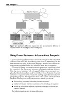
Figure 4.1 provides an example for three census tracts in Manhattan. Each
tract has a different proportion of the four characteristics being considered.
This data can be combined to get an overall fitness score for each tract. Note
that everyone in the tract gets the same score. The score represents the propor-
tion of the population in that tract that fits the profile.
470643 c04.qxd 3/8/04 11:10 AM Page 94
94 Chapter 4
the American population.
using two questionnaires, the short form and the long form (not counting
special purposes questionnaires, such as the one for military personnel). Most
the long form, which asks much more detailed questions about income,
these questionnaires provide the basis for demographic profiles.
most commonly used is the census tract, consisting of about 4,000 individuals.
population than other geographic units, such as counties and postal codes.
blocks and block groups;
Census Tract 189
Edu College+ 19.2%
Occ Prof+Exec 17.8%
HHI $75K+ 5.0%
HHI $100K+ 2.4%
Census Tract 122
Edu College+ 66.7%
Occ Prof+Exec 45.0%
HHI $75K+ 58.0%
HHI $100K+ 50.2%

Census Tract 129
Edu College+ 44.8%
Occ Prof+Exec 36.5%
HHI $75K+ 14.8%
HHI $100K+ 7.2%
DATA BY CENSUS TRACT
The U.S. government is constitutionally mandated to carry out an enumeration
of the population every 10 years. The primary purpose of the census is to
allocate seats in the House of Representatives to each state. In the process of
satisfying this mandate, the census also provides a wealth of information about
The U.S. Census Bureau (www.census.gov) surveys the American population
people get the short form, which asks a few basic questions about gender, age,
ethnicity, and household size. Approximately 2 percent of the population gets
occupation, commuting habits, spending patterns, and more. The responses to
The Census Bureau strives to keep this information up to date between each
decennial census. The Census Bureau does not release information about
individuals. Instead, it aggregates the information by small geographic areas. The
Although census tracts do vary in size, they are much more consistent in
The census does have smaller geographic units,
however, in order to protect the privacy of residents, some data is not made
available below the level of census tracts. From these units, it is possible to
aggregate information by county, state, metropolitan statistical area (MSA),
legislative districts, and so on. The following figure shows some census tracts in
the center of Manhattan:
470643 c04.qxd 3/8/04 11:10 AM Page 95
Data Mining Applications 95
(continued)
One philosophy of marketing is based on the old proverb “birds of a feather
already have customers and in similar areas. Census information can be
valuable, both for understanding where concentrations of customers are

DATA BY CENSUS TRACT
flock together.” That is, people with similar interests and tastes live in similar
areas (whether voluntarily or because of historical patterns of discrimination).
According to this philosophy, it is a good idea to market to people where you
located and for determining the profile of similar areas.
Goal Fitness
Edu College+ 19.2% 61.3% 0.31
17.8% 45.5% 0.39
HHI $75K+ 5.0% 22.6% 0.22
HHI $100K+ 2.4% 7.4% 0.32
0.31
Goal Fitness
Edu College+ 44.8% 61.3% 0.73
36.5% 45.5% 0.80
HHI $75K+ 14.8% 22.6% 0.65
HHI $100K+ 7.2% 7.4% 0.97
0.79
Goal Fitness
Edu College+ 66.7% 61.3% 1.00
45.0% 45.5% 0.99
HHI $75K+ 58.0% 22.6% 1.00
HHI $100K+ 50.2% 7.4% 1.00
1.00
Tract 189 Tract
Occ Prof+Exec
Overall Advertising Fitness
Tract 129 Tract
Occ Prof+Exec
Overall Advertising Fitness
Tract 122 Tract

Occ Prof+Exec
Overall Advertising Fitness
Figure 4.1 Example of calculating readership fitness for three census tracts in Manhattan.
Data Mining to Improve Direct
Marketing Campaigns
Advertising can be used to reach prospects about whom nothing is known as
individuals. Direct marketing requires at least a tiny bit of additional informa-
tion such as a name and address or a phone number or an email address.
Where there is more information, there are also more opportunities for data
mining. At the most basic level, data mining can be used to improve targeting
by selecting which people to contact.
470643 c04.qxd 3/8/04 11:10 AM Page 96
96 Chapter 4
Actually, the first level of targeting does not require data mining, only data.
In the United States, and to a lesser extent in many other countries, there is
quite a bit of data available about a large proportion of the population. In
many countries, there are companies that compile and sell household-level
data on all sorts of things including income, number of children, education
level, and even hobbies. Some of this data is collected from public records.
Home purchases, marriages, births, and deaths are matters of public record
that can be gathered from county courthouses and registries of deeds. Other
data is gathered from product registration forms. Some is imputed using mod-
els. The rules governing the use of this data for marketing purposes vary from
country to country. In some, data can be sold by address, but not by name. In
others data may be used only for certain approved purposes. In some coun-
tries, data may be used with few restrictions, but only a limited number of
households are covered. In the United States, some data, such as medical
records, is completely off limits. Some data, such as credit history, can only be
used for certain approved purposes. Much of the rest is unrestricted.
WARNING The United States is unusual in both the extent of commercially

available household data and the relatively few restrictions on its use. Although
household data is available in many countries, the rules governing its use differ.
There are especially strict rules governing transborder transfers of personal
data. Before planning to use houshold data for marketing, look into its
availability in your market and the legal restrictions on making use of it.
Household-level data can be used directly for a first rough cut at segmenta-
tion based on such things as income, car ownership, or presence of children.
The problem is that even after the obvious filters have been applied, the remain-
ing pool can be very large relative to the number of prospects likely to respond.
Thus, a principal application of data mining to prospects is targeting—finding
the prospects most likely to actually respond to an offer.
Response Modeling
Direct marketing campaigns typically have response rates measured in the
single digits. Response models are used to improve response rates by identify-
ing prospects who are more likely to respond to a direct solicitation. The most
useful response models provide an actual estimate of the likelihood of
response, but this is not a strict requirement. Any model that allows prospects
to be ranked by likelihood of response is sufficient. Given a ranked list, direct
marketers can increase the percentage of responders reached by campaigns by
mailing or calling people near the top of the list.
The following sections describe several ways that model scores can be
used to improve direct marketing. This discussion is independent of the data
470643 c04.qxd 3/8/04 11:10 AM Page 97
Data Mining Applications 97
mining techniques used to generate the scores. It is worth noting, however,
that many of the data mining techniques in this book can and have been
applied to response modeling.
According to the Direct Marketing Association, an industry group, a typical
mailing of 100,000 pieces costs about $100,000 dollars, although the price can
vary considerably depending on the complexity of the mailing. Of that, some

of the costs, such as developing the creative content, preparing the artwork,
and initial setup for printing, are independent of the size of the mailing. The
rest of the cost varies directly with the number of pieces mailed. Mailing lists
of known mail order responders or active magazine subscribers can be pur-
chased on a price per thousand names basis. Mail shop production costs and
postage are charged on a similar basis. The larger the mailing, the less impor-
tant the fixed costs become. For ease of calculation, the examples in this book
assume that it costs one dollar to reach one person with a direct mail cam-
paign. This is not an unreasonable estimate, although simple mailings cost less
and very fancy mailings cost more.
Optimizing Response for a Fixed Budget
The simplest way to make use of model scores is to use them to assign ranks.
Once prospects have been ranked by a propensity-to-respond score, the
prospect list can be sorted so that those most likely to respond are at the top of
the list and those least likely to respond are at the bottom. Many modeling
techniques can be used to generate response scores including regression mod-
els, decision trees, and neural networks.
Sorting a list makes sense whenever there is neither time nor budget to
reach all prospects. If some people must be left out, it makes sense to leave out
the ones who are least likely to respond. Not all businesses feel the need to
leave out prospects. A local cable company may consider every household in
its town to be a prospect and it may have the capacity to write or call every one
of those households several times a year. When the marketing plan calls for
making identical offers to every prospect, there is not much need for response
modeling! However, data mining may still be useful for selecting the proper
messages and to predict how prospects are likely to behave as customers.
A more likely scenario is that the marketing budget does not allow the same
level of engagement with every prospect. Consider a company with 1 million
names on its prospect list and $300,000 to spend on a marketing campaign that
has a cost of one dollar per contact. This company, which we call the Simplify-

ing Assumptions Corporation (or SAC for short), can maximize the number of
responses it gets for its $300,000 expenditure by scoring the prospect list with
a response model and sending its offer to the prospects with the top 300,000
scores. The effect of this action is illustrated in Figure 4.2.
470643 c04.qxd 3/8/04 11:10 AM Page 98
98 Chapter 4
ROC CURVES
Models are used to produce scores. When a cutoff score is used to decide
which customers to include in a campaign, the customers are, in effect, being
classified into two groups—those likely to respond, and those not likely to
respond. One way of evaluating a classification rule is to examine its error
rates. In a binary classification task, the overall misclassification rate has two
components, the false positive rate, and the false negative rate. Changing the
cutoff score changes the proportion of the two types of error. For a response
model where a higher score indicates a higher liklihood to respond, choosing a
high score as the cutoff means fewer false positive (people labled as
responders who do not respond) and more false negatives (people labled as
nonresponders who would respond).
An ROC curve is used to represent the relationship of the false-positive rate
to the false-negative rate of a test as the cutoff score varies. The letters ROC
stand for “Receiver Operating Characteristics” a name that goes back to the
curve’s origins in World War II when it was developed to assess the ability of
radar operators to identify correctly a blip on the radar screen , whether the
blip was an enemy ship or something harmless. Today, ROC curves are more
likely to used by medical researchers to evaluate medical tests. The false
positive rate is plotted on the X-axis and one minus the false negative rate is
plotted on the Y-axis. The ROC curve in the following figure
ROC Chart
100
90

80
70
60
50
40
30
20
10
0
0 20 40 60 80 100