Algorithms and Networking for Computer Games phần 2 pptx
Bạn đang xem bản rút gọn của tài liệu. Xem và tải ngay bản đầy đủ của tài liệu tại đây (313.23 KB, 29 trang )
INTRODUCTION 5
The Controller part includes the components for the participation role. Control logic
affects the Model and keeps up the integrity (e.g. by excluding illegal moves suggested
by a player). The human player’s input is received through an input device filtered by
a driver software. The configuration component provides instance data, which is used in
generating the initial state for the game. The human player participates in the data flow by
perceiving information from the output devices and performing actions through the input
devices. Although the illustration in Figure 1.2 includes only one player, naturally there
can be multiple players participating the data flow, each with thier own output and input
devices. Moreover, the computer game can be distributed among several nodes rather than
reside inside a single node. Conceptually, this is not a problem since the components in the
MVC can as well be thought to be distributed (i.e. the data flows run through the network
rather than inside a single computer). In practice, however, the networked computer games
provide their own challenges (see Section 1.3).
1.2 Synthetic Players
A synthetic player is a computer-generated actor in the game. It can be an opponent, a
non-player character (NPC) that participates limitedly (like a supporting actor), or a deus
ex machina, which can control natural forces or godly powers and thus intervene or generate
thegameevents.
Because everything in a computer game revolves around the human player, the game
world is anthropocentric. Regardless of the underlying method for decision-making (see
Chapter 6), the synthetic player is bound to show certain behaviour in relation to the
human player, which can range from simple reactions to general attitudes and even complex
intentions. As we can see in Figure 1.2, the data flow of the human player and the synthetic
player resemble each other, which allows us to project human-like features to the synthetic
player.
We can argue that, in a sense, there should be no difference between the players whether
they are humans or computer programs; if they are to operate on the same level, both
should ideally have the same powers of observation and the same capabilities to cope
with uncertainties (see Chapter 7). Ideally, the synthetic players should be in a similar
situation as their human counterparts, but of course a computer program is no match for
human ingenuity. This is why synthetic players rarely display real autonomy but appear to
behave purposefully (e.g. in Grand Theft Auto III pedestrians walk around without any real
destination).
The more open (i.e. the less restrictive) the game world is, the more complex the
synthetic players are. This trade-off between the Model and the Controller software com-
ponents is obvious: If we remove restricting code from the core structures, we have to
reinstate it in the synthetic players. For example, if the players can hurt themselves by
walking into fire, the synthetic player must know how to avoid it. Conversely, if we rule
out fire as a permitted area, path finding (see Chapter 5) for a synthetic player becomes
simpler.
Let us take a look at two external features that a casual player is most likely to notice
first in a synthetic player: humanness and stance. They are also relevant to the design of
the synthetic player by providing a framework for the game developers and programmers.
6 INTRODUCTION
1.2.1 Humanness
The success of networked multi-player games can be, at least in part, explained with
the fact that the human players provide something that the synthetic ones still lack. This
missing factor is the human traits and characteristics – flaws as much as (or even more
than) strengths: fear, rage, compassion, hesitation, and emotions in general. Even minor
displays of emotion can make the synthetic player appear more human. For instance, in
Half-Life and Halo the synthetic players who have been taken by surprise do not act in
superhuman coolness but show fear and panic appropriate to the situation. We, as human
beings, are quite apt to read humanness into the decisions even when there is nothing but
na
¨
ıve algorithms behind them. Sometimes a game, such as NetHack , even gathers around
a community that starts to tell stories of the things that synthetic players have done and to
interpret them in human terms.
A computer game comprising just synthetic players could be as interesting to watch as
a movie or a television show (Charles et al. 2002). In other words, if the game world is
fascinating enough to observe, it is likely that it is also enjoyable to participate in – which
is one of the key factors in games like The Sims and Singles, where the synthetic players
seem to act (more or less) with a purpose and the human player’s influence is, at best, only
indirect.
There are also computer games that do not have human players at all. In the 1980s
Core War demonstrated that programming synthetic players to compete with each other
can be an interesting game by itself (Dewdney 1984). Since then some games have tried to
use this approach, but, by and large, artificial intelligence (AI) programming games have
only been the by-products of ‘proper’ games. For example, Age of Empires II includes a
possibility to create scripts for computer players, which allows to organize games where
programmers compete on who creates the best AI script. The whole game is then carried
out by a computer while the humans remain as observers. Although the programmers
cannot affect the outcome during the game, they are more than just enthusiastic watchers:
They are the coaches and the parents, and the synthetic players are the prot
`
eg
`
es and the
children.
1.2.2 Stance
The computer-controlled player can have different stances (or attitudes) towards the human
player. Traditionally, the synthetic player has been seen only in the role of an enemy. As
an enemy, the synthetic player must provide challenge and demonstrate intelligent (or at
least purposeful) behaviour. Although the enemies may be omniscient or cheat when the
human player cannot see them, it is important to keep the illusion that the synthetic player
is at the same level as the human player.
When the computer acts as an ally, its behaviour must adjust to the human point of view.
For example, a computer-controlled reconnaissance officer should provide intelligence in a
visually accessible format rather than overwhelm the player with lists of raw variable values.
In addition to accessibility, the human players require consistency, and even incomplete
information (as long as it remains consistent) can have some value to them. The help can
even be concrete operations like in Neverwinter Nights or Star Wars: Battlefront where the
computer-controlled teammates respond to the player’s commands.
INTRODUCTION 7
The computer has a neutral stance when it acts as an observer (e.g. camera director or
commentator) or a referee (e.g. judging rule violations in a sports game) (Siira 2004). Here,
the behaviour depends on the context and conventions of the role. In a sports game, for
example, the camera director program must heed the camera placements and cuts dictated by
the television programme practice. Refereeing provides another kind of challenge, because
some rules can be hard to judge. Finally, synthetic players can be used to carry on the plot,
to provide atmosphere, or simply to act as extras. Nevertheless, as we shall see next, they
may have an important role in assisting immersion in the game world and directing the
game play.
1.3 Multi-playing
What keeps us interested is – surprise. Humans are extremely creative at this, whereas
a synthetic player can be lacking in humaneness. One easy way to limit the resources
dedicated to the development of synthetic players is to make the computer game a multi-
player game.
The first real-time multi-player games usually limited the number of players to two,
because the players had to share the same computer by dividing either the screen (e.g.
Pitstop II ) or the playtime among the participating players (e.g. Formula One Grand Prix).
Also, the first networked real-time games connected two players over a modem (e.g. Falcon
A.T.). Although text-based networked multi-player games started out in the early 1980s with
Multi-user dungeons (MUDs) (Bartle 1990), real-time multi-player games (e.g. Quake)
became common in the 1990s as local area networks (LANs) and the Internet became
more widespread. These two development lines were connected when online game sites
(e.g. Ultima Online) started to provide real-time multi-player games for a large number of
players sharing the same game world.
On the technical level, networking in multi-player computer games depends on achieving
a balance between the consistency and responsiveness of a distributed game world (see
Chapter 9). The problems are due to the inherent technical limitations (see Chapter 8). As
the number of simultaneous players increases, scalability of the chosen network architecture
becomes critical. Although related research work on interactive real-time networking has
been done in military simulations and networked virtual environments (Smed et al. 2002,
2003), cheating prevention is a unique problem for computer games (see Chapter 10).
Nowadays, commercially available computer games are expected to offer a multi-player
option, and, at the same time, online game sites are expected to support an ever increasing
number of users. Similarly, the new game console releases rely heavily on the appeal of
online gaming, and a whole new branch of mobile entertainment has emerged with intention
to develop distributed multi-player games for wireless applications.
The possibility of having multiple players enriches the game experience – and compli-
cates the software design process – because of the interaction between the players, both
synthetic and human. Moreover, the players do not have to be opponents but they can co-
operate. Although more common in single-player computer games, it is possible to include
a story-like plot in a multi-player game, where the players are cooperatively solving the
story (e.g. No One Lives Forever 2 and Neverwinter Nights). Let us next look at storytelling
from a broader perspective.
8 INTRODUCTION
1.4 Games and Storytelling
Storytelling is about not actions but reasons for actions. Human beings use stories to
understand intentional behaviour and tend to ‘humanize’ the behaviour of the characters to
understand the story (Spierling 2002). While ‘traditional’ storytelling progresses linearly,
a game must provide an illusion of free will (Costikyan 2002). According to Aylett and
Louchart (2003), computer games differ from other forms of storytelling in that the story
time and real time are highly contingent, whereas in traditional forms of storytelling (e.g.
cinema or literature) this dependency can be quite loose. Another differentiating factor
is interactivity, which is non-existent or rather restricted in other forms of storytelling.
Bringsjord (2001) lists four challenges to interactive storytelling: First, a plot and three-
dimensional characters are not enough to produce a high-quality narrative but there has
to be a theme (e.g. betrayal, self-deception, love, or revenge) behind them. Second, there
should exist some element to make the story stay dramatically interesting. Third, apart from
being robust and autonomous, the characters (i.e. synthetic players) have to be memorable
personalities by themselves. Fourth, a character should understand the players – even to
the point of inferring other characters’ and players’ beliefs on the basis of its own beliefs.
Anthropocentrism is reflected not only in the reactions but also in the intentions of
the synthetic players. As a form of entertainment, amusement, or pastime, the intention of
games is to immerse and engulf the human player fully in the game world. This means that
the human player may need guidance while proceeding with the game. The goals of the
game can get blurry, and synthetic players or events should lead the human players so that
they do not stray too far from the intended direction set by the developers of the game. For
this reason, the game developers are quite eager to include a story into the game. The usual
approach to include storytelling into commercial computer games is to have ‘interactive
plots’ (International Game Developers Association 2004). A game may offer only a little
room for the story to deviate – like in Dragon’s Lair, where, at each stage, the players
can choose from several alternative actions of which all but one leads to a certain death.
This linear plot approach is nowadays replaced by the parallel paths approach, where the
story line is divided into episodes. The player has some freedom within the episode, which
has fixed entry and exit points. At the transition point, the story of the previous episode
is concluded and new story alternatives for the next episode are introduced. For instance,
in Max Payne or Diablo II , the plot lines of the previous chapter are concluded at the
transition point, and many new plot alternatives are introduced. Still, many games neither
include a storyline nor impose a sequence of events. Granted that some of them can be
tedious (e.g. Frontier: Elite II , in which the universe is vast and devoid of action whereas
in the original Elite the goal remains clearer) – but so are many games that include a story.
Research on storytelling computer systems is mainly motivated by the theories of
V. Propp (1968), because they help to reduce the task of storytelling to a pattern recognition
problem; for example, see Fairclough and Cunningham (2002); Lindley and Eladhari (2002);
Peinado and Gerv
´
as (2004). This pattern recognition approach can even be applied hier-
archically to different abstraction levels. Spierling et al. (2002) decompose the storytelling
system into four parts: story engine, scene action engine, character conversation engine, and
actor avatar engine. These engines either rely on pre-defined data or act autonomously, and
the higher level sets the outline for the level below. For example, on the basis of the cur-
rent situation the story engine recognizes an adaptable story pattern and inputs instructions
INTRODUCTION 9
for the scene action engine to carry out. In addition to these implementation-oriented ap-
proaches, other methodological approaches to interactive storytelling have been suggested
in the fields of narratology and ludology, but we omit a detailed discussion of them here.
The main problem with the often-used top-down approach is that the program generating
the story must act like a human dungeon master. It must observe the reactions of the crowd
as well as the situation in the game, and recognize what pattern fits the current situation:
Is the game getting boring and should there be a surprising twist in the plot, or has there
been too much action and the players would like to have a moment’s peace to rest and
regroup? Since we aim at telling a story to the human players, we must ensure that the world
around them remains purposeful. We have general plot patterns that we try to recognize
in the history and in the surroundings of a human player. This in turn determines how the
synthetic players will act.
Instead of a centralized and omnipotent storyteller or dominant dungeon master, the plot
could get revealed and the (autobiographical) ‘story’ of the game (as told by the players
to themselves) could emerge from the interaction with the synthetic players. However, this
bottom-up approach is, quite understandably, rarely used because it leaves the synthetic
players alone with a grave responsibility: They must provide a sense of purpose in the
chaotic world.
1.5 Other Game Design Considerations
Although defining what makes a game enjoyable is subjective, we can list some features
that alluring computer games seem to have. Of course, our list is far from complete and
open to debate, but we want to raise certain issues that are interesting in their own right
but which – unfortunately – fall out of the scope of this book.
• Customization: A good game has an intuitive interface that is easy to learn. Because
players have their own preferences, they should be allowed to customize the user
interface to their own liking. For example, the interface should adapt dynamically
to the needs of a player so that in critical situations the player has more detailed
control. If a player can personalize her avatar (e.g. customize the characteristics to
correspond to her real-world persona), it can increase the immersion of the game.
• Tutorial : The first problem a player faces is learning how the game works, which
includes both the user interface and the game world. Tutorials are a convenient method
for teaching the game mechanics to the player, where the player can learn the game
by playing it in an easier and possibly assisted mode.
• Profiles: To keep the game challenging as the player progresses, it should support
different difficulty levels that provide new challenges. Typically, this feature is imple-
mented by increasing certain attributes of the enemies: their number, their accuracy,
and their speed. The profile can also include the player’s preferences of the type of
game (e.g. whether it should focus on action or adventure).
• Modifications: Games gather communities around them, and members of the com-
munity start providing new modifications (or ‘mods’) and add-ons to the original
game. A modification can be just a graphical enhancement (e.g. new textures) or it
10 INTRODUCTION
can enlarge the game world (e.g. new levels). Also, the original game developers
themselves can provide extension packs, which usually include new levels, playing
characters, and objects, and perhaps some improvement of the user interface.
• Replaying: Once is not enough. We take pictures and videotape our lives. The same
also applies to games. Traditionally, many games provide the option to take screen
captures, but replays are also an important feature. Replaying can be extended to
cover the whole game, and the recordings allow the players to relive and memorize
the highlights of the game, and to share them with friends and the whole game
community.
It is important to recognize beforehand what software development mechanisms are pub-
lished to the players and with what interfaces. The game developers typically implement
special software for creating content for the game. These editing tools are a valuable surplus
to the final product. If the game community can create new variations of the original game,
longevity of the game increases. Furthermore, the inclusion of the developing tools is an
inexpensive way – since they are already implemented – to enrich the contents of the final
product.
Let us turn the discussion around and ask what factors are responsible for making a
computer game bad. It can be summed in one word: limitation. Of course, to some extent
limitation is necessary – we are, after all, dealing with limited resources. Moreover, the
rules of the game are all about limitation, although their main function is to impose the
goals for the game. The art of making games is to balance the means and limitations so
that this equilibrium engrosses the human player. How do limitations manifest themselves
in the program code? The answer is the lack of parameters: The more the things are hard-
coded, the lesser the possibilities to add and support new features. Rather than shutting
out possibilities, a good game – like any good computer program! – should be open and
modifiable for both the developer and the player.
1.6 Outline of the Book
The intention of our book is to look at the algorithmic and networking problems present in
commercial computer games from the perspective of a computer scientist. As the title im-
plies, this book is divided into two parts: algorithms and networking. This emphasis on topic
selection leaves out components of Figure 1.2 that are connected to the human-in-the-loop.
Most noticeably, we omit all topics concerning graphics and human interaction – which
is not to say that they are in any way less important or less interesting than the current
selection of topics. Also, game design as well as ludological aspects of computer games
fall out of the scope of this book.
The topics of the book are based on the usual problems that game developers encounter
in game programming. We review the theoretical background of each problem and review
the existing methods for solving them. The given algorithmic solutions are given not in any
specific programming language but in pseudo-code format, which can be easily rewritten
in any programming language and – more importantly – which emphasizes the algorithmic
idea behind the solution. The algorithmic notation used is described in detail in Appendix A.
INTRODUCTION 11
We have also included examples from real-world computer games to clarify different
uses for the theoretical methods. In addition, each chapter is followed by a set of exercises,
which go over the main points of the chapter and extend the topics by introducing new
perspectives.
1.6.1 Algorithms
Part I of this book concentrates on typical algorithmic problems in computer games and
presents solution methods. The chapters address the following questions:
• Chapter 2 – Random Numbers: How can we achieve indeterminism required by
games using deterministic algorithms?
• Chapter 3 – Tournaments: How we can form a tournament to decide a ranking for a
set of contestants?
• Chapter 4 – Game Trees: How can we build a synthetic player for perfect information
games?
• Chapter 5 – Path Finding: How can we find a route in a (possibly continuous) game
world?
• Chapter 6 – Decision-Making: How can we make a synthetic player act intelligently
in the game world?
• Chapter 7 – Modelling Uncertainty: How can we model the uncertainties present in
decision-making?
1.6.2 Networking
Part II turns the attention to networking. We aim at describing the ideas behind different
approaches rather than get too entangled in the technical details. The chapters address the
following questions:
• Chapter 8 – Communication Layers: What are the technical limitations behind net-
working?
• Chapter 9 – Compensating Resource Limitations: How can we cope with the inherent
communication delays and divide the network resources among multiple players?
• Chapter 10 – Cheating Prevention: Can we guarantee a fair playing field for all play-
ers?
1.7 Summary
All games have a common basic structure comprising players, rules, goals, opponents, and
representation. They form the challenge, play, and conflict aspects of a game, which are
reflected, for instance, in the Model–View–Controller software architecture pattern. The
computer can participate in the game as a synthetic player, which can act in the role of
12 INTRODUCTION
an opponent or a teammate or have a neutral stance. For example, synthetic player must
take the role of a storyteller, if we want to incorporate story-like features into the game.
Multi-playing allows other human players to participate in the same game using networked
computers.
Game programming has matured from its humble beginnings and nowadays it resembles
any other software project. Widely accepted software construction practices have been
adopted in game development, and, at the same time, off-the-shelf components (e.g. 3D
engines and animation tools) have removed the burden to develop all software components
in house. This maturity, however, does not mean that there is no room for artistic creativity
and technical innovations. There must be channels for bringing out novel and possibly
radically different games, and, like music and film industry, independent game publishing
can act as a counterbalance to the mainstream.
Nevertheless computer games are driven by computer programs propelled by algorithms
and networking. Let us see what they have in store for us.
Exercises
1-1 Take any simple computer game (e.g. Pac-Man) and discern what forms its challenge
aspect (i.e. player, rules and goal), conflict aspect, and play aspect.
1-2 A crossword puzzle is not a game (or is it?). What can you do to make it more
game-like?
1-3 Why do we need a proto-view component in the MVC decomposition?
1-4 What kind of special skills and knowledge should game programmers have when they
are programming
(a) the Model part software components,
(b) the View part software components, or
(c) the Controller part software components?
1-5 Let us look at a first-person shooter (FPS) game (e.g. Doom or Quake). Discern the
required software components by using the MVC. What kind of modelling does it
require? What kind of View-specific considerations should be observed? How about
the Controller part?
1-6 Deus ex machina (from Latin ‘god from the machine’) derives from ancient theater,
where the effect of the god’s appearance in the sky, to solve a crisis by divine
intervention, was achieved by means of a crane. If a synthetic player participates in
thegameasadeus ex machina, what kind of role will it have?
1-7 What does ‘anthropocentrism’ mean? Are there non-anthropocentric games?
1-8 The Sims includes an option of free will. By turning it off, the synthetic players do
nothing unless the player explicitly issues a command. Otherwise, they show their
own initiative and follow, for example, their urges and needs. How much free will
INTRODUCTION 13
should a synthetic player have? Where would it serve the best (e.g. in choosing a
path or choosing an action)?
1-9 Many games are variations of the same structure. Consider Pac-Man and Snake.
Discern their common features and design a generic game that can be parameterized
to be both the games.
1-10 Judging rules can be difficult – even for an objective computer program. In football (or
soccer as some people call it), the official rules say that the referee can allow the play
to continue ‘when the team against which an offence has been committed will benefit
from such an advantage’ and penalize ‘the original offence if the anticipated advantage
does not ensue at that time’ (Federation Internationale de Football Association 2003).
How would you implement this rule? What difficulties are involved in it?
Part I
Algorithms
2
Random Numbers
One of the most difficult problems in computer science is implementing a truly random
number generator – even D.E. Knuth devotes a whole chapter of his book The Art of Com-
puter Programming to the topic (Knuth 1998b, Chapter 3). The difficulty stems partly from
how we understand the word ‘random’, since no single number in itself is random. Hence,
the task is not to simulate randomness but to generate a virtually infinite sequence of sta-
tistically independent random numbers uniformly distributed inside a given interval (Park
and Miller 1988).
Because algorithms are deterministic, they cannot generate truly random numbers –
except with the help of some outside device like processor-embedded circuits (Intel Platform
Security Division 1999). Rather, the numbers are generated with arithmetic operations, and,
therefore, the sequences are not random but appear to be so – hence, they are often said to
be pseudo-random. It is quite easy to come up with methods like von Neumann’s middle-
square method, where we take the square of the previous random number and extract
the middle digits; for example, if we are generating four-digit numbers, the sequence can
include a subsequence:
r
i
= 8269
r
i+1
= 3763 (r
2
i
= 68376361)
r
i+2
= 1601 (r
2
i+1
= 14160169)
.
.
.
However, if we analyse this method more carefully, it will soon become clear why it is
hardly satisfactory for the current purpose. This holds also for many other ad hoc methods,
and Knuth sums up his own toils on the subject by exclaiming that ‘random numbers should
not be generated with a method chosen at random’ (Knuth 1998b, p. 6).
Since every random number generator based on arithmetic operations has its inbuilt
characteristic regularities, we cannot guarantee it will work everywhere. This problem is
due to the fact that the pseudo-random number sequence produced is fixed and devised
separately from the contexts of its actual use. Still, empirical testing and application-specific
analysis can provide safety measures against deficiencies (Hellekalek 1998). The goal is
Algorithms and Networking for Computer Games Jouni Smed and Harri Hakonen
2006 John Wiley & Sons, Ltd
18 RANDOM NUMBERS
to find such methods that produce sequences that are unlikely to get ‘synchronized’ to
their contexts. Other aspects that may affect the design of random number generators are
the speed of the algorithm, ease of implementation, parallelization, and portability across
platforms.
Before submerging in the wonderful world of pseudo-random numbers, let us take a
small sidetrack and acknowledge that sometimes we can do quite well without randomness.
Most people hardly consider the sequence S =0, 1, 2, 3, 4, 5, 6, 7 random, because it is
easy to come up with a rule that generates it: S
i+1
= (S
i
+ 1) mod m. But how about the
sequence R =0, 4, 2, 6, 1, 5, 3, 7? There seems to be no direct relationship between two
consecutive values, but as a whole the sequence has a structure: even numbers precede
odd numbers. A bit-aware reader may soon realize that R
i
= Bit-Reverse(i, 3) is a simple
model that explains R. Then, how about the sequence Q =0, 1, 3, 2, 6, 7, 5, 4? It seems to
have no general structure, but the difference between consecutive pairs is always one, which
is typical for a binary-reflected Gray code. From these simple examples, we can see that
sequences can have properties that are useful in certain contexts. If these characteristics are
not used or observed – or not even discovered! – the sequence can appear to be random.
To make a distinction, these random-like (or ‘randomish’) numbers are usually called quasi-
random numbers. Quasi-randomness can be preferable to pseudo-randomness, for example,
when we want to have a sequence that has a certain inherent behaviour or when we can
calculate the bijection of a value and its index in the sequence.
2.1 Linear Congruential Method
At the turn of the 1950s, D.H. Lehmer proposed an algorithm for generating random num-
bers. This algorithm is known as the linear congruential method, and since its inception
it has stood the test of time quite firmly. The algorithm is simple to implement and only
requires a rigorous choice of four fixed integer parameters:
modulus: m(0 <m)
multiplier: a(0 ≤ a<m)
increment: c(0 ≤ c<m)
starting value: X
0
(0 ≤ X
0
<m)
On the basis of these parameters, we can now obtain a sequence of random numbers by
setting
X
i+1
= (aX
i
+ c) mod m(0 ≤ i). (2.1)
This recurrence produces a repeating sequence of numbers denoted by X
i
i≥0
.Moregen-
erally, let us define
b = a −1
and assume that
a ≥ 2,b≥ 1.
We can now generalize Equation (2.1) to
X
i+k
= (a
k
X
i
+ (a
k
− 1)c/b) mod m(k≥ 0,i≥ 0), (2.2)
which expresses the (i +k)th term directly in terms of the ith term.
RANDOM NUMBERS 19
Algorithm 2.1 describes two implementation variants of the linear congruential method
defined by Equation (2.1). The first one can be used when a(m − 1) does not exceed the
largest integer that can be represented by the machine word. For example, if m is a one-word
integer, the product a(m −1) must be evaluated within a two-word integer. The second
variant can be applied when (m mod a) ≤m/a. The idea is to express the modulus in
the form m = aq + p to guarantee that the intermediate evaluations always stay within
the interval (−m, m). For a further discussion on implementation, see Wichmann and Hill
(1982), L’Ecuyer (1988), Park and Miller (1988), L’Ecuyer and C
ˆ
ot
´
e (1991), Bratley et al.
(1983, pp. 201–202), and Knuth (1998b, Exercises 3.2.1.1-9 and 3.2.1.1-10).
Because computer numbers have a finite accuracy, m is usually set close to the maximum
value of the computer’s integer number range. If we want to generate random floating point
numbers where U
i
is distributed between zero (inclusive) and one (exclusive), we can use
the fraction U
i
= X
i
/m instead and call this routine Random-Unit().
What if we want a random integer number within a given interval of length w (0 <
w ≤ m)? A straightforward solution would be to use the Monte Carlo approach and let
Y
i
= X
i
mod w or – to put it in another way – to let Y
i
=U
i
w. However, the problem
with this method is that the distribution is not guaranteed to be uniform (see Figure 2.1),
but Monte Carlo methods allow to reduce the approximateness of the solution at the cost of
the running time. In this case, we could increase the range of the original random number,
for example, by generating several random numbers and combining them, which would
make the distribution more uniform but would require more computation.
The Las Vegas approach guarantees exactness and gives a simple solution, a uniform
distribution, to our problem. This method partitions the original interval
[0,m− 1] =
w−1
i=0
i
m
w
,(i+1)
m
w
− 1
∪
w
m
w
,m− 1
,
where i gives the value in the new interval (0 ≤ i ≤ w − 1). The last interval (if existing) is
excess and considered invalid (see Figure 2.2). Algorithm 2.2 implements this partitioning
by using integer division. If a generated number falls within the excess range, a new
one is generated until it is valid. The obvious downside is that the termination of the
algorithm is not guaranteed. Nevertheless, if we consider the worst case where w =
m
2
+ 1,
the probability of not finding a solution after i rounds is of magnitude 1/2
i
.
9012345678
= 4
m = 10
321
0
w
Figure 2.1 If m = 10 and w = 4, the Monte Carlo method does not provide a uniform
distribution.
20 RANDOM NUMBERS
Algorithm 2.1 Linear congruential method for generating random integer numbers within
the interval [0,m).
Random()
out: random integer r (0 ≤ r ≤ m −1)
constant: modulus m; multiplier a; increment c; starting value X
0
(1 ≤ m ∧ 0 ≤
a, c, X
0
≤ m −1 ∧a ≤ i
max
/(m − 1),wherei
max
is the largest possible in-
teger value)
local: previously generated random number x (initially x = X
0
)
1: r ← (a ·x) mod m
2: r ← Modulo-Sum(r, c, m)
3: x ← r
4: return r
Random()
out: random integer r (0 ≤ r ≤ m −1)
constant: modulus m; multiplier a; increment c; starting value X
0
(1 ≤ m ∧ 0 ≤
a, c, X
0
≤ m −1 ∧(m mod a) ≤m/a)
local: previously generated random number x (initially x = X
0
)
1: q ← m div a
2: p ← m mod a
3: r ← a ·(x mod q) − p · (x div q)
4: if r<0 then
5: r ← r + m
6: end if
7: r ← Modulo-Sum(r, c, m)
8: x ← r
9: return r
Modulo-Sum(x,y,m)
in: addends x and y; modulo m (0 ≤ x,y ≤ m − 1)
out: value (x +y) mod m without intermediate overflows in [0,m− 1]
1: if x ≤ m − 1 −y then
2: return x +y
3: else
4: return x −(m −y)
5: end if
2.1.1 Choice of parameters
Although the linear congruential method is simple to implement, the tricky part is choosing
values for the four parameters. Let us have a look at how they should be chosen and how
we can analyse their effect.
The linear congruential method generates a finite sequence of random numbers, after
which the sequence begins to repeat. For example, if m = 12 and X
0
= a = c = 5, we get
RANDOM NUMBERS 21
Excess
w
m = 10
12 345 678 9
0312
= 4
0
Figure 2.2 The Las Vegas method distributes the original interval uniformly by defining
the excess area as invalid.
Algorithm 2.2 Las Vegas method for generating random integer numbers within the interval
[, u).
Random-Integer(, u)
in: lower bound (0 ≤ ); upper bound u(<u≤ + m)
out: random integer r ( ≤ r ≤ u)
constant: modulus m used in Random()
local: the largest value w in the subinterval [0,u− ] ⊆ [0,m− 1]
1: w ← u −
2: repeat
3: r ← Random() div (m div w)
4: until r < w
5: r ← r +
6: return r
the sequence
6, 11, 0, 5, 6, 11, 0, 5,
The repeating cycle is called a period, and, obviously, we want it to be as long as possible.
Note that the values in the period of the linear congruential method are different, and
it is impossible to have repetitions – unless we, for example, re-scale the interval with
Random-Integer(, u) or combine multiple sequences into one (Wichmann and Hill 1982).
However, a long period does not guarantee randomness: The longest period of length m
can always be reached by letting a = c = 1 (but you can hardly call the generated sequence
random). Luckily, there are other values that reach the longest period, as the Theorem 2.1.1
shows.
Theorem 2.1.1 The linear congruential sequence defined by integer parameters m, a, c,
and X
0
has period length m if and only if
(i) the greatest common divisor for c and m is 1,
(ii) b is a multiple of each prime dividing m, and
(iii) if m is a multiple of 4, then b is also a multiple of 4.
We have denoted b = a −1. For a proof, see (Knuth 1998b, pp. 17–19).
22 RANDOM NUMBERS
Modulus
Since the period cannot have more than m elements, the value of m should be large. Ideally
m should be i
max
+ 1, where i
max
is the maximum value of the integer value range. For
example, if the machine word is unsigned and has 32 bits, we let m = (2
32
− 1) + 1 = 2
32
.
In this case, the computation can eliminate the modulo operation completely. Similarly, if m
is a power of two, the modulo operation can be replaced by a quicker bitwise-and operation.
Unfortunately, these m values do not necessarily provide us with good sequences, not even
if Theorem 2.1.1 holds.
Primes or Mersenne primes are much better choices for the value of m. A Mersenne
prime is a prime of the form of 2
n
− 1; the first 10 Mersenne primes have n = 2, 3, 5, 7,
13, 17, 19, 31, 61, and 89 respectively. Quite conveniently, 2
31
− 1 is a Mersenne prime
and thus it is often used with 32-bit machine words.
Multiplier
The multiplier a should be chosen so as to produce a period of maximum length. From
Theorem 2.1.1 it follows that if m is the product of distinct primes, only when a = 1we
will get a full period. However, if m is divisible by a high power of some prime, we have
more choices for a. There is a fundamental problem with small a values: If X
i
is small,
it is probable that X
i+1
is also small. As a rule of thumb, the multiplier a should reside
between 0.01 and 0.99m, and its binary representation should not have a simple, regular bit
pattern. For example, multipliers of the form a = 2
x
+ 1(2≤ x) have a regular bit pattern
and, therefore, tend to produce low-quality random sequences.
Increment
From Theorem 2.1.1 it also follows that the increment c can be chosen quite freely as long
as it does not have a common factor with m (e.g. c = 1orc = a). In many implementations
c = 0, because it allows the elimination of one operation and makes the processing a bit
faster. However, as Theorem 2.1.1 indicates, this cuts down the length of the period. Also,
when c = 0, we must guarantee that X
0
= 0.
Starting value
The starting value (or seed) X
0
determines from where in the sequence the numbers are
taken. A common oversight in the initialization is to always use the same seed value,
because it leads to the same sequence of generated numbers. Usually this can be avoided
by obtaining the seed value from the built-in clock of the computer, the last value from
the previous run, user’s mouse movements, previously handled keystrokes, or some other
varying source.
2.1.2 Testing the randomness
Random number generators can be tested both empirically and theoretically. We omit the
theoretical discussion and go through some rudiments of empirical tests; curious readers
are referred to Knuth (1998b, Section 3.3). In most cases, the following tests are based
on statistical tests (e.g. χ
2
or Kolmogorov–Smirnov) and they aim at providing some
RANDOM NUMBERS 23
quantitative measures for randomness, when choosing between different parameter settings.
Nevertheless, one should bear in mind that, although a random sequence might behave well
in an existing test, there is no guarantee that it will pass a further test; each test gives us
more confidence but can never banish our doubts.
Frequency test Are numbers distributed uniformly according to their frequencies?
Serial test Are pairs (triplets, quadruplets etc.) of successive numbers uniformly distributed
in an independent manner?
Gap test Given a range of numbers, what is the distribution of the gaps between their
occurrences in the sequence?
Poker test Group the sequence into poker hands each comprising five consecutive integers.
Are the hands distributed as random poker hands should be?
Coupon collector’s test What is the length of sequence required to get a complete set of
given integers?
Permutation test Divide the sequence into groups of a given size. How often do different
permutations occur?
Run test How long are the monotone segments (run-ups or run-downs of consecutive num-
bers) of the sequence?
Collision test If numbers are categorized with a hash function, how many collisions would
occur?
Birthday spacings test If the numbers are hashed, how long are the spacings between them?
Spectral test If pairs (triplets, quadruples etc.) of successive numbers are treated as points
in a hypercube, how uniformly would they fill it?
Spectral test is an important (and yet quite intuitive) test for analysing linear congruential
random number generators. Moreover, we can rest assured that all good generators will
pass the test and bad ones are likely to fail it. Although it is an empirical test and requires
computation, it resembles theoretical tests in the sense that it deals with the properties of
the full period.
Suppose we have a sequence of period m and we take t consecutive numbers of the
sequence so that we have a set of points
{(X
i
,X
i+1
, ,X
i+t−1
) | 0 ≤ i<m}
in t-dimensional space. For example, if t = 2, we can draw the points in a two-dimensional
plane (see Figure 2.3). In this case, one can easily discern the parallel lines into which
the points fall. This is an inherent property of the linear congruential methods: When t
increases, the periodic accuracy decreases as there are fewer hyperplanes where the points
can reside. In contrast, a truly random sequence would have the same accuracy in all
dimensions.
24 RANDOM NUMBERS
Figure 2.3 Two-dimensional spectral test results for the case where m = 256, a = 21, and
c = 11.
2.1.3 Using the generators
Although the programmer implementing a random number generator must understand the
theory behind the method, the user also has responsibilities. If one does not know the
assumptions behind the linear congruential method, it can easily become a random number
‘degenerator’. To prevent this from happening, let us go through some common pitfalls
lurking in pseudo-random numbers generated by Equation (2.1).
• If X
0
= 0, the largest range of multiplicative linear congruential method X
i+1
=
aX
i
mod m is [1,m− 1]. However, the range of U
i
= X
i
/m is not necessarily (0, 1)
if 1/m equals the value 0.0or(m −1)/m equals the value 1.0, when rounded off. In
other words, when converting random integers to decimal values, the characteristics
of floating point arithmetic such as rounding must be considered and documented.
• Even if the sequence X
i
i≥0
is well tested and appears to be random, it does not
imply that f(X
i
)
i≥0
is also random. For this reason, one should not extract bits
from X
i
and expect them to have random properties. In fact, in linear congruential
generators, the least significant bits tend to be less random than the most significant
bits.
• The (pseudo-)randomness of a sequence X
i
i≥0
does not imply any randomness
for combinations (e.g. values in f(X
i
,X
j
)
i,j≥0
) or aggregations (e.g. pairs in
(X
i
,X
j
)). For example, if we take a bitwise exclusive-or of two pseudo-random
numbers, the outcome can be totally non-random.
• If we select any subsequence of non-consecutive numbers from X
i
i≥0
, we cannot
expect (without inspecting) this subsequence to have the same level of randomness.
This is important especially when the same random number generator is shared among
many sub-systems.
RANDOM NUMBERS 25
What is common to all of these situations is the fact that when the user modifies the
sequence produced, he takes the role of the supplier with its accompanying responsibilities.
Although the theoretical and test results concerning a pseudo-random sequence do not
automatically apply to a sequence derived from it, in practice long continuous blocks be-
have similarly to the whole sequence: When we test the pseudo-randomness of a sequence,
the local inter-relationships are also measured and verified. This allows us to define multi-
ple parallel random number generators from a single generator. Assume that the original
generator R =X
i
i≥0
has a period of length p and we need k parallel generators S
j
(j = 0, ,k− 1). If we require that the parallel generators S
j
must be disjoint and with
equal lengths, they can have at most =p/k numbers from R.Now,ifwedefine
S
j
=X
j
,X
j +1
, ,X
j +(−1)
=X
j +i
−1
i=0
, (2.3)
subsequence S
j
can be produced with the same implementation as R just by setting the seed
to X
j
. Common wisdom says that the number of values generated from a linear congruential
method should not exceed one thousandth of p (Knuth 1998b, p. 185), and thus we can
have k ≥ 1000 parallel generators from only one generator. For example, if p = 2
31
− 2,
we can define 1000 consecutive blocks of length = 2 147 483 each. However, there are
dependencies both within a block and between the blocks. Although a single block reflects
the random-like properties of the original sequence, the block-wise correlations remain
unknown until they are tested (Entacher 1999).
Table 2.1 presents five well tested multiplicative linear congruential methods and parti-
tions them into 12 blocks of numbers. All of these generators have a Mersenne prime modulo
m = 2
31
− 1 = 2 147 483 647, increment c = 0, and the same period length p = 2
31
− 2.
The multiplier a = 16 807 = 7
5
is presented by Lewis et al. (1969), 39 373 by L’Ecuyer
(1988), 41 358 = 2 · 3 ·61 · 113 by L’Ecuyer et al. (1993), and both 48 271 and 69 621 =
3 · 23 ·1009 by Park and Miller (1988). All these generators can be implemented with the
second variant of Algorithm 2.1. The blocks can be used as parallel generators, and we can
draw about two million random numbers from each of them. For example, the seed of S
5
for
the generator X
i+1
= 41 358 · X
i
mod (2
31
− 1) (where X
0
= 1) is X
894 784 850
= 9 087 743.
The values of Table 2.1 can also be used for verifying the implementations of these five
generators.
2.2 Discrete Finite Distributions
Non-uniform random numbers are usually produced by combining uniform random numbers
creatively (Knuth 1998b, Section 3.4). Distributions are usually described using a proba-
bility function. For example, if X is a random variable of n elementary events labelled as
{0, 1, ,n− 1}, the binomial distribution Bin(n, p) of X is defined as p
k
= P(X = k) =
n
k
p
k
(1 − p)
n−k
for k = 0, 1, ,n− 1. A finite discrete distribution of n events can also
be defined by listing the probabilities explicitly, {p
0
,p
1
, ,p
n−1
}, with the accompany-
ing constraint
n−1
i=0
p
i
= 1. However, if the probabilities are changing over time or if they
are derived from separate calculations, the constraint may require an extra normalization
step – but this can be avoided by relaxation: Instead of probabilities, each elementary event
is given a weight value.
Algorithm 2.3 selects a random number r from a finite set {0, 1, ,n− 1}. Each
possible choice is associated with a weight, and the value r is selected with the probability
26 RANDOM NUMBERS
Table 2.1 Seed values X
j
of 12 parallel pseudo-random number generators S
j
for five multiplicative linear
congruential methods with multiplier a. The subsequences are =(2
31
− 2)/12=178 956 970 values apart from
each others.
Block Starting Multiplier a of the generator
number j index j 16 807 39 373 41 358 48 271 69 621
0011111
1 178 956 970 1 695 056 031 129 559 008 289 615 684 128 178 418 1 694 409 695
2 357 913 940 273 600 077 1 210 108 086 1 353 057 761 947 520 058 521 770 721
3 536 870 910 1 751 115 243 881 279 780 1 827 749 946 1501 823 498 304 319 863
4 715 827 880 2 134 894 400 1 401 015 190 1 925 115 505 406 334 307 1 449 974 771
5 894 784 850 1 522 630 933 649 553 291 9 087 743 539 991 689 69 880 877
6 1 073 741 820 939 811 632 388 125 325 1 242 165 306 1 290 683 230 994 596 602
7 1 252 698 790 839 436 708 753 392 767 1 088 988 122 1 032 093 784 1 446 470 955
8 1 431 655 760 551 911 115 1 234 047 880 1 487 897 448 390 041 908 1 348 226 252
9 1 610 612 730 1 430 160 775 1 917 314 738 535 616 434 2 115 657 586 1 729 938 365
10 1 789 569 700 1 729 719 750 615 965 832 1 294 221 370 1 620 264 524 2 106 684 069
11 1 968 526 670 490 674 121 301 910 397 1 493 238 629 1 789 935 850 343 628 718
RANDOM NUMBERS 27
W
r
/
n−1
i=0
W
i
. For example, for a uniform distribution DU(n), each choice has the probability
1/n, which is achieved using weights W =c, c, . . . , c for any positive integer c.Asimple
geometric distribution Geom(
1
/
2
) has the probability 1/2
r+1
for a choice r, and it can be
constructed using weights W =2
n−1
, 2
n−2
, ,2
n−1−r
, ,1. Note that W can be in any
order, and W
i
= 0 means that i cannot be selected.
Because the sequence S in Algorithm 2.3 is non-descending, line 10 can be implemented
efficiently using a binary search that favours the leftmost of equal values (i.e. the one
with the smallest index). Furthermore, lines 8 and 10 can be collapsed into one line by
introducing a sentinel S
−1
← 0. Conversely, we can speed up the algorithm by replacing the
sequence S with a Huffman tree, which gives an optimal search branching (Knuth 1998a,
Section 2.3.4.5). If speed is absolutely crucial and many random numbers are generated
from the same distribution, Walker’s alias method can provide a better implementation
(Kronmal and Peterson 1979; Matias et al. 1993).
Algorithm 2.3 Generating a random number from a distribution described by a finite
sequence of weights.
Random-From-Weights(W )
in: sequence of n weights W describing the distribution (W
i
∈ N for i = 0, ,(n−
1) ∧ 1 ≤
n−1
i=0
W
i
)
out: randomly selected index r according to W(0 ≤ r ≤ m − 1)
1: |S|←n Reserve space for n integers.
2: S
0
← W
0
3: for i ← 1 (n − 1) do Collect prefix sums.
4: S
i
← S
i−1
+ W
i
5: end for
6: k ← Random-Integer(1,S
n−1
+ 1) Random k ∈ [1,S
n−1
].
7: if k ≤ S
0
then
8: r ← 0
9: else
10: r ← smallest index i for which S
i−1
<k≤ S
i
when i = 1, ,n− 1
11: end if
12: return r
2.3 Random Shuffling
In random shuffling we want to generate a random permutation, where all permutations
have a uniform random distribution. We can even consider random shuffling as inverse
sorting, where we are aiming at not permutations fulfilling some sorting criterion but all
permutations. Although methods based on card shuffling or other real-world analogues can
generate random permutations, their distribution can be far from uniform. Hence, better
methods are needed.
Suppose we have an ordered set S =s
1
, ,s
n
to be shuffled. If n is small, we can
enumerate all the possible n! permutations and obtain a random permutation quickly by
28 RANDOM NUMBERS
generating a random integer between 1 and n!. Algorithm 2.4 produces all the permutations
of 0, ,n− 1. To optimize, we can unroll the while loop at lines 23–28, because it is
entered at most twice. For 3 ≤ n, the body of the while loop at lines 18–22 is entered at
most (n − 2) times in every (2n)th iteration of the repeat loop. Also, line 29 is unneces-
sary when n ≥ 2. For a further discussion and other solution methods, see Knuth (2005,
Section 7.2.1.2) and Sedgewick (1977).
In most cases, generating all the permutations is not a practical approach (e.g. 9! > 2
16
,
13! > 2
32
and 21! > 2
64
). Instead, we can shuffle S by doing random sampling without
replacement: Initially, let an ordered set R =. Select a random element from S iteratively
and transfer it to R, until S =. To convince ourselves that the distribution of the generated
permutations is uniform, let us analyse the probabilities of element selections. Every element
has a probability 1/n to become selected into the first position. The selected element cannot
appear in any other position, and the subsequent positions are filled with the remaining n − 1
elements. Because the selections are independent, the probability of any generated ordered
set is
1/n · 1/(n − 1) · 1/(n − 2) · · 1/1 = 1/n! .
Hence, the generated ordered sets have a uniform distribution, since there are exactly n!
possible permutations. Algorithm 2.5 realizes this approach by constructing the solution
in-place within the ordered set R.
Let us take a look at why the more ‘naturalistic’ methods often fail. Figure 2.4 illustrates
a riffle shuffle, which is a common method when a human dealer shuffles playing cards.
Knowledge about shuffling has been used by gamblers – which is why nowadays casinos
use mechanisms employing other strategies, which, in turn, can turn out to be surprisingly
inadequate (Mackenzie 2002) – and magicians in card tricks. Let us look at a simplification
of a card trick named ‘Premo’ (Bayer and Diaconis 1992). Suppose we have a deck of cards
arranged in the following order:
2
♥
3
♥
4
♥
5
♥
6
♥
7
♥
8
♥
9
♥
10
♥
J
♥
Q
♥
K
♥
A
♥
2
♦
3
♦
4
♦
5
♦
6
♦
7
♦
8
♦
9
♦
10
♦
J
♦
Q
♦
K
♦
A
♦
2
♣
3
♣
4
♣
5
♣
6
♣
7
♣
8
♣
9
♣
10
♣
J
♣
Q
♣
K
♣
A
♣
2
♠
3
♠
4
♠
5
♠
6
♠
7
♠
8
♠
9
♠
10
♠
J
♠
Q
♠
K
♠
A
♠
A magician gives the deck to a spectator and asks her to give it two riffle shuffles. Next,
the spectator is asked to remove the top (here the leftmost) card, memorize its value, and
(a)
2
♠
3
♠
4
♠
5
♠
6
♠
7
♠
8
♠
9
♠
10
♠
J
♠
Q
♠
K
♠
A
♠
(b)
2
♠
3
♠
4
♠
5
♠
6
♠
7
♠
8
♠
9
♠
10
♠
J
♠
Q
♠
K
♠
A
♠
(c)
2
♠
8
♠
3
♠
9
♠
10
♠
4
♠
J
♠
5
♠
Q
♠
6
♠
K
♠
7
♠
A
♠
Figure 2.4 In riffle shuffle the deck is divided into two packets, which are riffled together
by interleaving them.
RANDOM NUMBERS 29
Algorithm 2.4 Generating all permutations.
All-Permutations(n)
in: number of elements n (1 ≤ n)
out: sequence R containing all permutations of the sequence 0, 1, ,(n− 1)
(|R|=n!)
local: index r of the result sequence
1: |R|←n! Reserve space for n! sequences.
2: for i ← 0 (n − 1) do Initialize C, O,andS of length n.
3: C
i
← 0; O
i
← 1; S
i
← i
4: end for
5: r ← 0
6: repeat
7: j ← n − 1
8: s ← 0
9: q ← C
j
+ O
j
10: for i ← 0 (n −2) do
11: R
r
← copy S; r ← r +1
12: α ← j − C
j
+ s; β ← j − q +s
13: swap S
α
↔ S
β
14: C
j
← q
15: q ← C
j
+ O
j
16: end for
17: R
r
← copy S; r ← r + 1
18: while q<0 do
19: O
j
←−O
j
20: j ← j − 1
21: q ← C
j
+ O
j
22: end while
23: while q = (j + 1) and j = 0 do
24: s ← s + 1
25: O
j
←−O
j
26: j ← j − 1
27: q ← C
j
+ O
j
28: end while
29: if j = 0 then
30: α ← j − C
j
+ s; β ← j − q +s
31: swap S
α
↔ S
β
32: C
j
← q
33: end if
34: until j = 0
35: return R