COMPUTER-AIDED INTELLIGENT RECOGNITION TECHNIQUES AND APPLICATIONS phần 10 pdf
Bạn đang xem bản rút gọn của tài liệu. Xem và tải ngay bản đầy đủ của tài liệu tại đây (646.85 KB, 51 trang )
Application 447
cosine approach and PSD approach respectively in the considered noisy environment; q
0
=
x0
y
; q
0
is
the signal/noise ratio for the hypothesis H
0
;
2
y
is the interference variance.
When the level of interference is relatively low, e.g. at q
0
≥10dB, the criterion of Equation (22.29)
coincides with that in Equation (22.19). The dependency between the Fisher criterion Equation (22.29)
and the signal/noise ratio q
0
is shown in Figure 22.2.
We find from Equations (22.29)–(22.32) and Figure 22.2 that the recognition effectiveness of the
proposed approach, as well as the recognition effectiveness of the Hartley approach, depends only on
the difference of the signal variances and the signal/noise ratio.
It can be seen from Equations (22.29)–(22.32) and Figure 22.2 that the effectiveness of the proposed
approach and the Hartley, cosine and PSD approaches decreases with decrements of the signal/noise
ratio q
0
(e.g. increments of the noise variance) for arbitrary values of the parameter b; however, the
use of the proposed approach in the considered noisy environment provides the same recognition
effectiveness gain (see Equations (22.30) and (22.31) as in the case without a noisy environment.
3. Application
We apply the generalized approach to the intelligent recognition of object damping and fatigue. We
consider the two-class diagnostics of the object damping ratio
j
for hypothesis H
j
, using the forced
oscillation diagnostic method [2,41]. The method, which consists of exciting tested objects into resonant
oscillations and recognition, is based on the Fourier transform of the vibration resonant oscillations.
The basis of the method is the fact that damping ratio changes will modify the parameters of the
vibration resonant oscillations.
The differential equation of motion for the tested object – a single degree of freedom linear oscillator
under white Gaussian noise stationary excitation – is described as:
¨x +2
j
n
˙x +
n
x = Atcost (22.33)
where x is the object displacement,
j
=
c
j
2
√
km
; mc
j
k are the object mass, damping and stiffness
respectively,
n
=
√
k/m
n
is the circular natural frequency, At =
A
i
t
m
At and A
i
t are the
normalized and unnormalized random Rayleigh envelopes of the Gaussian excitation, t is the
random phase, which is uniformly distributed in the range 0 2.
From Equation (22.33), we obtain that the vibration resonant oscillations are stationary Gaussian
signals with different variances for hypothesis H
j
and identical normalized autocovariance functions.
Therefore, the diagnostic under consideration is the two-class intelligent recognition of the stationary
Gaussian signals with different variances for hypothesis H
j
and identical normalized autocovariance
functions. The recognition information is contained in the short-time Fourier transform of the resonant
oscillations at the resonant frequency. We employ the following recognition (diagnostic) features:
•
the real and imaginary components of the short-time Fourier transform of the resonant oscillations
at the resonant frequency, taking into account the covariance between features;
•
the PSD of the resonant oscillations at the resonant frequency.
We undertake computer-aided simulation using Simulink and the Monte-Carlo procedure. The
simulation parameters are:
0
= 0095
1
= 01 for hypotheses H
0
and H
1
; the duration of the steady-
state resonant oscillations is T = 0625 s; the circular natural frequency is
n
= 2 20 rad/s; the
sampling frequency is 128 Hz, and the value b = 13 ·10
3
is used for the parameter of the pdf of the
Rayleigh envelope. The number of randomly simulated samples is 5000 for every hypothesis.
The estimate of the correlation coefficient between features in Equations (22.1) and (22.2) is nonzero:
ˆr
RI
=012; the estimate of the parameter a is 0.29; the estimate of the effectiveness gain is
ˆ
G
PSD
=124.
448 Intelligent Recognition
Using Equation (22.5), r
x
= for white noise and N = 125, we obtain that the theoretical
correlation coefficient between features in Equations (22.1) and (22.2) is also nonzero: r
RI
= 0 13,
where is the Dirac function, N is the number of periods related to the resonant frequency on the
signal duration T. Using Equation (22.21), we find the theoretical effectiveness gain G
PSD
=131. One
can see that the simulation results match the theoretical results.
We consider the experimental fatigue crack diagnostics of objects using the forced oscillation method.
The nonlinear equations of a cracked object motion under white Gaussian noise stationary excitation
can be written as follows [2,41]:
¨x +2
S
S
˙x +
S
x = Atcosx≥ 0
¨x +2
C
C
˙x +
C
x = Atcosx<0
where
S
=
c
2
k
S
m
C
=
c
2
k
C
m
S
=
k
S
m
C
=
k
C
m
, k
S
and k
C
are the stiffnesses at tension
and compression,
S
and
C
are the damping ratios at tension and compression.
At compression, the crack is closed and the object behaves like a continuum; therefore, the stiffness
is the same as that of the object without a crack, i.e. k
C
= k. At tension, the crack is opened and the
object is discontinuous; therefore, the stiffness decreases with the quantity k = k
C
−k
S
k
∗
=
k
k
,
k
∗
is the stiffness ratio. A relative crack size characterizes the stiffness ratio [2,41,42]. The basis for
using this method lies in the fact that the level of the object nonlinearity changes with the crack size
[2,41,42].
We consider the two-class diagnostics of the object stiffness ratio: k
∗
= k
∗
j
for class H
j
, j = 0 1.
This consideration is generic because it is independent of the correlation between the stiffness ratio
and relative crack size.
We employ the following recognition (diagnostic) features:
•
the real and imaginary components of the short-time Fourier transform of the higher harmonic of
the object resonant oscillations, taking into account the covariance between features;
•
the PSD of the higher harmonic of the object resonant oscillations.
Experimental investigation was undertaken with uncracked and cracked turbine blades from an
aircraft engine. The flexural resonant blade vibrations were generated using a shaker. Acoustics radiated
from the blades were received using a microphone located near the blades at a distance of 1 m. The
duration of the steady state blade resonant oscillations was t
1
= 23 s; the sampling frequency was
43 478 Hz, the leakage parameter was 0.4 and the higher harmonic number was 2.
We used for comparison the effectiveness gain A, the ratio of the 95% upper confidence limit P
PSD
of the total error probability for the PSD-based feature and the proposed features, P
NEW
. The obtained
gain estimate was
ˆ
A =17.
Thus, the use of the proposed generalized approach provides an effectiveness gain in comparison
with the PSD approach for the application under consideration.
4. Conclusions
1. Generalization of the feature representation approach [3,4] has been proposed and investigated. The
generalized approach consists of simultaneously using two new recognition features – the real and
imaginary components of the Fourier transform – taking into account covariance between these
features. It was shown that the generalization (i.e. accounting for the covariance between these
features) improves the recognition effectiveness. The relative effectiveness criterion increases as the
correlation coefficient departs from zero.
Conclusions 449
2. The covariance and the correlation coefficient between the proposed features, i.e. short-time Fourier
components, were obtained for the first time for arbitrary stationary signals. The obtained generic
expressions take into account the significant parameters: the signal normalized autocovariance
function, signal variance, signal duration and Fourier transform frequency.
3. Recognition of the Gaussian signals was considered using the generalized approach. A comparison
of the recognition effectiveness of the generalized approach and the Hartley, cosine and PSD
approaches was carried out.
4. Comparing the generalized approach to the Hartley approach shows that:
— the recognition effectiveness of the proposed approach, as well as the recognition effectiveness
of the Hartley approach, depends only on the difference of the signal variances and does not
depend on the correlation coefficient between the new features and the features’ variances;
— the Hartley approach is not an optimal feature representation approach and does not represent
even a particular case of the proposed approach;
— the use of the proposed approach provides an essential constant effectiveness gain in comparison
with the Hartley approach for arbitrary values of the correlation coefficient between these
features and signal variances.
5. Comparing the generalized approach to the cosine approach shows that:
— recognition effectiveness of the proposed approach, as well as recognition effectiveness of the
cosine approach, depends only on the difference of the signal variances and does not depend on
the features’ variances;
— the cosine approach is not an optimal feature representation approach and does not represent
even a particular case of the proposed approach;
— the use of the proposed approach provides an essential constant effectiveness gain in comparison
with the cosine approach for arbitrary values of the correlation coefficient between features and
signal variances.
6. Comparing the generalized approach to the PSD approach shows that:
— the PSD approach generally is not an optimal feature representation approach and represents
only a particular case of the generalized approach;
— the use of the PSD approach is optimal only if simultaneously: the correlation coefficient between
Fourier components is equal to zero and the standard deviations of the Fourier components
are equal;
— the use of the generalized approach provides an effectiveness gain in comparison with the
PSD approach for arbitrary values of the correlation coefficient between new features and the
difference between feature variances (except for the above-mentioned case);
— the effectiveness gain increases as the correlation coefficient departs from zero and as the
parameter that characterizes the difference between variances of the features departs from unity.
7. Comparing the generalized approach to the Hartley, cosine and PSD approaches in a noisy
environment shows that the recognition effectiveness of the proposed approach and the Hartley,
cosine and PSD approaches decreases with decrements of the signal/noise ratio (e.g. increments of
the noise variance) for arbitrary values of the signal difference. However, the use of the proposed
approach provides the same essential effectiveness gain in comparison with the Hartley, cosine and
PSD approaches as in the case without a noisy environment.
8. Application of the generalized approach was considered for vibration diagnostics of object damping
and fatigue. The simulation and experimental results agree with the theoretical results.
Thus, we recommend considering simultaneous usage of the Fourier components, taking into account
covariance between these components, as the most generic feature representation approach.
450 Intelligent Recognition
Acknowledgment
The authors are very grateful to Mr Petrunin for assistance with experimental validation.
References
[1] Gelman, L. and Braun, S. “The optimal usage of the Fourier transform for pattern recognition,” Mechanical
Systems and Signal Processing, 15(3), pp. 641–645, 2001.
[2] Gelman, L. and Petrunin, I. “New generic optimal approach for vibroacoustical diagnostics and prognostics,”
Proceedings of the National Symposium on Acoustics, India, 2, pp. 10–21, 2001.
[3] Alam, M. and Thompson, B (Eds) Selected Papers on Optical Pattern Recognition Using Joint Transform
Correlation, SPIE International Society for Optical Engineering, 1999.
[4] Arsenault, H., Szoplik, T. and Macukow, B. Optical Data Processing, Academic Press, 1989.
[5] Burdin, V., Ghorbel, F. and deBougrenet de la Tocnaye, J. “A three-dimensional primitive extraction
of long bones obtained from high-dimensional Fourier descriptors,” Pattern Recognition Letters, 13,
pp. 213–217, 1992.
[6] Duffieux, P. Fourier Transform and its Applications to Optics, John Wiley & Sons, Inc., New York, 1983.
[7] Fukushima, S., Soma, T., Hayashi, K. and Akasaka, Y. “Approaches to the computerized diagnosis
of stomach radiograms,” Proceedings of the Third World Conference on Medical Informatics, Holland,
pp. 769–773, 1980.
[8] Gaskill, J. Linear Systems, Fourier Transforms and Optics, John Wiley & Sons, Inc., New York, 1978.
[9] Goodman, J. Introduction to Fourier Optics, McGraw-Hill Higher Education, 1996.
[10] Granlund, G. “Fourier preprocessing for hand print character recognition,” IEEE Transactions on Computers,
C-21 (2), pp. 195–201, 1972.
[11] Kauppinen, H., Seppanen, T. and Pietikainen, M. “An experimental comparison of autoregressive and Fourier-
based descriptors in 2D shape classification,” IEEE Transactions on Pattern Analysis and Machine Intelligence,
17 (2), pp. 201–206, 1995.
[12] Liang, J. and Clarson, V. “A new approach to classification of brainwaves,” Pattern Recognition, 22,
pp. 767–774, 1989.
[13] Linfoot, E. Fourier Methods in Optical Image Evaluation, Butterworth–Heinemann, 1966.
[14] Moharir, P. Pattern-Recognition Transforms, John Wiley & Sons, Inc., New York, 1993.
[15] Oirrak, A., Daoudi, M. and Aboutajdine, D. “Estimation of general 2D affine motion using Fourier descriptors,”
Pattern Recognition, 35, pp. 223–228, 2002.
[16] Oppenheim, A. and Lim, J. “The importance of phase in signals,” Proceedings of the IEEE, 69, pp. 529–541,
1981.
[17] Ozaktas, H., Kutay, M. A. and Zalevsky, Z. Fractional Fourier Transform: With Applications in Optics and
Signal Processing, John Wiley & Sons, Ltd, Chichester, 2001.
[18] Persoon, E. and Fu, K. “Shape discrimination using Fourier descriptors,” IEEE Transactions on Systems, Man
and Cybernetics, SMC-7 (3), pp. 170–179, 1977.
[19] Persoon, E. and Fu, K. “Shape discrimination using Fourier descriptors,” IEEE Transactions on Pattern
Analysis and Machine Intelligence, 8 (8), pp. 388–397, 1986.
[20] Pinkowski, B. “Principal component analysis of speech spectrogram images,” Pattern Recognition, 30,
pp. 777–787, 1997.
[21] Pinkowski, B. and Finnegan-Green, J. “Computer imaging features for classifying semivowels in speech
spectrograms,” Journal of the Acoustical Society of America, 99, pp. 2496–2497, 1996.
[22] Pinkowski, B. “Computer imaging strategies for sound spectrograms,” Proceedings of the International
Conference on DSP Applications and Technology, DSP Associates, pp. 1107–1111, 1995.
[23] Pinkowski, B. “Robust Fourier descriptors for characterizing amplitude modulated waveform shapes,” Journal
of the Acoustical Society of America, 95, pp. 3419–3423, 1994.
[24] Pinkowski, B. “Multiscale Fourier descriptors for classifying semivowels in spectrograms,” Pattern
Recognition, 26, pp. 1593–1602, 1993.
[25] Poppelbaum, W., Faiman, M., Casasent, D. and Sabd, D. “On-line Fourier transform of video images,”
Proceedings of the IEEE, 56 (10), pp. 1744–1746, 1968.
References 451
[26] Price, C., Snyder, W. and Rajala, S. “Computer tracking of moving objects using a Fourier domain filter based
on a model of the human visual system,” Proceedings of the IEEE Computer Society Conference on Pattern
Recognition and Image Processing, Dallas, USA, pp. 561–564, 1981.
[27] Reeves, A., Prokop, R., Andrews, S. and Kuhl, F. “Three-dimensional shape analysis using moments and
Fourier descriptors,” IEEE Transactions on Pattern Analysis and Machine Intelligence, 10, pp. 937–943, 1988.
[28] Reynolds, G., Thompson, B. and DeVelis, J. The New Physical Optics Notebook: Tutorials in Fourier Optics,
SPIE International Society for Optical Engineering, 1989.
[29] Shridhar, M. and Badreldin, A. “High accuracy character recognition algorithm using Fourier and topological
descriptors,” Pattern Recognition, 17, pp. 515–524, 1984.
[30] Wallace, T. and Mitchell, O. “Analysis of three-dimensional movement using Fourier descriptors,” IEEE
Transactions on Pattern Analysis and Machine Intelligence, 2, pp. 583–588, 1980.
[31] Wilson, R. Fourier Series and Optical Transform Techniques in Contemporary Optics: An Introduction,
John Wiley & Sons, Inc., New York, 1995.
[32] Wu, M. and Sheu, T. “Representation of 3D surfaces by two-variable Fourier descriptors,” IEEE Transactions
on Pattern Analysis and Machine Intelligence, 20 (8), pp. 858–863, 1998.
[33] Zahn, C. and Roskies, R. “Fourier descriptors for plane closed curves,” IEEE Transactions on Computers,
C-21 (3), pp. 269–281, 1972.
[34] Bilmes, J.A. “Maximum mutual information based reduction strategies for cross-correlation based joint
distributional modeling,” Proceedings of the International Conference on Acoustics, Speech, and Signal
Processing. Seattle, USA, pp. 469–472, 1998.
[35] Bracewell, R. N. “Assessing the Hartley Transform,” IEEE Transactions on Acoustics, Speech and Signal
Processing, 38, pp. 2174–2176, 1990.
[36] Devijver, P.A. and Kittler, J. Pattern Recognition: A Statistical Approach, Prentice Hall, 1982.
[37] Jenkins, G. M. and Watts, D. G. Spectral Analysis and its Applications, Holden-Day, 1968.
[38] Hsu, Y. S., Prum, S., Kagel, J. and Andrews, H. “Pattern recognition experiments in the Mandala/Cosine
Domain,” IEEE Transactions on Pattern Analysis and Machine Intelligence, 5 (5), pp. 512–520, 1983.
[39] Gelman, L. and Sadovaya, V. “Optimization of the resolving power of a spectrum analyzer when detecting
narrowband signals,” Telecommunications and Radio Engineering, 35 (11), pp. 94–96, 1980.
[40] Young, T.Y. and Fu, K.S. Handbook of Pattern Recognition and Image Processing, Academic Press,
Inc., 1986.
[41] Dimarogonas, A. “Vibration of cracked structures: a state of the art review,” Engineering Fracture Mechanics,
55 (5), pp. 831–857, 1996.
[42] Gelman, L. and Gorpinich, S. “Non-Linear vibroacoustical free oscillation method for crack detection and
evaluation,” Mechanical Systems and Signal Processing, 14(3), pp. 343–351, 2000.
23
Conceptual Data Classification:
Application for Knowledge
Extraction
Ahmed Hasnah
Ali Jaoua
Jihad Jaam
Department of Computer Science, University of Qatar P.O.Box 2713, Doha, Qatar
Formal Concept Analysis (FCA) offers a strong background for data classification. FCA is increasingly
applied in conceptual clustering, data analysis, information retrieval and knowledge discovery. In this
chapter, we present an approximate algorithm for the coverage of a binary context by a minimal
number of optimal concepts. We notice that optimal concepts seem to help in discovering the main
data features. For that reason, they have been used several times to successfully extract knowledge
from data in the context of supervised learning. The proposed algorithm has also been used for several
applications, such as for discovering entities from an instance of a relational database, simplification
of software architecture or automatic text summarization. Experimentation on several cases proved
that optimal concepts exhibit the main invariant data structures.
1. Introduction
Is it not normal to expect that human intelligence organizes data in a uniform and universal way? The
reason is that our natural and biological thinking structure is mostly invariant. The purpose of such a
thinking process is to understand and learn from data how to recognize similar objects or situations,
and create new objects in an incremental way. As a matter of fact, by analogy, most ‘intelligent’
information retrieval methods need to realize data classification, and minimization of its representation
in memory, in an incremental way. Classification means pattern generation and recognition. Formal
Concept Analysis (FCA) offers a simple, original, uniform and mathematically well-defined method
for data clustering. A pattern is associated with a formal concept (i.e. a set of objects sharing the
maximum number of properties). In this chapter, we minimize information representation by selecting
Computer-Aided Intelligent Recognition Techniques and Applications Edited by M. Sarfraz
© 2005 John Wiley & Sons, Ltd
454 Conceptual Data Classification
only ‘optimal concepts’. We assume that data may be converted to a binary relation as a subset of
the product of a set of objects and a set of properties. This hypothesis does not represent a strong
constraint, because we can see that most numerical data may be mapped to a binary relation, with some
approximation. In this chapter, we defend the idea that coverage of a binary context with a minimal
number of conceptual clusters offers a base for optimal pattern generation and recognition [1]. We
defend the idea that while we are thinking, we incrementally optimize the context space storage. We
have generally different possible concepts for data coverage. Which one is the best? In recent years,
we applied the idea of minimal conceptual coverage of a binary relation to supervised learning and
it gave us defendable results with respect to other known methods in terms of error rate [2–7]. We
also applied it for automatic entity extraction from a database. As a last important application, we
used it for software restructuring by minimizing its complexity. Because of the huge amount of data
contained in most existing documents and databases, it becomes important to find a priority order
for concept selections to enable users to find pertinent information first. For that reason, we also
exploited these patterns (i.e. concepts) for text summarization combined with a method for assessing
word similarity [8]. In this chapter, we give all the steps of these conceptual methods and illustrate
them with significant results.
In the second section, we present the mathematical foundation of conceptual analysis. In the third
section, we give a polynomial approximate algorithm for the NP-complete problem of binary context
coverage with a minimal number of optimal concepts. In the fourth section, we explain how to apply
the idea of the optimal concept (also called the optimal rectangle) for knowledge extraction. We give
a synthesis discussion about the following applications: supervised learning, entity extraction from an
instance of a database, minimization of the complexity of software and discovering the main groups
of users communicating through one or different servers.
2. Mathematical Foundations
Among the mathematical theories found recently with important applications in computer science,
lattice theory has a specific place for data organization, information engineering, data mining and
reasoning. It may be considered as the mathematical tool that unifies data and knowledge, also
information retrieval and reasoning [9–13]. In this section, we define a binary context, a formal concept
and the lattice of concepts associated with the binary context.
2.1 Definition of a Binary Context
A binary context (or binary relation) is a subset of the product of two sets O (set of objects) and P (set
of properties).
Example 1 [10]:
O =Leech, Bream, Frog, Dog, Spike-weed, Reed, Bean, Maize
and
P = a b c d efg hi
where O is a set of some living things, and P the set of the following properties: a = needs water;
b = lives in water; c = lives on land; d = needs chlorophyll to produce food; e = is two seed leaves;
f = one seed leaf; g = Can move around; h = has limbs; i = suckles its offspring. A binary context
R may be defined by Table 23.1.
Mathematical Foundations 455
Table 23.1 An example of a binary context R.
abcdefghi
1 Leech 110000100
2 Bream 110000110
3 Frog 111000110
4Dog 101000111
5 Spike-weed110101000
6 Reed 111101000
7 Bean 101110000
8 Maize 101101000
Let f be a function from the powerset of the set of objects O (i.e. 2
0
) to the powerset of the set of
properties P (i.e. 2
P
), such that:
fA = m∀g ∈ A ⇒gm ∈R (23.1)
fA is the set of all properties shared by all objects of A (subset of O) with respect to the context R.
Let g be a function from 2
P
to 2
O
, such that:
gB =g∀m ∈ B ⇒ g m ∈ R (23.2)
gB is the set of objects sharing all the properties B (subset of P) with respect to the binary context
R. We also define closureA =gfA =A
, and closureB = fgB = B
.
The meaning of A
is that a set of objects A shares the same set of properties fA with
other objects A
− A, relative to the context R. A
is the maximal set of objects sharing
the same properties as objects A. In Example 1, if A = Leech, Bream, Frog, Spike-weed then
A
= Leech, Bream, Frog, Spike-weed, Reed. This means that the shared properties a and b of living
things in A, are also shared by a reed, the only element in A
−A. The meaning of B
is that if an object
x of the context R verifies properties B, then x also verifies some number of additional properties
B
−B.B
is the maximal set of properties shared by all objects verifying properties B. In Example 1,
if B = a h, then B
= a h g. This means that any animal that needs water (a) and has limbs (h),
can move around (g). For each subset B, we may create an association rule B →B
−B. The number
of these rules depends on the binary context R. In [10], we find different algorithms for extracting the
minimal set of such association rules.
2.2 Definition of a Formal Concept
A formal concept of a binary context is the pair (A,B), such that fA = B and gB = A. We
call A the extent and B the intent of the concept (A,B). If A
1
B
1
and A
2
B
2
are two concepts,
A
1
B
1
is called a subconcept of A
2
B
2
, provided that A
1
⊆ A
2
B
2
⊆ B
1
. In this case, A
2
B
2
is a superconcept of A
1
B
1
and it is written A
1
B
1
<A
2
B
2
. The relation ‘<’ is called the
hierarchical order relation of the concepts. The set of all concepts of (G, M, I) ordered in this way
is called the concept lattice of the Context (G, M, I). Formal Concept Analysis (FCA) is used for
deriving conceptual structures from data. These structures can be graphically represented as conceptual
hierarchies, allowing the analysis of complex structures and the discovery of dependencies within the
data. Formal concept analysis is based on the philosophical understanding that a concept is constituted
by two parts: its extent, which consists of all objects belonging to the concept, and its intent, which
456 Conceptual Data Classification
Table 23.2 Formal context K.
ABCD
G11100
G21100
G30110
G40111
G50011
comprises all attributes shared by those objects. One of the main objectives of this method is to
visualize the data in the form of concept lattices.
Let K be the formal context presented in Table 23.2. Then Figure 23.1 represents the structured set
of concepts.
A formal concept has been defined and introduced by different scientific communities in the world,
starting in 1948 with Riguet [14] under the name of maximal rectangle. In graph theory, a maximal
bipartite graph was exploited in the thesis of Le Than in 1986 [15] in a database to introduce a new
kind of dependencies called ‘Iso-dependencies’, independently, Jaoua et al. introduced difunctional
dependencies as the most suitable name for iso-dependencies in a database [16]. The most recent
mathematical studies about formal concept analysis have been done by Ganter and Wille. More details
may be found in [9–11].
What is remarkable is that concepts are increasingly used in several areas in real-life applications:
text analysis, machine learning, databases, data mining, software decomposition, reasoning and pattern
recognition. A complete conjunctive query and its associated answer in a database is no more nor less
than a concept (i.e. an element in a lattice of concepts). Its generality and simplicity is very attractive.
We almost may find a bridge between any computer science application and concepts. Combined with
other methods for mapping any kind of data into a binary context, it gives an elegant base for data
mining.
2.3 Galois Connection
A Galois connection is a conceptual learning structure used to extract new knowledge from an existing
context (database). The context is represented by a binary relation. We can decompose the context into
{} {G1,G2,G3,G4,G5}
{B} {G1,G2,G3,G4}
{C} {G3,G4,G5}
{A,B} {G1,G2} {B,C} {G3,G4} {C,D} {G4,G5}
{B,C,D} {G4}
{A,B,C,D} {}
Figure 23.1 Concept lattice of the context K.
Mathematical Foundations 457
AB
h (B) f (A)
Figure 23.2 A Galois connection.
a set of concepts and we can build a hierarchy of concepts also known as a ‘Galois Lattice’. A pair
(f (A), h (B)) of maps is called a Galois connection if and only if A ⊆hB ⇔ B ⊆fA,aswecan
see in Figure 23.2. It is also known that fA =fhfA and hB = hfhB.
2.4 Optimal Concept or Rectangle
A binary relation can be decomposed into a minimal set of optimal rectangles (or optimal concepts).
2.4.1 Definition 1: Rectangle
Let R be a binary relation defined from E to F. A rectangle of R is a pair of sets (A,B) such that
A ⊆EB ⊆F and A×B ⊆ R.Aisthedomain of the rectangle and B is the co-domain or range [11].
A rectangle is maximal if and only if it is a concept. A binary relation can be represented by different
sets of rectangles. In order to save storage space, the gain function W(R) defined in Section 2.4.2
is important for the selection of a minimal significant set of maximal rectangles representing the
relation. In the next section, we use interchangeably the word ‘concept’ and ‘maximal rectangle’. We
also introduce the definition of an optimal rectangle (i.e. optimal concept). Our conviction is that
intelligence does not keep in mind the whole lattice structure of concepts, but only a few concepts
covering all the data context. As a matter of fact, this thinking process is efficient because it optimizes
the quantity of data kept in the main memory. Here, we propose a method for such coverage. But in
the future, we may propose a variety of other methods perhaps more efficient.
2.4.2 Definition 2: Gain in Storage Space (Economy)
The gain in storage space W (R) of binary relation R is given by:
WR =r/dcr −d +c (23.3)
where r is the cardinality of R (i.e. the number of pairs in binary relation R), d is the cardinality of
the domain of R and c is the cardinality of the range of R.
Note that the quantity r/dc provides a measure of the density of the relation R. The quantity
r −d +c is a measure of the economy of information.
2.4.3 Definition 3: Optimal Concept
A rectangle RE ⊆ R, containing an element x y of a relation R is called optimal if it produces a
maximal gain W(RE(x y)) with respect to other concepts containing x y. Figure 23.3(a) presents an
458 Conceptual Data Classification
x
y
z
1
2
3
4
5
x
y
1
2
3
W(RE
1
(y,3)) = 1
x
y
1
3
W(RE
2
(y,3)) = 0 W(RE
3
(y,3)) = –1
y
1
2
3
4
5
(a) (b) (c) (d)
Figure 23.3 Optimal rectangle in binary relation R. (a) Relation R; (b) RE
1
y 3; (c) RE
2
y 3;
(d) RE
3
y 3.
example of a relation R, and Figures 23.3(b), (c) and (d) represent three different rectangles containing
element y 3. The corresponding gains are 1, 0 , −1. Therefore, the optimal rectangle containing the
pair y 3 of R is the rectangle of Figure 23.3(b). It is easy to prove that it must always be a concept
(maximal rectangle).
WRE1y 3 =6/66 −2 +3 =1 Herer = 6d= 2 and c = 3
WRE2y 3 =4/44 −2 +2 =0 Herer = 4d=2 and c = 2
WRE3y 3 =5/55 −1 +5 =−1 Herer =5d= 1 and c = 5
We can notice that function W applied to a concept RE is always greater than −1. The minimal
value −1 is reached if r = 1ord =1. W is equal to 0 only when r =d = 2.
2.4.4 Elementary Relation (noted PR)
If R is a finite binary relation (i.e. a subset of E×F, where E is a set of objects and F a set of properties)
and ab ∈R, then the union of rectangles containing a b is the elementary relation PR (i.e. subset
of R) given by:
PR =
R
a b = IbR
−1
R IaR (23.4)
where:
I is the identity relation
R
−1
is the inverse relation of R (i.e the set of inverse pairs of R)
‘o’ refers to the relative product operator, where
RoR
= xy∃z xz ∈R
∧
z y ∈ R
(23.5)
Let A ⊆ E, then we define IA = a aa ∈ A.
PR is the subrelation of R, prerestricted by the antecedents of b (i.e. bR
−1
), and postrestricted by
the set of images of a (i.e. a.R).
In the next section, we use such elementary relations PR to find a coverage of a relation by some
‘minimal’ number of optimal concepts. The problem is NP-complete. For that reason, we only propose
an approximate solution based on a greedy method using the gain function W. Later, this algorithm
has been adapted to become incremental and concurrent.
Minimal Coverage of a Binary Context 459
3. An Approximate Algorithm for Minimal Coverage
of a Binary Context
The search for a set of optimal rectangles that provides a coverage of a given relation R can be made
through the following steps [15]:
Example 2
Let R be a finite binary relation between two sets as illustrated in Figure 23.4.
1. Divide the relation R into disjoint elementary relations PR
1
PR
2
PR
m
.
2. For each elementary relation PR
i
, search the optimal rectangle which includes an element of PR
i
.
If PR
i
is a rectangle, then it is an optimal rectangle containing a b, else check if PR contains other
elements XY in the form a Y or X b by trying all the images of a and all the antecedents of b.
The elementary relation of (1,7) as shown in Figure 23.5 is:
PR1 7 =
R
1 7 =I7R
−1
R I1R (23.6)
So we search in an iterative way the optimal rectangles of PR(1,7) which successively contain the
elements (1,8),(1,9),(1,11),(2,7) and (3,7).
1
2
3
4
5
6
7
8
9
10
11
12
Figure 23.4 Binary relation R for Example 2.
4
5
6
10
12
1
2
3
7
8
9
11
Φ
R(1,7)
7.R
–1
1.R
Figure 23.5 The elementary relation of (1,7).
460 Conceptual Data Classification
First Iteration
From the five elementary relations of the above-mentioned elements, select the first that gives a
maximal gain:
1. PR
18
=
PR17
1 8 WPR
18
=0
2. PR
19
=
PR17
1 9 WPR
19
=7/8 selected
3. PR
111
=
PR17
1 11 WPR
111
=7/8
4. PR
27
=
PR17
2 7 WPR
27
=0
5. PR
37
=
PR17
3 7 WPR
37
=7/9
The selected elementary relation PR
19
(Figure 23.6) is not a rectangle, so the algorithm continues on
the already selected elements, i.e.(1,7) and (1,9).
Second Iteration
Search now the optimal rectangles of PR
19
that successively contain elements (1,8), (1,11) and (3,9).
This step provides three elementary relations:
1. PR
18
=
PR
19
1 8 WPR
18
=−1
2. PR
111
=
PR
19
1 11 WPR
111
=7/8
3. PR
39
=
PR
19
3 9 WPR
39
=1 selected
PR
39
is a rectangle (Figure 23.7), so it is an optimal one that contains element (1,7) of R.
Figure 23.8, illustrates the iterations used to search for the optimal rectangle. In bold you can see the
selected elementary relation at each level of the search tree. Each level is associated with an iteration
in the proposed algorithm. The proposed algorithm is polynomial. When we find an optimal rectangle,
we continue to search for a next optimal one containing another pair not already selected. Here, if
we select the pair (6,12), we find at the first iteration the concept: PR
612
= 5 6 ×11 12. Then,
if we select the pair (4,10), we obtain the concept: PR
410
= 3 4 ×9 10. Finally, if we select
the pair (2,8), we obtain the concept: PR
28
= 2 1 ×7 8. The selected coverage is composed of:
PR
39
PR
612
PR
410
PR
28
.
1
3
7
8
9
11
PR (1,9)
″
Figure 23.6 The selected elementary relation PR
19
.
1
3
7
9
11
PR
′
(3,9)
Figure 23.7 The optimal rectangle PR
39
.
Minimal Coverage of a Binary Context 461
′
PR
13,7
7/9
PR
1,8
0
′
PR
1,11
7/8
′
PR
2,7
0
′
PR
1,9
7/8
′′
PR
1,8
–1
′′
PR
1,11
7/8
′′
PR
3,9
1
First Iteration
Second Iteration
′
Figure 23.8 Iterations for searching for the optimal rectangle contained in R.
Optimal_Rectangle (Relation R, int& s’, int& w’)
Problem: Determine the optimal rectangle of a binary relation R
Inputs: A binary relation R[] []
Outputs: The pair s
w
containing an optimal rectangle in R.
Begin
Let R [m][n] be the binary relation of m objects and n properties,
Emax =0;// The maximum searched gain in R (W(R)) initialized to 0
For s = 0 to n −1
For w = 0 to m −1
If Rsw!=0
Then PR =IRwoRoIsR;//calculating the elementary relation of (s,w)
E = economy (PR);
If E>Emax
Then Emax = E;
Highest = PR; // Highest is the concept of maximal gain
s
= s;
w
= w
End if
End if
End for
End for
If Highest is not rectangle // r!=cd
Then Optimal_Rectangle (Highest, s
w
)//Recursive call to function
//Optimal Rectangle starting from
//relation Highest corresponding to the
//next level in the search tree
Else return the pairs
w
End if
End.
Figure 23.9 Algorithm calculating an optimal rectangle in a binary relation R.
In Figure 23.9, we illustrate an algorithm for extracting an optimal rectangle from a binary relation
(function optimal rectangle). In Figure 23.10, we illustrate a function to calculate the gain of a rectangle.
In the following section, we see that optimal concepts are used to discover the main patterns in data
and that they may be used in several situations to extract a different kind of knowledge.
462 Conceptual Data Classification
Problem: Determine the economy of a binary relation
Inputs: A binary relation R
Outputs: The economy
Begin
Let R [m][n] be the binary relation of m objects and n properties
Let r be the number of pairs in R.
Let c be the cardinality of domains of R.
Let d be the cardinality of the co-domain of R.
Return r/c
∗
d
∗
r −c +d
End.
Figure 23.10 Economy of a binary relation calculation.
4. Conceptual Knowledge Extraction from Data
Data are inherently and internally composed of related elements. We are generally able to map several
kinds of data into a binary relation linking these elements to their properties or to each other. As a first
example, assume that you want to analyze a group of computers. You first discover the general pattern
corresponding to the maximum number of properties shared by the maximum number of computers.
You then discover other subgroups of computers sharing another subset of properties, etc Assume
now that you receive a million web/URLs from the Internet. If you associate, for each web page, a
list of keywords indexing it, then a user can identify the main features of this huge amount of web
references by first extracting optimal concepts. This classification of web pages should help users in
the browsing process to converge to the required documents in a shorter time. As a third example,
before deciding to read a book or document, it is useful to read its abstract. For that purpose, we
could decompose the document into sentences, then create a binary relation linking each sentence to
nonempty words belonging to it. An optimal concept linking the maximum number of sentences to
the maximum number of words (or similar words) may be used as a base for a summary extraction
from the document. As a last application, assume that you have an instance of a table in a relational
database model, how can we discover the entities of the database? In Section 4.1, we will explain
the main ideas of supervised learning using optimal concepts. In Section 4.2, we give a method to
explain how we discover entities from an instance of a database. In Section 4.3, we explain how
we can find the simplest software architecture with a minimal complexity. Finally, in Section 4.4,
we show that we can find the most important communicating groups in a network using optimal
concepts.
4.1 Supervised Learning by Associating Rules to Optimal Concepts
Assume that we start from a relation describing several objects (such as patients in a hospital, or
students, or customers in a bank). Here, data elements are objects or properties. Each object is supposed
to belong to a specific class. For example, for the table of patients, the class attribute may be associated
with the kind of disease the patient has (heart, skin, etc.). The purpose of supervised learning is to
predict the class of a new object, by using the knowledge extracted from the existing database about
already classified objects. In the proposed method, we first build a binary relation corresponding to
the relation between the set of objects and the set of attributes, as shown in Table 23.3. Using the
algorithm described in the previous section (Figures 23.9 and 23.10), we extract the minimal coverage
of optimal concepts of the binary relation R. For each concept, we create an association rule with some
degree of certainty [17].
Conceptual Knowledge Extraction from Data 463
Table 23.3 Relation R.
P1 P2 P3 P4 P5 P6 Class
O1100100C1
O2011011C2
O3100100C1
O4011011C2
O5100100C1
From this relation R between objects O1O5 and properties P1P6, by the algorithm of
the previous section, we find the following two concepts:
R = O1O3 O5 ×P1P4 ∪O2 O4 ×P2 P3 P5P6
Because all objects contained in the first concept are in the class C1, we extract the first association rule:
P1 AND P2 THEN CLASS = C1 WITH CERTAINTY DEGREE = 1
By the same means, from the second concept, we can extract the second rule:
P2 AND P3 AND P5 AND P6 THEN CLASS = C2 WITH CERTAINTY
DEGREE = 1
From the minimal coverage, we can, in this way, extract a minimal number of rules associated with
each concept. When we have to decide about the class of an object with respect to relation R, we
can use these association rules to give the ‘best’ approximation to the predicted class of this object.
However, a concept may contain objects belonging to different classes. In that case, assume that a
concept O2 O4 ×P1 P2 P3 contains only 57 % of objects belonging to class C1, then we create
the rule:
IF P1 AND P2 AND P3 THEN CLASS = C1 WITH CERTAINTY DEGREE =057
So, we select the class corresponding to the majority of objects in the concept. When we have to
decide about the class of an object, we can deduce different alternatives, but we only take the best one,
corresponding to the class that we can deduce with the highest certainty degree. Experiences realized
on several public databases (such as heart disease and flower tables) have proved that the proposed
approach is defendable with respect to other known methods. The learning time corresponding to
rule generation is polynomial and lower than the other methods. By using an incremental approach,
we have been able to improve time efficiency by only updating a few concepts in each database
update.
4.2 Automatic Entity Extraction from an Instance
of a Relational Database
Assume that you start with the instance of a database in Table 23.4. This table links three different
entities: suppliers, projects and parts. We assume that initially, we ignore these entities and would
like to discover these entities automatically. We can notice that an entity is defined as a subset of
attributes. In this example, we have the following attributes: {S#, SNAME, STATUS, SCITY, P#,
PNAME, COLOR, WEIGHT, PCITY, J#, JNAME, JCITY, QTY }.
464 Conceptual Data Classification
Table 23.4 An instance SPJ of a relational database.
S# SNAME STATUS SCITY P# PNAME COLOR WEIGHT PCITY J# JNAME JCITY QTY
S1 Smith 20 London p1 Nut Red 12 London J1 Sorter Paris 200
S1 Smith 20 London p1 Nut Red 12 London J4 Console Athens 700
S2 Durand 10 Paris p3 Screw Blue 17 Rome J1 Sorter Paris 400
S2 Durand 10 Paris p3 Screw Blue 17 Rome J2 Punch Rome 200
S2 Durand 10 Paris p3 Screw Blue 17 Rome J3 Reader Athens 200
S2 Durand 10 Paris p3 Screw Blue 17 Rome J4 Console Athens 500
S2 Durand 10 Paris p3 Screw Blue 17 Rome J5 Collator London 600
S2 Durand 10 Paris p3 Screw Blue 17 Rome J6 Terminal Oslo 400
S2 Durand 10 Paris p3 Screw Blue 17 Rome J7 Tape London 800
S2 Durand 10 Paris p5 Cam Blue 12 Paris J2 Punch Rome 100
S3 Dupont 30 Paris p3 Screw Blue 17 Rome J1 Reader Paris 200
S3 Dupont 30 Paris p4 Screw Red 14 London J2 Tape Rome 500
S4 Clark 20 London p6 Cog Red 19 London J3 Console Athens 300
S4 Clark 20 London p6 Cog Red 19 London J7 Console London 300
S5 Kurt 30 Athens p1 Nut Red 12 London J4 Punch Athens 1000
S5 Kurt 30 Athens p2 Bolt Green 17 Paris J4 Console Athens 100
S5 Kurt 30 Athens p2 Bolt Green 17 Paris J2 Collator Rome 200
S5 Kurt 30 Athens p3 Screw Blue 17 Rome J4 Console Athens 1200
S5 Kurt 30 Athens p5 Cam Blue 12 Paris J5 Tape London 500
S5 Kurt 30 Athens p5 Cam Blue 12 Paris J4 Console Athens 400
S5 Kurt 30 Athens p5 Cam Blue 12 Paris J7 Punch London 100
S5 Kurt 30 Athens p4 Cam Red 14 London J4 Console Athens 800
S5 Kurt 30 Athens p6 Cam Red 19 London J2 Punch Rome 200
S5 Kurt 30 Athens p6 Cam Red 19 London J4 Console Athens 500
The entity extraction algorithm [18–20] is composed of the following steps:
1. We define elementary data as a pair of (attribute, value) written as ‘attribute.value’. The
elementary data set is: {S#.S1, S#.S2, S#.S3, S#.S4, S#.S5, SNAME.Clark, SNAME.Kurt,
SNAME.Dupont, SNAME.Smith, SNAME.Durand, STATUS.10, STATUS.20, STATUS.30,
SCITY.Paris, SCITY.Athens, SCITY.London, P#.p1, P#.p2, P#.p3, P#.p4, P#.p5, P#.p6, etc …}.
2. We then create a binary relation R relating elementary data using the following definition. We say
that a pair of items XxYy belongs to binary relation R if and only if x is the value for attribute
X, and y is the value for attribute Y , for the same row in the instance SPJ in Table 23.4. We then
extract the first optimal concept RE
opt
as shown in Figure 23.11.
3. From RE
opt
we may extract two disjoint sets of attributes: set S
left
, which contains the attributes
which appear in domRE
opt
, and set S
right
, which contains the attributes which appear in
codRE
opt
.
S
left
= S# SNAME, STATUS, SCITY, P# PNAME, COLOR, WEIGHT, PCITY
S
right
= J# JNAME, JCITY, QUANTITY
{S#.S2, SNAME.Durand, STATUS.10, SCITY.Paris, PNAME.Screw, COLOR.Blue, JCITY.Rome,
WEIGHT.17} X {J#.J1; JNAME.Sorter; JCITY.Paris, QTY.200, J#.J4, JNAME.Console, JCITY.Athens;
QTY.500, J#.J2, JNAME.Punch, JCITY.Rome; J#.J3; JNAME.Reader, QTY.200, J#.J5, Collator.10,
JCITY.London, QTY.600, J#.J6, JNAME.Terminal, JCITY.Oslo; J#.J7, JNAME.Tape, QTY.800};
Figure 23.11 Optimal rectangle RE
opt
of R.
Conclusion 465
As a matter of fact, S
left
represents the two entitites Supplier and Parts, and S
right
represents the two
entities Project and Quantity. Furthermore, S
left
and S
right
are also disjoint.
4. By making the projection of SPJ on the attributes of S
left
, we obtain SPJS
left
. Similarly, the projection
of SPJ on the attributes of S
right
gives SPJS
right
. Then we apply steps 1 to 3 successively on SPJS
left
and SPJS
right
. The decomposition of SPJS
left
gives exactly the two predicted entities:
Supplier = S# SNAME, STATUS, SCITY and
Parts =P# PNAME, COLOR, WEIGHT, PCITY
The decomposition of SPJS
right
gives exactly the two other predicted entities:
Project = J# JNAME, JCITYandQuantity
As a matter of fact, Quantity cannot be associated with any other entity. Consequently, there is no
reason to associate it with Parts, Project or Supplier.
We have done similar experiments with several instances of SPJ, with different sizes, and we have
always obtained exact results. We have made other experiments with two to four attributes, and we
have also obtained good results. These results may be considered excellent, since the number of all
possible combinations of subsets of attributes is higher than 2
13
.
4.3 Software Architecture Development
The question here is to derive a software with the simplest architecture possible: i.e. with minimal
interactions between its components. In functional programming, we may consider a function as
elementary data and include a pair of functions x y if and only if function x calls function y.
Then, using the algorithm of Section 3, we can restructure the software by clustering the functions
associated with optimal concepts into the same subsystem [21,22]. The method could be reiterated
to an upper level, using a uniform algorithm. We can also relate data to functions, then change
automatically the program into an object-oriented one. When the program is already written as an
object-oriented one, we can use communication between classes to create a binary relation, then using
the algorithm in Section 3, we can create superclasses to obtain a better software structuring with a
minimal communication between the subsystems that are identified with the derived superclasses.
4.4 Automatic User Classification in the Network
Assume that an administrator of a server would like to classify the users into groups of users that
communicate the most. In this case, it becomes obvious that we can use an incremental version of
the algorithm in Section 3. First, we can create a binary relation between different users if they have
communicated at least some number of messages per month. Second, we extract the minimum number
of concepts. Each concept will identify a group of users. This incremental classification might be used
for several purposes.
5. Conclusion
In this chapter, one can find a uniform and incremental algorithm for data organization. This method
is based on formal concept analysis. Among the exponential number of concepts existing between
elementary data, we only select optimal ones. We explained here how we can use these optimal
concepts to extract association rules, or entities, from an instance of a database, or to find the best
466 Conceptual Data Classification
architecture of a software, or to discover the main communicating groups in a network. We can also
use these algorithms to generate a summary from a text, using the optimal concept in the text as the
main part which is used to generate a summary [23–27]. Each concept represents a cluster of sentences
sharing common indexing words. From each concept, the system extracts different parts of the text.
The quality of the summaries seems to be quite acceptable. In the future, we will be able to integrate
the system to abstract huge documents. This system may be integrated into search engines to filter only
web pages belonging to the optimal concept associated with the binary relations linking web pages to
their indexing words. It would also be interesting to use the system to filter successive concepts from
search engines to only deliver web pages belonging to the main concepts from the global web pages
extracted from the usual search engines. We think that we may improve the quality of the optimal
concept selected by using better heuristics. One important aspect of these algorithms is that they may
find concepts in an incremental way. So, even if the initial concept extraction is expensive in terms of
time, updating these concepts is not time consuming.
References
[1] Khcherif, R., Gammoudi, M. N. and Jaoua, A. “Using Difunctional Relations in Information Organization,”
Journal of Information Sciences, 125, pp. 153–166, 2000.
[2] Jaoua, A. and Elloumi, S. “Galois Connection, Formal Concepts and Galois Lattice in Real Relations:
Application in a Real Classifier,” The Journal of Systems and Software, 60, pp. 149–163, 2002.
[3] Mineau, G. W. and Godin, R. “Automatic Structuring of Knowledge Bases by Conceptual Clustering,” IEEE
Transactions On Knowledge and Data Engineering, 7(5), pp. 824–829, 1995.
[4] Ben Yahia, S., Arour, K., Slimani, A. and Jaoua, A. “Discovery of Compact Rules in Relational Databases,”
Information Journal, 3(4), pp. 497–511, 2000.
[5] Ben Yahia, S. and Jaoua, A. “Discovering Knowledge from Fuzzy Concept Lattice,” in Kandel, A. Last, M.
and Bunke, H. (Eds), Data Mining and Computational Intelligence, Studies in Fuzziness and Soft Computing,
68, pp. 167–190, Physica Verlag, Heidelberg, 2001.
[6] Al-Rashdi, A., Al-Muraikhi, H., Al-Subaiey, M., Al-Ghanim, N. and Al-Misaifri, S. Knowledge Extraction
and Reduction System (K.E.R.S.), Senior project, Computer Science Department, University of Qatar, June
2001.
[7] Maddouri, M., Elloumi, S. and Jaoua, A. “An Incremental Learning System for Imprecise and Uncertain
Knowledge Discovery,” Information Science Journal, 109, pp. 149–164, 1998.
[8] Alsuwaiyel, M. H. Algorithms, Design Techniques and Analysis, Word Scientific, 1999.
[9] Davey, B. A. and Priestley, H. A. Introduction to Lattices and Order, Cambridge Mathematical Textbooks,
1990.
[10] Ganter, B. and Wille, R. Formal Concept Analysis, Springer Verlag, 1999.
[11] Schmidt, G. and Ströhlein, S. Relations and Graphs, Springer Verlag, 1989.
[12] Jaoua, A., Bsaies, K. and Consmtini, W. “May Reasoning be Reduced to an Information Retrieval Problem,”
International Seminar on Relational Methods in Computer Science, Quebec, Canada, 1999.
[13] Jaoua, A., Boudriga, N., Durieux, J. L. and Mili, A. “Regularity of Relations: A Measure of Uniformity,”
Theoretical Computer Science, 79, pp. 323–339, 1991.
[14] Riguet, J. “Relations binaires, fermetures et correspondences de Galois,” Bulletin de la societé Mathematique
de France, pp. 114–155, 1948.
[15] Belkhiter, N., Bourhfir, C., Gammoudi, M. M., Jaoua, A., Le Thanh, N. and Reguig, M. “Decomposition
Rectangulaire Optimale d’une Relation Binaire: Application aux Bases de Donnees Documentaires,” Canadian
Journal:INFOR, 32(1), pp. 33–54, 1994.
[16] Jaoua, A., Belkhiter, N., Desharnais, J. and Moukam, T. “Properties of Difunctional Dependencies in Relational
Database,” Canadian Journal INFOR, 30(1), pp. 297–315, 1992.
[17] Maddouri, M., Elloumi, S. and Jaoua, A. “An Incremental Learning for Imprecise and Uncertain Knowledge
Discovery,” Journal of Information Sciences, 109, pp. 149–164, 1998.
[18] ElMasri, R. and Navathe, S. B. Fundamentals of Database Systems, third edition, Addison-Wesley, 2000.
[19] Mcleod, R., Management Information Systems: A Study of Computer Based Information Systems, seventh
edition, Simon and Schuster, 2000.
References 467
[20] Jaoua, A., Ounalli, H. and Belkhiter, N. “Automatic Entity Extraction From an N-ary Relation: Towards
a General Law for Information Decomposition,” International Journal of Information Science, 87(1–3),
pp. 153–169, 1995.
[21] Bélaïd Ajroud, H., Jaoua, A. and Kaabi, S. “Classes extraction from procedural programs,” Information
Sciences, 140(3–4) pp. 283–294, 2002.
[22] Belaid, H. and Jaoua, A. “Abstraction of objects by conceptual clustering,” Journal of Information Sciences,
109, pp. 79–94, 1998.
[23] A Text Mining System DIREC: Discovering Relationships between Keywords by Filtering, Extracting and
Clustering, />[24] Semi-Automatic Indexing of Multilingual Documents and Optimal Rectangle, />cs/pdf/9902/9902022.pdf.
[25] Natural Language Techniques and Text Mining Applications, />[26] Tutorial: Text Analyst, />[27] Mosaid, T., Hassan, F., Saleh, H. and Abdullah, F. Conceptual Text Mining: Application for Text
Summarization, Senior Project, University of Qatar, January 2004.
24
Cryptographic Communications
With Chaotic Semiconductor
Lasers
Andrés Iglesias
Department of Applied Mathematics and Computational Sciences, University of Cantabria,
Avda. de los Castros, s/n, E-39005, Santander, Spain
The world of digital communications has received much attention in the last few years. Extraordinary
advances in both laser and semiconductor technologies have favored the development of new
communication systems. However, it was the emergence of the Internet and the Web that created the
largest impact on the telecommunication networks. Their open architecture has provided companies and
users with promising opportunities for both e-commerce and e-services (e-banking, e-trading, e-training
and others). However, these systems have also proved to be quite vulnerable and, consequently, new
challenges must be faced. A crucial problem in all communication technologies is security. In this
work, two different chaotic schemes for cryptographic communications with semiconductor lasers are
described. Both approaches consist of an optical fiber communication network in which the transmitter
and the receiver are both semiconductor lasers subjected to phase-conjugate feedback. The laser
parameters are carefully chosen in such a way that the lasers exhibit a chaotic behavior, which is
used to mask the message from the transmitter to the receiver. Thus, the laser parameters serve as
the encryption key. In the first scheme, chaotic masking, the message is added to the chaotic output of
the transmitter and then sent to the receiver, which synchronizes only with the chaotic component of
the received signal. The message is recovered by a simple subtraction of the synchronized signal from
the transmitted one. In the second scheme, chaotic switching, the information is binary and switches
the transmitted signal between two different attractors associated with different chaotic receivers.
Potential applications of these schemes, as well as their extraordinary advantages in comparison to
other cryptographic schemes, are also discussed.
Computer-Aided Intelligent Recognition Techniques and Applications Edited by M. Sarfraz
© 2005 John Wiley & Sons, Ltd
470 Communications With Chaotic Semiconductor Lasers
1. Introduction
In the last few years we have witnessed an extraordinary worldwide growth of digital communications.
Extraordinary advances in both laser and semiconductor technologies have favored the appearance of
a number of very powerful communication systems (Internet, PDAs, Web TV, high-speed industrial
networks, high-bandwidth optical fibers, etc.) and many others are still under development. However, it
was the emergence of the Internet and the Web that created the largest impact on the telecommunication
networks. The current expanding e-commerce economy, including the business-to-consumer and
business-to-business sectors, as well as e-banking, e-trading, e-training and others, will require a
network infrastructure capable of supporting the growing number of Internet transactions at an
increasing rate. As a consequence, this will create an ongoing demand for more powerful servers,
networks and increasing bandwidths. Laser technology based on specialized semiconductor equipment
will play a key role in this promising future development of digital communications. In particular, most
of the current development of digital communications is motivated by laser technology, in which optical
fibers are used for data transmission [1]. By means of optical fiber, our computers can effectively
support real-time video, multimedia, Internet, etc. and enormous amounts of information can easily be
transmitted. In this new technology, the role of semiconductor lasers (or diode lasers) is analogous to
the role of transistors in electronics. An optical telecommunication network can be seen as a network
of semiconductor lasers connected by optical fibers. These semiconductor lasers are needed for the
generation of signals, for amplification after many kilometers, and for retrieval of the information at
the end point.
On the other hand, the users of this new technology demand effective protection of their information.
While companies of all sizes increasingly are utilizing the Internet and Web technologies to lower
costs and increase efficiencies and revenues, the open architecture of the Internet and Web opens
organizations and users up to an increasing array of security threats. The need for security, evidenced
since mid 2003 by increasing series of attacks on networks and systems all over the world, introduces
new challenging problems that must be addressed.
In order to achieve a higher security and efficiency level, we must ensure first that only
authorized users will gain access to the company resources and systems. For example, in many
communication systems (army, police, medical services, etc.) it is very important to establish the
clear and unquestionable identity of the communicating parties (authentication). Current security on
the Internet involves brute-force firewalls that deny all unsolicited traffic. However, sophisticated
Web applications require more powerful methods of protection against attacks. This is also a key
issue in current banking services, since the most usual authentication tools, such as magnetic cards
and personal identification numbers currently used to access Automatic Teller Machines (ATMs),
do not provide a sufficient degree of security and are probably a source of unauthorized operations.
In addition, it is important to prevent the sender from later denying that he/she sent a message
(nonrepudiation). Because of some advantages (ease of deployment and lower costs), these features are
often checked by software. However, the highest level of reliability for (among others) authentication
and nonrepudiation involves hardware that must be associated with authorized users and that is not
easy to duplicate. As a consequence, a number of different approaches based on hardware have recently
arisen. In addition to the classical cryptographic models, we can quote those based on biometric
technology, such as fingerprint recognition, face recognition, iris recognition, hand shape recognition,
signature recognition, voice recognition, etc. (see, for example, [2] to get a quick insight about some
recent advances on this topic). The core of this new paradigm for security is to use human body
characteristics to identify and authenticate users. Unlike ID cards, passwords or keycards (which can
be forgotten, lost or shared), these new techniques try to take advantage of ‘what users are’, as
opposed to ‘what users have’. However, biometric mechanisms are still prone to errors, as they fail to
provide effective and reliable recognition. Additional shortcomings are the huge database required for
storage of biometric templates and the fact that they cannot eliminate the use of stolen or copied valid
signatures.
Introduction 471
To overcome these limitations, different cryptographic schemes have been applied to hide information
from unauthorized parties during the communication process [3,4]. The basic elements of these schemes
are: a sender (or transmitter), a receiver and a message to be sent from the transmitter to the receiver.
It is assumed that any communication between sender and receiver may be read or intercepted by
a hostile person, the attacker. The primary objective of cryptography is to encode the message in
such a way that the attacker cannot understand it. Furthermore, the most recent cryptographic models
incorporate additional methods for many other tasks (the interested reader is referred to [4–7] for a
gentle introduction to cryptography with many algorithms, C/C++ codes, pseudocode descriptions of
a large number of algorithms and hardware aspects of cryptography), such as:
•
access control: implies protection against the unauthorized use of the communication channel;
•
authentication: provides methods to authenticate the identity of the sender;
•
confidentiality: protects against disclosure to unauthorized parties;
•
integrity: protects against the unauthorized alteration of the message;
•
nonrepudiation: prevents the sender from later denying that he/she sent a particular message on a
particular date and time;
•
availability: implies that the authorized users have access to the communication system when they
need it.
Of course, some of the previous features can be combined. For example, user authentication is often
used for access control purposes, nonrepudiation is combined with user authentication, etc. To provide
the users with the previous features, a number of different methods have been developed [5–7]. Among
them, the possibility of encoding messages within a chaotic carrier has received considerable attention
in the last few years [8–19]. In this scheme, both the transmitter and the receiver are (identical) chaotic
systems. The chaotic output of the transmitter is used as a carrier in which the message is encoded
(masked). The amplitude of the message is much smaller than the typical fluctuations of the chaotic
carrier, so that it is very difficult to isolate the message from the chaotic carrier. Decoding is based
on the fact that coupled chaotic systems are able to synchronize their output under certain conditions
[18]. To decode the message, the transmitted signal is coupled to the chaotic receiver, which is similar
to the transmitter. The receiver synchronizes with the chaotic carrier itself, so that the message can be
recovered by subtracting the receiver output from the transmitted signal.
This scheme has been applied to secure communications with electronic circuits [11–13,16] and
lasers [10,15]. Unfortunately, many of these models exhibit shortcomings that dramatically restrict
their application to secure communications. The main one is that, as shown in [20–22], messages
masked by low-dimensional chaotic processes, once intercepted, are sometimes readily extracted, even
though the channel noise is rather high [23]. This fact explains why this kind of scheme has not been
extensively developed for commercial purposes yet.
Until a few years ago, the previous limitation was considered to be overcome by employing either
high-dimensional chaotic systems [24] or high-frequency devices like lasers. However, some recent
results have reported extraction of messages with very high dimensions and high chaoticity [25], thus
limiting the applicability of these systems. By contrast, high-frequency systems are still seen as optimal
candidates for chaotic cryptography.
In this context, the present chapter describes two different schemes (chaotic masking and chaotic
switching) based on chaos for cryptographic communications with semiconductor lasers. Both
approaches consist of an optical fiber communication network in which the transmitter and the receiver
are both (identical) semiconductor lasers subjected to phase-conjugate feedback. The laser parameters
are carefully chosen in such a way that the lasers exhibit a chaotic behavior, which is used to mask
the message. Thus, the laser parameters serve as the encryption key. In the first scheme, chaotic
masking, the message is added to the chaotic output of the transmitter and then sent to the receiver,
which synchronizes only with the chaotic component of the received signal. The message is recovered
by a simple subtraction of the synchronized signal from the transmitted one. In the second scheme,