emerging wireless multimedia services and technologies phần 2 pdf
Bạn đang xem bản rút gọn của tài liệu. Xem và tải ngay bản đầy đủ của tài liệu tại đây (698.15 KB, 46 trang )
Clearly the original sequence can be reproduced from the initial sample xð0Þ and the sequence dðnÞ by
recursively using
xðnÞ¼xðn À 1ÞþdðnÞ for n ¼ 1; ð2:11Þ
The idea behind coding sequence dðnÞ instead of xðnÞ is that usually dðnÞ is less correlated and thus
according to the observation of Section 2.2.1.2, it assumes lower entropy. Indeed, assuming without loss
of generality, that EfxðnÞg ¼ 0, autocorrelation r
d
ðmÞ of dðnÞ can be calculated as follows:
r
d
ðmÞ¼EfdðnÞdðn þ mÞg
¼ EfðxðnÞÀxðn À 1ÞÞðxðn þmÞÀxðn þm À 1ÞÞg
¼ EfxðnÞxðn þ mÞgþEfxðn À1Þxðn þm À1Þg
À EfxðnÞxðn þ m À1ÞgÀEfxðn À1Þxðn þmÞg
¼ 2r
x
ðmÞÀr
x
ðm À 1ÞÀr
x
ðm þ1Þ
% 0; ð2:12Þ
where, in the last row of (2.12), we used the assumption that the autocorrelation coefficient r
x
ðmÞ is very
close to the average of r
x
ðm À 1Þ and r
x
ðm þ1Þ. In view of Equation (2.12) we may expect that, under
certain conditions (not always though), the correlation between successive samples of dðnÞ is low even
in the case where the original sequence xðnÞ is highly correlated. We thus expect that dðnÞ has lower
entropy than xðnÞ.
In practice, the whole procedure is slightly more complicated because dðnÞ should be quantized
as well. This means that the decoder cannot use Equation (2.11) as it would result in the accumulation
of a quantization error. For this reason the couple of expressions (2.10), (2.11) are replaced by:
dðnÞ¼xðnÞÀ^xxðn À1Þ; ð2:13Þ
where
^
xxðnÞ¼
^
ddðnÞþ
^
xxðn À1Þ
^
ddðnÞ¼
"
QQ½dðnÞ: ð2:14Þ
DPCM, as already described, is essentially a one-step ahead prediction procedure, namely xðn À1Þ is
used as a prediction of xðnÞ and the prediction error is next coded. This procedure can be generalized
(and enhanced) if the prediction takes into account more past samples weighted appropriately in order
to capture the signal’s statistics. In this case, Equations (2.10) and (2.11) are replaced by their general-
ized counterparts:
dðnÞ¼xðnÞÀa
T
xðn À1Þ
xðnÞ¼dðnÞþa
T
xðn À1Þð2:15Þ
where sample vector xðn À 1Þ
¼
4
½xðn À 1Þxðn À2ÞÁÁÁxðn ÀpÞ
T
contains p past samples and a ¼
½a
1
a
2
a
p
T
is a vector containing appropriate weights known also as prediction coefficients.
Again, in practice (2.15) should be modified similarly to (2.14) in order to avoid the accumulation of
quantization errors.
2.4.1.3 Adaptive Differential Pulse Code Modulation (ADPCM)
In the simplest case, prediction coefficients, a, used in (2.15) are constant quantities characterizing the
particular implementation of the (p-step) DPCM codec. Better decorrelation of dðnÞ can be achieved,
26 Multimedia Coding Techniques for W ireless Networks
though, if we adapt these prediction coefficients to the particular correlation properties of xðnÞ. A variety
of batch and recursive methods can be employed for this task resulting in the so called Adaptive
Differential Pulse Code Modulation (ADPCM).
2.4.1.4 Perceptual Audio Coders (MPEG layer III (MP3), etc.)
Both DPCM and ADPCM exploit redundancy reduction to lower entropy and consequently achieve
better compression than PCM. Apart from analog filtering (for antialiasing purposes) and quantization,
they do not distort the original signal xðnÞ. On the other hand, the family of codecs of this section applies
serious controlled distortion to the original sample sequence in order to achieve far lower entropy and
consequently much better compression ratios.
Perceptual audio coders, the most celebrated representative being the MPEG-1 layer III audio codec
(MP3) (standardized in ISO/IEC 11172-3, [10]), split the original signal into subband signals and use
quantizers of different quality depending on the perceptual importance of each subband.
Perceptual coding relies on four fundamental observations validated by extensive psychoacoustic
experiments:
(1) Human hearing system cannot capture single tonal audio signals (i.e., signals of narrow frequency
content) unless their power exceeds a certain threshold. The same also holds for the distortion of
audio signals. The aforementioned audible threshold depends on the particular frequency but is
relatively constant among human listeners. Since this threshold refers to single tones in the absence
of other audio content, it is called the audible threshold in quiet (ATQ). A plot of ATQ versus
frequency is presented in Figure 2.3.
(2) An audio tone of high power, called a masker, causes an increase in the audible threshold for
frequencies close to its own frequency. This increase is higher for frequencies close to the masker,
0 0.5 1 1.5 2 2.5
× 10
4
−10
0
10
20
30
40
50
60
70
Frequency in Hz
Audible Threshold in Quiet (dB)
Figure 2.3 Audible threshold quiet vs. frequency in Hz.
Three Types of Speech Compressors 27
and decays according to a spreading function. A plot of audible threshold in the presence of a
masker is presented in Figure 2.4.
(3) The human ear perceives frequency content in an almost logarithmic scale. The Bark scale,
rather than linear frequency (Hz) scale, is more representative of the ear’s ability to distinguish
between two neighboring frequencies. The Bark frequency, z, is usually calculated from its linear
counterpart f as:
zðf Þ¼13 arctanð0:00076f Þþ3:5 arctan
f
7500
2
!
ðbarkÞ
Figure 2.5 illustrates the plot of z versus f . As a consequence the aforementioned masking spread-
ing function has an almost constant shape when it is expressed in terms of Bark frequency. In terms
of the linear frequency (Hz), this leads to a wider spread for maskers with (linear) frequencies
residing close to the upper end of the audible spectrum.
(4) By dividing the audible frequency range into bands of one Bark width, we get the so called critical
bands. Concentration of high power noise (non-tonal audio components) within one critical band
causes an increase in the audible threshold of the neighboring frequencies. Hence, these
concentrations of noise resemble the effects of tone maskers and are called Noise Maskers.
Their masking effect spreads around their central frequency in a manner similar to their tone
counterpart.
Based on these observations, Perceptual Audio Coders: (i) sample and finely quantize the original
analog audio signal, (ii) segment it into segments of approximately 1 second duration, (iii) transform
each audio segment into an equivalent frequency representation employing a set of complementary
0 0.5 1 1.5 2 2.5
× 10
4
10
0
10
20
30
40
50
60
70
Frequency in Hz
Audible threshold in the presence of a tone at 10 khz (dB)
Figure 2.4 Audible threshold in the presence of a 10 kHz tone vs. frequency in Hz.
28 Multimedia Coding Techniques for W ireless Networks
frequency selective subband filtters (subband analysis filterbank) followed by a modified version of
Discrete Cosine Transform (M-DCT) block, (iv) estimate the overall audible threshold, (v) quantize the
frequency coefficients to keep quantization errors just under the corresponding audible threshold. The
reverse procedure is performed on the decoder side.
A thorough presentation of the details of Perceptual Audio Coders can be found in [11] or [9] while
the exact encoding procedure is defined in ISO standards [MPEG audio layers I, II, III].
2.4.2 Open-Loop Vocoders: Analysis – Synthesis Coding
As explained in the previous section, Waveform Codecs share the concept of attempting to approximate
the original audio waveform by a copy that is (at least perceptually) close to the original. The achieved
compression is a result of the fact that, by design, the copy has less entropy than the original.
Open-Loop Vocoders (see e.g., [12]) of this section and their Closed-Loop descendants, presented in
the next section, share a different philosophy initially introduced by H. Dudley in 1939 [13] for
encoding analog speech signals. Instead of approximating speech waveforms, they try to dig out models
(in fact digital filters) that describe the speech generation mechanism. The parameters of these models
are next coded and transmitted. The corresponding encoders are then able to re-synthesize speech by
appropriately exciting the prescribed filters.
In particular, Open-Loop Vocoders rely on voiced/unvoiced speech models and use representations of
short time speech segments by the corresponding model parameters. Only (quantized versions of) these
parameters are encoded and transmitted. Decoders approximate the original speech by forming digital
filters on the basis of the received parameter values and exciting them by pseudo-random sequences.
This type of compression is highly efficient in terms of compression ratios, and has low encoding and
decoding complexity at the cost of low reconstruction quality.
0 0.5 1 1.5 2 2.5
× 10
4
0
5
10
15
20
25
Frequency in Hz
Frequency in barks
Figure 2.5 Bark number vs. frequency in Hz.
Three Types of Speech Compressors 29
2.4.3 Closed-Loop Coders: Analysis by Synthesis Coding
This type of speech coder is the preferred choice for most wireless systems. It exploits the same ideas
with the Open-Loop Vocoders but improves their reconstruction quality by encoding not only speech
model parameters but also information regarding the appropriate excitation sequence that should be
used by the decoder. A computationally demanding procedure is employed on the encoder’s side in
order to select the appropriate excitation sequence. During this procedure the encoder imitates the
decoder’s synthesis functionality in order to select the optimal excitation sequence from a pool of
predefined sequences (known both to the encoder and the decoder). The optimal selection is based on
the minimization of audible (perceptually important) reconstruction error.
Figure 2.7 illustrates the basic blocks of an Analysis-by-Synthesis speech encoder. The speech signal
sðnÞ is approximated by a synthetically generated signal s
e
ðnÞ. The latter is produced by exciting the
0 5 10 15 20 25
−10
0
10
20
30
40
50
60
70
Frequency in Barks
Audible Threshold in Quiet (dB)
Figure 2.6 Audible threshold in quite vs. frequency (in Bark).
g
gain
select or form
excitation
sequence
A
L
(z)
++
+
A
S
(z)
-
+
+
W(z)MSE
long term predictor short term predictor
perceptual weighting filter
s(n)
e(n)
s
e
(n)
Figure 2.7 Basic blocks of an analysis-by-synthesis speech encoder.
30 Multimedia Coding Techniques for W ireless Networks
cascade of two autoregressive (AR) filters with an appropriately selected excitation sequence.
Depending on the type of encoder, this sequence is either selected from a predefined pool of sequences
or dynamically generated during the encoding process. The coefficients of the two AR filters are chosen
so that they imitate the natural speech generation mechanism. The first is a long term predictor of the
form
H
L
ðzÞ¼
1
1 À A
L
ðzÞ
¼
1
1 Àaz
Àp
ð2:16Þ
in the frequency domain, or
yðnÞ¼ayðn À pÞþxðnÞ; ð2:17Þ
in the time domain, that approximates the pitch pulse generation. The delay p in Equation (2.16) cor-
responds to the pitch period. The second filter, a short term predictor of the form,
H
S
ðzÞ¼
1
1 ÀA
S
ðzÞ
¼
1
1 À
P
K
i¼1
a
i
z
Ài
ð2:18Þ
shapes the spectrum of the synthetic speech according to the formant structure of sðnÞ. Typical values of
filter order K are in the range 10 to 16.
The encoding of a speech segment reduces to computing / selecting: (i) the AR coefficients of A
L
ðzÞ
and A
S
ðzÞ, (ii) the gain g and (iii) the exact excitation sequence. The selection of the aforementioned
optimal parameters is based on minimizing the error sequence eðnÞ¼sðnÞÀs
e
ðnÞ. In fact, the Mean
Squared Error (MSE) of a weighted version e
w
ðnÞ is minimized where e
w
ðnÞ is the output of a filter WðzÞ
driven by eðnÞ. This filter, which is also dynamically constructed (as a function of A
S
ðzÞ) imitates the
human hearing mechanism by suppressing those spectral components of eðnÞ that are close to high
energy formants (see Section 2.4.1.4 for the perceptual masking behavior of the ear).
Analysis-by-Synthesis coders are categorized by the exact mechanism that they adopt for generating
the excitation sequence. Three major families will be presented in the sequel: (i) the Multi-Pulse
Excitation model (MPE) , (ii) the Regular Pulse Excitation model (RPE) and (iii) the Vector or Code
Excited Linear Prediction model (CELP) and its variants (ACELP, VSELP).
2.4.3.1 Multi-Pulse Excitation Coding (MPE)
This method was originally introduced by Atal and Remde [14]. In its original form MPE used only
short term prediction.The excitation sequence is a train of K unequally spaced impulses of the form
xðnÞ¼x
0
ðn À k
0
Þþx
1
ðn À k
1
ÞþÁÁÁþx
KÀ1
ðn À k
KÀ1
Þ; ð2:19Þ
where fk
0
; k
1
; ; k
KÀ1
g are the locations of the impulses within the sequence and x
i
(i ¼ 0; ; K À 1)
the corresponding amplitudes. Typically K is 5 or 6 for a sequence of N ¼ 40 samples (5 ms at
8000 samples/s). The impulse locations k
i
and amplitudes x
i
are estimated according to the minimization
of the perceptually weighted error, quantized and transmitted to the decoder along with the quantized
versions of the short term prediction AR coefficients. Based on this data the decoder is able to reproduce
the excitation sequence and pass it through a replica of the short prediction filter in order to generate an
approximation of the encoded speech segment synthetically.
In more detail, for each particular speech segment, the encoder performs the following tasks.
Three Types of Speech Compressors 31
Linear prediction. The coefficients of A
S
ðzÞ of the model in (2.18) are first computed employing
Linear Prediction (see end of Section 2.3.3).
Computation of the weighting filter. The employed weighting filter is of the form
WðzÞ¼
1 ÀA
S
ðzÞ
1 ÀA
S
ðz=Þ
¼
1 À
P
10
i¼1
a
i
z
Ài
1 À
P
10
i¼1
i
a
i
z
Ài
; ð2:20Þ
where is a design parameter (usually % 0:8). The transfer function of WðzÞ of this form has minima
in the frequency locations of the formants i.e., the locations where jHðzÞj
z¼e
i!
attains its local maxima. It
thus suppresses error frequency components in the neighborhood of strong speech formants; this
behavior is compatible with the human hearing perception.
Iterative estimation of the optimal multipulse excitation. An all-zero excitation sequence is assumed
first and in each iteration a single impulse is added to the sequence so that the weighted MSE is
minimized. Assume that L < K impulses have been added so far with locations k
0
; ; k
LÀ1
. The
location and amplitude of the L þ1 impulse are computed based on the following strategy: If s
L
ðnÞ is
the output of the short time predictor excited by the already computed L-pulse sequence and k
L
, x
L
the
unknown location and amplitude of the impulse to be added, then
s
Lþ1
ðnÞ¼s
L
ðnÞþhðnÞ ? x
L
ðn À k
L
Þ
and the resulting weighted error is
e
Lþ1
W
ðnÞ¼e
L
W
ðnÞÀh
ðnÞ ? x
L
ðn À k
L
Þ¼e
L
W
ðnÞÀx
L
h
ðn Àk
L
Þ; ð2:21Þ
where e
L
W
ðnÞ is the weighted residual obtained using L pulses and h
ðnÞ is the impulse response of
Hðz=ÞWðzÞHðzÞ. Computation of x
L
and k
L
is based on the minimization of
Jðx
L
; k
L
Þ¼
X
NÀ1
n¼0
e
Lþ1
W
ðnÞ
ÀÁ
2
: ð2:22Þ
Setting @Jðx
L
; k
L
Þ=@x
L
¼ 0 yields
x
L
¼
r
eh
ðk
L
Þ
r
hh
ð0Þ
ð2:23Þ
where r
eh
ðmÞ
P
n
e
L
W
ðnÞh
ðn þmÞ and r
hh
ðmÞ
P
n
h
ðnÞh
ðn þmÞ. By substituting expression
(2.23) in (2.21) and the result into (2.22) we obtain
Jðx
L
; k
L
Þj
x
L
¼fixed
¼
X
n
ðe
L
W
ðnÞÞ
2
À
r
2
eh
ðk
L
Þ
r
hh
ð0Þ
: ð2:24Þ
Thus, k
L
is chosen so that r
2
eh
ðk
L
Þ in the above expression is maximized. The selected value of the
location k
L
is next used in (2.23) in order to compute the corresponding amplitude.
Recent extensions of the MPE method incorporate a long term prediction filter as well, activated
when the speech segment is identified as voiced. The associated pitch period p in Equation (2.16) is
determined by finding the first dominant coefficient of the autocorrelation r
ee
ðmÞ of the unweighted
32 Multimedia Coding Techniques for W ireless Networks
residual, while the coefficient a
p
is computed as
a
p
¼
r
ee
ðpÞ
r
ee
ð0Þ
: ð2:25Þ
2.4.3.2 Regular Pulse Excitation Coding (RPE)
Regular Pulse Excitation methods are very similar to Multipulse Excitation ones. The basic difference is
that the excitation sequence is of the form
xðnÞ¼x
0
ðn À kÞþx
1
ðn À k À pÞþÁÁÁþx
KÀ1
ðn À k ÀðK À 1ÞpÞ; ð2:26Þ
i.e., impulses are equally spaced with a period p starting from the location k of the first impulse. Hence,
the encoder should optimally select the initial impulse lag k, the period p and the amplitudes x
i
(i ¼ 0; ; K À 1) of all K impulses.
In its original form, proposed by Kroon and Sluyter in [15] the encoder contains only a short term
predictor of the form (2.18) and a perceptually weighting filter of the form (2.20). The steps followed
by the RPE encoder are summarized next.
Pitch estimation. The period p of the involved excitation sequence corresponds to the pitch period
in the case of voiced segments. Hence an estimate of p can be obtained by inspecting the local maxima
of the autocorrelation function of sðnÞ as explained in Section 2.3.3.
Linear prediction. The coefficients of A
S
ðzÞ of the model in (2.18) are computed employing Linear
Prediction (see end of Section 2.3.3).
Impulse lag and amplitude estimation. This is the core step of RPE. The unknown lag k (i.e., the
location of the first impulse) and all amplitudes x
i
(i ¼ 0; ; K À 1) are jointly estimated. Suppose that
the K Â 1 vector x contains all x
i
’s. Then any excitation sequence xðnÞ (n ¼ 0; ; N À 1) with initial
lag k can be written as an N Â1 sparse vector, x
k
with non-zero elements x
i
located at k; k þ p; k þ
2p; ; k þðK À 1Þp. Equivalently,
x
k
¼ M
k
x; ð2:27Þ
where rows k þ ip (i ¼ 0; K À 1) of the N Â K sparse binary matrix M contain a single 1 at their
i-th position.
The perceptually weighted error attained by selecting a particular excitation xðnÞ is
eðnÞ¼wðnÞ ? ðsðnÞÀhðnÞ? xðnÞÞ
¼ wðnÞ? sðnÞÀh
ðnÞ ? xðnÞ; ð2:28Þ
where hðnÞ is the impulse response of the short term predictor H
S
ðzÞ, h
ðnÞ the impulse response of
the cascade WðzÞHðzÞ and sðnÞ the input speech signal. Equation (2.28) can be rewritten using vector
notation as
e
k
¼ s
w
À H
M
k
x; ð2:29Þ
where s
w
is an N Â1 vector depending upon sðnÞ and the previous state of the filters that does not
depend on k or x and H is an N ÂN matrix formed by shifted versions of the impulse response of
Hðz=Þ. The influence of k and x
i
is incorporated in M
k
and x respectively (see above for their
definition).
Three Types of Speech Compressors 33
For fixed k optimal x is the one that minimizes
X
NÀ1
n¼0
eðnÞ
2
¼ e
k
ÀÁ
T
e
k
ÀÁ
; ð2:30Þ
that is
x ¼ M
k
ÀÁ
T
H
T
H
M
k
hi
À1
M
k
ÀÁ
T
H
T
: ð2:31Þ
After finding the optimal x for all candidate values of k using the above expression the overall optimal
combination (k; x) is the one that yields the minimum squared error in Equation (2.30). Although the
computational load due to matrix inversion in expression (2.31) seems to be extremely high, the internal
structure of the involved matrices allows for fast implementations.
The RPE architecture described above contains only a short term predictor H
S
ðzÞ. The addition of
a long term predictor H
L
ðzÞ of the form (2.16) enhances coding performance for high pitch voiced
speech segments. Computation of the pitch period p and the coefficient a is carried out by repetitive
recalculation of the attained weighted MSE for various choices of p.
2.4.3.3 Code Excited Linear Prediction Coding (CELP)
CELP is the most distinguished representative of Analysis-by-Synthesis codecs family. It was origi-
nally proposed by M. R. Schroeder and B. S. Atal in [16]. This original version of CELP employs both
long and short term synthesis filters and its main innovation relies on the structure of the excitation
sequences used as input to these filters. A collection of predefined pseudo-Gaussian sequences (vectors)
of 40 samples each form the so called Codebook available both to the encoder and the decoder. A
codebook of 1024 such sequences is proposed in [16].
Incoming speech is segmented into frames. The encoder performs a sequential search of the codebook
in order to find the code vector that produces the minimum error between the synthetically produced
speech and the original speech segment. In more detail, each sequence v
k
(k ¼ 0; ; 1023Þ is multi-
plied by a gain g and passed to the cascade of the two synthesis filters (LTP and STP). The output is next
modified by a perceptually weighting filter WðzÞ and compared against an also perceptually weighted
version of the input speech segment. Minimization of the resulting MSE allows for estimating the
optimal gain for each code vector and, finally, for selecting that code vector with the overall minimum
perceptual error.
The parameters of the short term filter (H
S
ðzÞ) that has the common structure of Equation (2.18) are
computed using standard linear prediction optimization once for each frame, while long term filter
(H
L
ðzÞ) parameters, i.e., p and a are recomputed within each sub-frame of 40 samples. In fact, a range
½20; ; 147 of integer values of p are examined assuming no excitation. Under this assumption the
output of the LTP depends only on past (already available) values of it (see Equation (2.17)). The
value of a that minimizes perceptual error is computed for all admissible p’s and the final value of p
is the one that yields the overall minimum.
The involved perceptual filter WðzÞ is constructed dynamically as function of H
L
ðzÞ in a fashion
similar to MPE and LPE.
The encoder transmits: (i) quantized expressions of the LTP and STP coefficients, (ii) the index k of
the best fitting codeword, (iii) the quantized version of the optimal gain g.
The decoder resynthesizes speech, exciting the reconstructed copies of LTP and STP filters by the
code vector k.
The descent quality of CELP encoded speech even at low bitrates captured the interest of the scienti-
fic community and the standardization bodies as well. Major research goals included; (i) complexity
reduction especially for the codebook search part of the algorithm and (ii) improvements on the delay
introduced by the encoder. This effort resulted in a series of variants of CELP like VSELP, LD-CELP
and ACELP, which are briefly presented in the sequel.
34 Multimedia Coding Techniques for W ireless Networks
Vector-Sum Excited Linear Prediction (VSELP). This algorithm was proposed by Gerson and Jasiuk
in [17] and offers faster codebook search and improved robustness to possible transmission errors.
VSELP assumes three different codebooks; three different excitation sequences are extracted from
them, multiplied by their own gains and summed up to form the input to the short term prediction filter.
Two of the codebooks are static, each of them containing 128 predifined pseudo-random sequences of
length 40. In fact, each of the 128 sequences corresponds to a linear combination of seven basis vectors
weighted by Æ1.
On the other hand the third codebook is dynamically updated to contain the state of the autoregressive
LTP H
L
ðzÞ of Equation (2.16). Essentially, the sequence obtained from this adaptive codebook is
equivalent to the output of the LTP filter for a particular choice of the lag p and the coefficient a.
Optimal selection of p is performed in two stages: an open-loop procedure exploits the autocorrelation
of the original speech segment, sðnÞ, to obtain a rough initial estimate of p. Then a closed-loop search is
performed around this initial lag value to find this combination of p and a that, in the absence of other
excitation (from the other two codebooks), produces synthetic speech as close to sðnÞ as possible.
Low Delay CELP (LD-CELP). This version of CELP is due to J-H. Chen et al. [18]. It applies very
fine speech signal partitioning into frames of only 2:5 ms consisting of four subframes of 0:625 msec.
The algorithm does not assume long term prediction (LTP) and employs a 50th order short term pre-
diction (STP) filter whose coefficients are updated every 2:5 msec. Linear prediction uses a novel
autocorrelation estimator that uses only integer arithmetic.
Algebraic CELP (ACELP). ACELP has all the characteristics of the original CELP with the major
difference being the simpler structure of its codebook. This contains ternary valued sequences, cðnÞ,
(cðnÞ2fÀ1; 0; 1g), of the form
cðnÞ¼
X
K
i¼1
i
ðn À p
i
Þþ
i
ðn À q
i
ÞðÞ ð2:32Þ
where
i
;
i
¼Æ1, typically K ¼ 2; 3; 4 or 5 (depending on the target bitrate) and the pulse locations
p
i
; q
i
have a small number of admissible values. Table 2.1 includes these values for K ¼ 5. This
algebraic description of the code vectors allows for compact encoding and also for fast search within the
codebook.
Relaxation Code Excited Linear Prediction Coding (RCELP). The RCELP algorithm [19] deviates
from CELP in that it does not attempt to match the pitch of the original signal, sðnÞ, exactly. Instead, the
pitch is estimated once within each frame and linear interpolation is used for approximating the pitch in
the intermediate time points. This reduces the number of bits used for encoding pitch values.
2.5 Speech Coding Standards
Speech coding standards applicable to wireless communications are briefly presented in this section.
ITU G.722.2 (see [20]) specifies wide-band coding of speech at around 16 kbps using the so called
Adaptive Multi-Rate Wideband (AMR-WB) codec. The latter is based on ACELP. The standard
Table 2.1
p
1
; q
1
2f0, 5, 10, 15, 20, 25, 30, 35g
p
2
; q
2
2f1, 6, 11, 16, 21, 26, 31, 36g
p
3
; q
3
2f2, 7, 12, 17, 22, 27, 32, 37g
p
4
; q
4
2f3, 8, 13, 18, 23, 28, 33, 38g
p
5
; q
5
2f4, 9, 14, 19, 24, 29, 34, 39g
Speech Coding Standards 35
describes encoding options targeting bitrates from 6:6to23:85 kbps. The entire codec is compatible
with the AMR-WB codecs of ETSI-GSM and 3GPP (specification TS 26.190).
ITU G.723.1 (see [21]) uses Multi-Pulse Maximum Likelihood Quantization (MP-MLQ) and the
ACELP speech codec. Target bitrates are 6:3 kbps and 5:3 kbps respectively. The coder operates on
30 msec frames of speech sampled at an 8 kHz rate.
ITU G.726 (see [22]) refers to the conversion of linear or A-law or -law PCM to and from a 40, 32,
24 or 16 kbps bitstream. Some ADPCM coding scheme is used.
ITU G.728 (see [23]) uses LD-CELP to encode speech sampled at 8000 samples/sec with 16 kbps.
ITU G.729 (see [24]) specifies the use of the Conjugate Structure ACELP algorithm for encoding
speech at 8 kbps.
ETSI-GSM 06.10 (see [25]) specifies GSM Full Rate (GSM-FR) codec that employs the RPE
algorithm for encoding speech sampled at 8000 samples/sec. Target bitrate is 12:2 kbps, i.e., equal to
the throughput of GSM Full Rate channels.
ETSI-GSM 06.20 (see [26]) specifies GSM Half Rate (GSM-HR) codec that employs VSELP
algorithm for encoding speech sampled at 8000 samples/sec. Target bitrate is 5:6 kbps, i.e., equal to
the throughput of GSM Half Rate channels.
ETSI-GSM 06.60 (see [27]) specifies GSM Enhanced Full Rate (GSM-EFR) codec that employs the
Conjugate Structure ACELP (CS-ACELP) algorithm for encoding speech sampled at 8000 samples/sec.
Target bitrate is 12:2 kbps, i.e., equal to the throughput of GSM Full Rate channels.
ETSI-GSM 06.90 (see [28]) specifies GSM Adaptive Multi-Rate (GSM-AMR) codec that employs the
Conjugate Structure ACELP (CS-ACELP) algorithm for encoding speech sampled at 8000 samples/sec.
Various target bitrate modes are supported starting from 4: 75 kbps up to 12:2 kbps. A newer version of
GSM-AMR, GSM WideBand AMR, was adopted by ETSI/GSM for encoding wideband speech
sampled at 16 000 samples/sec.
3GPP2 EVRC, adopted by the 3GPP2 consortium (under ARIB: STD-T64-C.S0014-0, TIA: IS-127
and TTA: TTAE.3G-C.S0014), specifies the so called Enhanced Variable Rate Codec (EVRC) that is
based on RCELP speech coding algorithm. It supports three modes of operation, targeting bitrates of
1:2, 4:8 and 9:6 kbps.
3GPP2 SMV, adopted by 3GPP2 (under TIA: TIA-893-1), specifies the Selectable Mode Vocoder
(SMV) for Wideband Spread Spectrum Communication Systems. SMV is CELP based and supports
four modes of operation targeting bitrates of 1:2, 2:4, 4:8 and 9:6 kbps.
2.6 Understanding Video Characteristics
2.6.1 Video Perception
Color information of a point light source is represented by a 3 Â 1 vector c. This representation is
possible due to the human visual perception mechanism. In particular, color sense is a combination of the
stimulation of three different types of cones (light sensitive cells on the retina). Each cone type has a
different frequency response when it is excited by the visible light (with wavelength 2½
min
;
max
where
min
% 360 nm and
max
% 830 nm). For a light source with spectrum f ðÞ the produced stimulus
reaching the vision center of the brain is equivalent to the vector
c ¼
c
1
c
2
c
3
2
4
3
5
; where c
i
¼
ð
max
min
s
i
ðÞf ðÞd; i ¼ 1; 2; 3: ð2:33Þ
Functions s
i
ðÞ attain their maxima in the neighborhoods of Red (R), Green (G) and Blue (B) as
illustrated in Figure 2.8.
36 Multimedia Coding Techniques for W ireless Networks
2.6.2 Discrete Representation of Video – Digital Video
Digital Video is essentially a sequence of still images of fixed size, i.e.,
xðn
c
; n
r
; n
t
Þ; n
c
¼ 0; ; N
c
À 1; n
r
¼ 0; ; N
r
À 1; n
t
¼ 0; 1; ; ð2: 34Þ
where N
c
, N
r
are the numbers of columns and rows of each single image in the sequence and n
t
deter-
mines the order of the particular image with respect to the very first one. In fact, if T
s
is the time interval
between capturing or displaying two successive images of the above sequence, T
s
n
t
is the time elapsed
between the acquisition/presentation of the first image and the n
t
-th one.
The feeling of smooth motion requires presentation of successive images at rates higher than 10 to
15 per second. An almost perfect sense of smooth motion is attained using 50 to 60 changes per second.
The latter correspond to T
s
¼ 1=50 or 1=60 sec. Considering, for example, the European standard PAL
for the representation of digital video N
r
¼ 576, N
c
¼ 720 and T ¼ 1=50 sec. Simple calculations
indicate that an overwhelming amount of approximately 20 Â10
6
samples should be captured/displayed
per second. This raises the main issue of digital video handling: extreme volumes of data. The following
sections are devoted to how these volumes can be represented in compact ways, particularly for video
transmission purposes.
2.6.2.1 Color Representation
In the previous paragraph we introduced the representation xðn
c
; n
r
; n
t
Þ associating it with the somehow
vague notion of video sample. Indeed digital video is a 3-D sequence of samples, i.e., measurements
and, more precisely, measurements of color. Each of these samples is essentially a vector usually of
length 3, corresponding to a transformation
x ¼ Tc ð2:35Þ
of the color vector of Equation (2.33).
RGB representation. In the simplest case
x ¼
r
g
b
2
4
3
5
; ð2:36Þ
400 440 480 520 560 600 640 680
λ (nm)
s
r
(
λ
), s
g
(
λ
), s
b
(
λ
) - cones response to light
of wavelength λ
B
G
R
f( ) =
spectrum of
a colored
light source
Figure 2.8 Tri-stimulus response to colored light.
Understanding Video Characteristics 37
where r, g, b are normalized versions of c
1
, c
2
and c
3
respectively, as defined in (2.33). In fact, since
digital video is captured by video cameras rather than the human eye, the exact shape of s
i
ðÞ in (2.33)
depends on the particular frequency response of the acquisition sensors (e.g. CCD cells). Still, though,
they are frequency selective and concentrated around the frequencies of Red, Green and Blue light.
RGB representation is popular in the computer world but not that useful in video encoding/transmission
applications.
YCrCb representation. The preferred color representation domain for video codecs is YCrCb. Histo-
rically this choice was due to compatibility constraints originating from moving from black and white
television to color television; in this transition luminance (Y) is represented as a discrete component and
color information (Cr and Cb) is transmitted through an additional channel providing backward comp-
atibility. Digital video encoding and transmission stemming from their analog antecedents favor rep-
resentations that decouple luminance from color. YCrCb is related to RGB through the transformation
Y
Cr
Cb
2
4
3
5
¼
0:299 0:587 0:114
0:500 À0:4187 À0:0813
À0:1687 À0:3313 0:500
2
4
3
5
r
g
b
2
4
3
5
; ð2:37Þ
where Y represents the luminance level and Cr, Cb carry the information of color.
Other types of transformation result in alternative representations like the YUV and YIQ, which also
contain a separate luminance component.
2.6.3 Basic Video Compression Ideas
2.6.3.1 Controlled Distortion of Video
Frame size adaptation. Depending on the target application, video frame size varies from as low as 96Â
128 samples per frame for low quality multimedia presentations up to 1080 Â 1920 samples for high
definition television. In fact, video frames for digital cinema reach even larger sizes. The second column
of Table 2.2 gives standard frame sizes of most popular video formats.
Most cameras capture video in either PAL (in Europe) or NTSC (in the US) and subsampling to
smaller frame sizes is performed prior to video compression.
The typical procedure for frame size reduction contains the following steps:
(1) abortion of odd lines,
(2) application of horizontal decimation i.e., low pass filtering and 2 : 1 subsampling.
Table 2.2 Characteristics of common standardized video formats
Format Size Framerate (fps) Interlaced Color representation
CIF 288 Â 352 NO 4:2:0
QCIF 144 Â 176 NO 4:2:0
SQCIF 96 Â128 NO 4:2:0
SIF-625 288 Â352 25 NO 4:2:0
SIF-525 240 Â352 30 NO 4:2:0
PAL 576 Â720 25 YES 4:2:2
NTSC 486 Â720 29.97 YES 4:2:2
HDTV 720 Â 1280 59.94 NO 4:2:0
HDTV 1080 Â1920 29.97 YES 4:2:0
38 Multimedia Coding Techniques for W ireless Networks
Frame Rate Adaptation. The human vision system (eye retina cells, nerves and brain vision center)
acts as a low pass filter regarding the temporal changes of the captured visual content. A side effect of
this incapability is that by presenting to our vision system sequences with still images every 50–60 times
per second is enough to generate the sense of smooth scene change. This fundamental observation is
behind the idea of approximating moving images by sequences of still frames. Well before the appear-
ance of digital video technology the same idea was (and is still) used in traditional cinema.
Thus, using frame rates in the range 50–60 fps yields a satisfactory visual quality. In certain bitrate
critical applications, such as video conference, frame rates as low as 10–15 fps are used, leading to
obvious degradation of the quality.
In fact, psycho-visual experiments led to halving the 50–60 fps rates using an approach that cheats the
human vision system. The so called interlaced frames are split into even and odd fields that contain
the even and odd numbered rows of samples of the original frame. By successively altering the content
of only the even or the odd fields 50–60 times per second, a satisfactory smoothness results, although
this corresponds to an actual frame rate of only 25–30 fps.
The third column of Table 2.2 lists the standardized frame rates of popular video formats. Missing
framerates are not subject to standardization. In addition, the fourth column of the table shows whether
the corresponding video frames are interlaced.
Color subsampling of video. Apart from backwards compatibility constraints that forced the use of
YCrCb color representation for video codecs, an additional advantage of this representation has been
identified. Psychovisual experiments showed that the human vision system is more sensitive to high
spatial frequencies of luminance than in the same range of spatial frequencies of color components Cr
and Cb. This allowed for subsampling of Cr and Cb (i.e., using less chrominance samples per frame)
without serious visible deterioration of the visual content. Three main types of color subsampling have
been standardized: (i) 4:4:4 where no color subsampling is performed, (ii) 4:2:2 where for every four
samples of Y only two samples of Cr and two samples of Cb are encoded, (iii) 4:2:0 where for every four
samples of Y only one sample of Cr and one sample of Cb is encoded. The last column of Table 2.2
refers to the color subsampling scheme used in the included video formats.
Accuracy of color representation. Usually both luminance ðYÞ and color (Cr and Cb) samples are
quantized to 2
8
levels and thus 8 bits are used for their representation.
2.6.3.2 Redundancy Reduction of Video
Motion estimation and compensation. Motion estimation aims at reducing temporal correlation between
successive frames of a video sequence. It is a technique analogous to prediction used in DPCM
and ADPCM. Motion estimation is applied to selected frames of the video sequence in the following
way.
(1) Macroblock grouping. Pixels of each frame are grouped into macroblocks usually consisting of
four 8 Â8 luminance ðYÞ blocks and from a single 8 Â8 block for each chrominance component
(Cr and Cb for the YCrCb coloor representation). In fact this grouping is compatible to with the
4:2:0 color subsampling scheme. If 4:4:4 or 4:2:2 is used, grouping is modified accordingly.
(2) Motion estimation. For motion estimation for the macroblocks of a frame corresponding to current
time index n a past or future frame corresponding to time m is used as a reference. For each macro-
block, say B
n
, of the current frame a search procedure is employed to find some 16 Â 16 region, say
M
m
, of the reference frame whose luminance best matches the 16 Â16 luminance samples of B
n
.
Matching is evaluated on the basis of some distance measure such as the sum of the squared differ-
ences or the sum of the absolute differences between the corresponding luminance samples.
The outcome of motion estimation is a motion vector for every macrobloock i.e., a 2 Â 1 vector, v
equal to the relative displacement between B
n
and M
m
.
Understanding Video Characteristics 39
(3) Calculation of Motion Compensated Prediction Error (Residual). In the sequel, instead of coding
the pixel values of each macroblock, the difference macroblock
E
n
¼
4
B
n
À M
m
is computed and coded. The corresponding motion vector is also encoded Figure 2.9 illustrates this
procedure.
Every few frames, motion estimation is interrupted and particular frames are encoded rather than their
motion compensated residuals. This prevents the accumulation of errors and offers access points for
restarting decoding. In general, video frames are categorized into three types: I, P and B.
Type I or Intra frames are those that are independently encoded. No motion estimation is performed
for the blocks of this type of frames.
Type P or Predicted frames are those that are motion compensated using as reference the most recent
of the past Intra or Predicted frames. Time index n > m in this case for P frames.
Type B or Bidirectionnaly Interpolated frames are those that are motion compensated with refer-
ence to past and/or future I and P frames. Motion estimation results in this case in two different
motion vectors: one for each of the past and future reference frames pointing to best matching
regions M
m
À
and M
m
þ
, respectively. The motion error macroblock (which is passed to the next coding
stages) is computed as
E
n
¼
4
B
n
À
1
2
ðM
m
À
þ M
m
þ
Þ:
Usually video sequence is segmented into consecutive Groups of Pictures (GOP), starting with an
I frame followed by types P and B frames located in predefined positions. The GOP of Figure 2.10 has
the structure IBBPBBPBBPBB. During decoding frames are reproduced in a different order, since
decoding of a B frame requires subsequent I or P reference frames. For the previous example the
following order should be used: IBBPBBPBBPBBIBB, where the bold face B frames belong to the
previous GOP and the bold face I frame belongs to the next GOP.
Transform coding – the Discrete Cosine Transform (DCT). While motion estimation techniques are
used to remove temporal correlation, DCT is used to remove spatial correlation. DCT is applied on
8 Â8 blocks of luminance and chrominance. The original sample values are transformed in the case of
I frames and the prediction error blocks for P and B frames. If X represents any of these blocks the
Frame t
Frame t+1
motion
vector
B
t+1
M
t
Figure 2.9 Motion estimation of a 16 Â16 macroblock, B
tþ1
of the t þ1-frame using the t-frame as a reference. In
this example, the resulting motion vector is v ¼ðÀ4; 8Þ.
40 Multimedia Coding Techniques for W ireless Networks
resulting transformed block, Y, is also 8 Â8 and is obtained as
Y ¼ FX
F
T
ð2:38Þ
where the real valued 8 Â8 DCT transformation matrix F is of the form
F
kl
¼
1
2
cos
8
klþ
1
2
; k ¼ 1; 7
1
2
ffiffiffi
2
p
cos
8
klþ
1
2
; k ¼ 0:
8
>
>
<
>
>
:
ð2:39Þ
Decorrelation properties of DCT have been proved by extensive experimentation on natural
image data. Beyond decorrelation DCT exposes excellent energy compaction properties. In practice
this means that the most informative DCT coefficients within Y are positioned close to the upper-left
portion of the transformed block. This behavior is demonstrated in Figure 2.11 where a natural image
B
B
I
P
Figure 2.10 Ordering and prediction reference of I, P and B frames within a GOP of 12 frames.
Figure 2.11 Result of applying block DCT. Discard least significant coefficients and the inverse DCT. The original
image is the left-most one. Dark positions on the 8 Â8 grids in the lower part of the figure indicate the DCT
coefficients that were retained before inverse DCT.
Understanding Video Characteristics 41
(top-left) is transformed using block DCT, least significant coefficients were discarded (set to 0) and an
approximation of the original image was produced by inverse DCT.
Apart from its excellent decorrelation and energy compaction properties, DCT is preferred in coding
applications because a number of fast DCT implementations (some of them in hardware) are available.
2.7 Video Compression Standards
2.7.1 H.261
The ITU video encoding international standard H.261 [29] was developed for use in video-conferencing
applications over ISDN channels allowing bitrates of p  64 Kbps, p ¼ 1 ÁÁÁ30. In order to bridge the
gap between the European pal and the North American NTSC video formats, H.261 adopts the Common
Interchange Format (CIF) and for lower bitrates the QCIF (see Table 2.2). It is interesting to notice that
even using QCIF / 4:2:0 with a framerate of 10 frames per second requires a bitrate of approximately
3 Mbps, which means that a compression ratio of 48: 1 is required in order to transmit it over a 64 kbps
ISDN channel.
H.261 defines a hierarchical data structure. Each frame consists of 12 GOB (group-of-blocks). Each
GOB contains 33 MacroBlocks (MB) that are further split into 8 Â8 Blocks (B). Encoding parameters
are assumed unchanged within each macroblock. Each MB consists of four Luminance (Y) blocks and
two chrominance blocks in accordance with the 4:2:0 color subsampling scheme.
The standard adopts a hybrid encoding algorithm using the Discrete Cosine Transform (DCT) and
Motion Compensation between successive frames.
Two modes of operation are supported as follows.
Interframe coding. In this mode, already encoded (decoded) frames are buffered in the memory of the
encoder (decoder). Motion estimation is applied on Macroblocks of the current frame using the previous
frame as a reference (Type P frames). The motion compensation residual is computed by subtracting
the best matching region of the previous frame from the current Macroblock. The six 8 Â8 blocks of
the residual are next DCT transformed. DCT coefficients are quantized and quantization symbols are
entropy encoded. Non-zero motion vectors are also encoded. The obtained bitstream containing (i) the
encoded quantized DCT coefficients, (ii) the encoded non-zero motion vectors and (iii) the parameters
of the employed quantizer, is passed to the output buffer that guarantees constant outgoing bitrate.
Monitoring the level of this same buffer, a control mechanism determines the quantization quality for
the next macroblocks in order to avoid overflow or underflow.
Intraframe coding. In order (i) to avoid accumulation of errors, (ii) to allow for (re)starting of the
decoding procedure at arbitrary time instances and (iii) for improving image quality in the case of
abrupt changes of video content (where motion compensated prediction fails to offer good estimates) the
encoder supports block DCT encoding of selected frames (instead of motion compensation residuals).
These Type I frames may appear in arbitrary time instances; it is a matter for the particular imple-
mentation to decide when and under which conditions an Intra frame will be inserted.
Either Intra blocks or motion compensation residuals are DCT transformed and quantized.
The H.261 decoder follows the inverse procedure in a straightforward manner.
2.7.2 H.263
The H.263 ITU standard [30] is a descendant of H.261, offering better encoding quality especially for
low bitrate applications, which are its main target. In comparison to H.261 it incorporates more accurate
motion estimation procedures, resulting in motion vectors of half-pixel accuracy. In addition, motion
estimation can switch between 16 Â16 and 8 Â 8 block matching; this offers better performance
especially in high detail image areas. H.263 supports bi-directional motion estimation (B frames) and
the use of arithmetic coding of the DCT coefficients.
42 Multimedia Coding Techniques for W ireless Networks
2.7.3 MPEG-1
The MPEG-1 ISO standard [10], produced by the Motion Pictures Expert Group is the first in a series
of video (and audio) standards produced by this group of ISO. In fact, the standard itself describes the
necessary structure and the semantics of the encoded stream in order to be decodable by an MPEG-1
compliant decoder. The exact operation of the encoder and the employed algorithms (e.g. motion
estimation search method) are purposely left as open design issues to be decided by developers in a
competitive manner.
The MPEG-1 targets video and audio encoding at bitrates in the range 1:5 Mbits/sec. Approximately
1:25 Mbits/sec are assigned for encoding SIF-625 or SIF-525 non-interlaced video and 250 Kbits/sec for
stereo audio encoding. MPEG-1 was originally designed for storing/playing back video to/from single
speed CD-ROMs.
The standard assumes a CCIR 601 input image sequence i.e., images with 576 lines with 720 lumi-
nance samples and from 360 samples for Cr and Cb. The incoming frame rate is up to 50 fps.
Input frames are lowpass filtered and decimated to 288 lines of 360 (180) luminance (chrominance)
samples.
Video codec part of the standard relies on the use of:
decimation for downsizing the original frames to SIF; interpolation at the decoder’s side;
motion estimation and compensation as described in Section 2.6.3.2;
block DCT on 8 Â8 blocks of luminance and chrominance;
quantization of the DCT coefficients using a dead zone quantizer. Appropriate amplification of the
DCT coefficients prior to quantization results in finer resolution for the most significant of them and
suppression of the weak high-frequency ones;
Run Length Encoding (RLE) using zig-zag scanning of the DCT coefficients (see Figure 2.12). In
particular, if sð0Þ is the symbol assigned to the dead zone (to DCT coefficients around zero) and sðiÞ
any other quantization symbol, RLE represents symbol strings of the form
sð0ÞÁÁÁsð0Þ
|fflfflfflfflfflfflfflfflfflffl{zfflfflfflfflfflfflfflfflfflffl}
n
sðiÞ; n ! 0;
with new shortcut symbols A
ni
indicating that n zeros ( s ð0Þ) are followed by the symbol sðiÞ;
entropy coding of the run symbols A
ni
using the Huffman Variable Length Encoder.
Figure 2.12 Reordering of the 8 Â8 quantized DCT coefficients into a 64 Â1 linear array uses the zig-zag
convention. Coefficients corresponding to DC and low spatial frequencies are scanned first, while highest frequencies
are left for the very end of the array. Normally this results in long zero-runs after the first few elements of the latter.
Video Compression Standards 43
MPEG-1 encoders support bitrate control mechanisms. The produced bitstream is passed to control a
FIFO buffer that empties with a rate equal to the target bitrate. When the level of the buffer exceeds a
predefined threshold, the encoder forces its quantizer to reduce quantization quality (e.g., increase the
width of the dead zone) leading of course to deterioration of encoding quality as well. Conversely, when
the control buffer level becomes lower than a certain bound, the encoder forces finer quantization of the
DCT coefficients. This mechanism guarantees an actual average bitrate that is very close to the target
bitrate. This type of encoding is known as the Constant Bit Rate (CBR). When the control mechanism is
absent, or activated only in very extreme situations, the encoding quality remains almost constant but the
bitrate strongly changes, leading to the so-called Variable Bitrate (VBR) encoding.
2.7.4 MPEG-2
The MPEG-2 ISO standard [31] has been designed for high bitrate applications typically starting from 2
and reaching up to 60 Mbps. It can handle a multitude of input formats, including CCIR-601, HDTV,
4K, etc. Unlike MPEG-1, MPEG-2 allows for interlaced video, which is very common in broadcast
video applications, and exploits the redundancy between odd and even fields. Target uses of the standard
include digital television, high definition television, DVD and digital cinema.
The core encoding strategies of MPEG-2 are very close to those of MPEG-1; perhaps its most
important improvement relies on the so-called scalable coding approach. Information scaling refers to
the subdivision of the encoded stream into separate sub-streams that carry different levels of information
detail. One of them transports the absolutely necessary information that is available to all users
(decoders) while the others contain complementary data that may upgrade the quality of the received
video. Four types of scalability are supported:
(1) Data partitioning where, for example, the basic stream contains information only for low frequency
DCT coefficients while high frequency DCT coefficients can be retrieved only through the
complementary streams.
(2) SNR scalability, where the basic stream contains information regarding the most significant bits of
the DCT coefficients (equivalent to coarse quantization), while the other streams carry least
significant bits of information.
(3) Spatial scalability, where the basic stream encodes a low resolution version of the video sequence
and complementary streams may be used for improving image analysis.
(4) Temporal scalability, where complementary streams encode time decimated versions of the video
sequence, while their combination may increase temporal resolution.
2.7.5 MPEG-4
Unlike MPEG-1/2, which introduced particular compression schemes for audio-visual data, the MPEG-4
ISO standard [32] concentrates on the combined management of versatile multimedia sources. Different
codecs are supported within the standard for optimal compression of each of these sources. MPEG-4
adopts the notion of an audiovisual scene that is composed of multiple Audiovisual Objects (AVO) that
evolve both in space and time. These objects may be:
moving images (natural video) or space/time segments of them;
synthetic (computer generated) video;
still images or segments of them;
synthetic 2-D or 3-D objects;
digital sound;
graphics or
text.
44 Multimedia Coding Techniques for W ireless Networks
MPEG-4 encoders use existing encoding schemes (such as MPEG-1 or JPEG) for encoding the
various types of audiovisual objects. Their most important task is to handle AVO hierarchy (e.g., the
object newscaster comprises the lower level objects: moving image of the newscaster and voice of
the newscaster). Beyond that, MPEG-4 encodes the time alignment of the encoded AVOs.
A major innovation of MPEG-4 is that it assigns the synthesis procedure of the final form of the video
to the end viewer. The viewer (actually the decoder parametrized by the viewer) receives the encoded
information of the separate AVOs and is responsible for the final synthesis, possibly in accordance with
an instructions stream distributed by the encoder. Instructions are expressed using an MPEG-4 specific
language called Binary Format for Scenes – BIFS, which is very close to VRML. A brief presentation
of MPEG-4 can be found in [33], while a detailed description of BIFS is presented in [34].
The resulting advantages of MPEG-4 approach are summarized below.
(1) It may offer better compression rates of natural video by adapting compression quality or other
encoding parameters (like the motion estimation algorithm) to the visual or semantic importance of
particular portions of it. For example, background objects can be encoded with less bits than the
important objects of the foreground.
(2) It provides a genuine handling of different multimedia modalities. For example, text or graphics
need not be encoded as pixels rasters superimposed on video pixels; each of them can be encoded
separately using their native codecs, postponing superposition till the synthesis procedure at
decoding stage.
(3) It offers advanced levels of interaction since it assigns to the end user the task of (re-) synthesizing
the transmitted audiovisual objects into an integrated scene. In fact, instead of being dummy
decoders MPEG-4 players can be interactive multimedia applications. For example, consider a
scenario of a sports match where, together with the live video, MPEG-4 encoders streams the game
statistics in textual form, gives information regarding the participating players, etc.
2.7.6 H.264
H.264 is the first video (and audio) compression standard [35] to be produced by the combined
standardization efforts of ITU’s Video Coding Experts Group (VCEG) and ISO’s Motion Pictures
Experts Group (MPEG). The standard, released in 2003, defines five different profiles and, overall,
15 levels distributed with these profiles. Each profile determines a subset of the syntax used by H.264
to represent encoded data. This allows for adapting the complexity of the corresponding codecs to the
actual needs of particular applications. For the same reason, different levels within each profile limit
the options for various parameter values (like the size of particular look-up tables). Profiles and levels
are ordered according to the quality requirements of targeted applications. Indicatively, Level 1 (within
Profile 1) is appropriate for encoding video with up to 64 kbps. At the other end, Level 5:1 within profile
5 is considered for video encoding at bitrates up to 240 000 kbps.
H.264 achieves much better video compression – two or three times lower bitrates for the same
quality of decoded video – than all previous standards, at the cost of increased coding complexity. It
uses all the tools described in Section 2.6.3 for controlled distortion, subsampling, redundancy reduction
(via motion estimation) transform coding and entropy coding also used in MPEG-1/2 and H.261/3 with
some major innovations. These innovative characteristics of H.264 are summarized below.
Intra prediction. Motion estimation as presented within Section 2.6.3.2 was described as a means for
reducing temporal correlation in the sense that macroblocks of a B or P frame, with time index n, are
predicted from blocks of equal size (perhaps in different locations) of previous or/and future refer-
ence frames, of time index m 6¼ n. H.264 recognizes that a macroblock may be similar to another
macroblock within the same frame. Hence, motion estimation and compensation is extended to intra
frame processing (the reference coincides with the current frame, m ¼ n) searching for self similarities.
Of course, this search is limited to portions of the same frame that will be available to the decoder prior
Video Compression Standards 45
to the currently encoded macroblock. On top of that, computation of the residual,
E
n
¼
4
B
n
À
^
MM
n
;
is based on a decoded version of the reference region. Using this approach, H.264 achieves not only
temporal decorrelation (with the conventional inter motion estimation) but also spatial decorrelation.
In addition, macroblocks are allowed to be non-square shaped and non-equally sized (apart from
16 Â16, sizes of 16 Â 8, 8 Â 16, 8 Â 8 are allowed). In Profile 1, Macroblocks are further split into
blocks of 4 Â 4 luminance samples. and 2 Â2 chrominance samples; Larger 8 Â 8 blocks are allowed in
higher profiles. This extra degree of freedom offers better motion estimation results, especially for
regions of high detail where matching fails for large sized macroblocks.
Integer arithmetic transform. H.264 introduces a deviation of the Discrete Cosine Transform with
integer valued transformation matrix F (see Equation (2.38)). In fact, entries of F assume slightly
different values depending on whether the transform is applied on intra blocks or residual (motion
compensated) blocks, luminance or chrominance blocks. Entries of F are chosen in a way that both the
direct and inverse transform can be implemented using only bit-shifts and additions (multiplication free).
Improved lossless coding. Instead of the conventional Run Length Encoding (RLE) followed by
Huffman or Arithmetic entropy coding, H.264 introduces two other techniques for encoding the
transformed residual sample values, the motion vectors, etc., namely,
(1) Exponential Golomb Code is used for encoding single parameter values while Context-based
Adaptive Variable Length Coding (CAVLC) is introduced as an improvement of the conventional
RLE.
(2) Context-based Adaptive Binary Arithmetic Coding (CABAC) is introduced in place of Huffman or
conventional Arithmetic coding.
References
[1] C. Shannon, Communication in the presence of noise, Proceedings of the IRE, 37, pp. 10–21, 1949.
[2] D. Huffman, A method for the construction of minimum-redundancy codes, Proceedings of the IRE, 40,
pp. 1098–1101, September, 1952.
[3] P. G. Howard and J. S. Vitter, Analysis of arithmetic coding for data compression, Information Processing and
Management, 28(6), 749–764, 1992.
[4] ITU-T, Recommendation G.711 – pulse code modulation (PCM) of voice frequencies, Gneva, Switzerland,
1988.
[5] B. Sklar, Digital Communications: Fundamentals and Applications, Englewood Cliffs, NJ, Prentice-Hall, 1988.
[6] S. Haykin, Adaptive Filter Theory. Upper Saddle River, NJ, Prentice-Hall, 3rd edn, 1996.
[7] H. Nyquist, Certain topics in telegraph transmission theory, Trans. AIEE, 47, 617–644, April 1928.
[8] C. Lanciani and R. Schafer, Psychoacoustically-based processing of MPEG-I Layer 1-2 encoded signals, 1997.
[9] D. Pan, A tutorial on MPEG/audio compression, IEEE MultiMedia, 2(2), 60–74, 1995.
[10] ISO/IEC, MPEG-1 coding of moving pictures and associated audio for digital storage media at up to about
1.5 mbit/s, ISO/IEC 11172, 1993.
[11] A. Spanias, Speech coding: A tutorial review, Proceedings of the IEEE , 82, 1541–1582, October 1994.
[12] R. M. B. Gold and P. E. Blankenship, New applications of channel vocoders, IEEE Trans. ASSP, 29, 13–23,
February 1981.
[13] H. Dudley, Remarking speech, J. Acoust. Soc. Am. 11(2), 169–177, 1939.
[14] B. Atal and J. Remde, A new model for LPC excitation for producing natural sound speech at low bit rates, Proc.
ICASSP-82, 1, pp. 614–617, May 1982.
[15] E. D. P. Kroon and R. Sluyter, Regular-pulse excitation: A novel approach to effective and efficient multi-pulse
coding of speech, IEEE Trans. ASSP, 34, 1054–1063, October 1986.
[16] M. Schroeder and B. Atal, Code-excited linear prediction (CELP): High-quality speech at very low bit rates,
Proc. ICASSP, pp. 937–940, March 1985.
46 Multimedia Coding Techniques for W ireless Networks
[17] I. Gerson and M. Jasiuk, Vector sum excited linear prediction (VSELP) speech coding at 8 kbit/s, Proc.
ICASSP-90, New Mexico, April 1990.
[18] J-H., Chen, R. V. Cox, Y C. Lin, N. S. Jayant and M. Melchner, A low delay CELP order for the CCITT 16 kbps
speech coding standard, IEEE J. Selected Areas in Communications, 10, 830–849, June 1992.
[19] W. B. Kleijn, Kroon, P. and D. Nahumi, The RCELP speech-coding algorithm, European Trans. on Tele-
communications, 5, 573–582, September/October 1994.
[20] ITU-T, Recommendation G.722.2 – wideband coding of speech at around 16 kbit/s using adaptive multi-rate
wideband (AMR-WB), Geneva, Switzerland, July 2003.
[21] ITU-T, Recommen dation G.723. 1 – dual rate speech coder for multimedia communications, Geneva,
Switzerland, March 1996.
[22] ITU-T, Recommendation G.726 – 40, 32, 24, 16 kbit/s adaptive differential pulse code modulation (ADPCM),
Geneva, Switzerland, December 1990.
[23] ITU-T, Recommendation G.728 – coding of speech at 16 kbit/s using low-delay code excited linear prediction,
Geneva, Switzerland, September 1992.
[24] ITU-T, Recommendation G.729 – coding of speech at 8 kbit/s using conjugate-structure algebraic-code-excited
linear-prediction (CS-ACELP), Geneva, Switzerland, March 1996.
[25] ETSI EN 300 961 V8.1.1, GSM 6.10 – digital cellular telecommunications system (phase 2þ); full rate speech;
transcoding, Sophia Antipolis Cedex, France, November 2000.
[26] ETSI EN 300 969 V8.0.1, GSM 6.20 – digital cellular telecommunications system (phase 2þ); half rate speech;
half rate speech transcoding, Sophia Antipolis Cedex, France, November 2000.
[27] ETSI EN 300 726 V8.0.1, GSM 6.60 – digital cellular telecommunications system (phase 2þ); enhanced full rate
(EFR) speech transcoding, Sophia Antipolis Cedex, France, November 2000.
[28] ETSI EN 300 704 V7.2.1, GSM 6.90 – digital cellular telecommunications system (phase 2þ); adaptive multi-
rate (AMR) speech, transcoding, Sophia Antipolis Cedex, France, April 2000.
[29] ITU-T, Recommendations H.261 – video codec for audiovisual services at p Â64 kbit/s, Geneva, Switzerland,
1993.
[30] ITU-T, Recommendation H.263 – video coding for low bit rate communication, Geneva, Switzerland, February
1998.
[31] ISO/IEC, MPEG-2 generic coding of moving pictures and associated audio information, ISO/IEC 13818, 1996.
[32] ISO-IEC, Overview of the MPEG-4 standard, ISO/IEC JTC1/SC29/WG11 N2323, July 1998.
[33] Rob Koenen, MPEG-4 multimedia for our time, IEEE Spectrum, 36, 26–33, February 1999.
[34] Julien Signes, Binary Format for Scene (BIFS): Combining MPEG-4 media to build rich multimedia services,
SPIE Proceedings, 1998.
[35] ITU-T, Recommendation H.264 – advanced video coding (avc) for generic audiovisual services, Geneva,
Switzerland, May 2003.
References 47
3
Multimedia Transport Protocols
for Wireless Networks
Pantelis Balaouras and Ioannis Stavrakakis
3.1 Introduction
Audio and video communication over the wired Internet is already popular and has an increasing degree
of penetration to the Internet users. The rapid development of broadband wireless networks, such as
wireless Local Area Networks (WLANs), third generation (3G) and fourth generation (4G) cellular
networks, will probably result in an even more intensive penetration of multimedia-based services. The
provision of multimedia-based services over the wired Internet presents significant technical challenges,
since these services require Quality of Service (QoS) guarantees from the underlying wired network.
In the case of wireless networks these challenges are even greater due to the characteristics of a wireless
environment, such as:
highly dynamic channel characteristics;
high burst error rates and resulting packet losses;
limited bandwidth;
delays due to handoffs in case of user mobility.
In Section 3.2, we present a classification of the media types (discrete and continuous media), and the
multimedia-based services (non real-time and real-time). The requirements of the multimedia services
for preserving the intra-media and inter-media synchronizations – which are quite challenging over
packet-switched networks – are also discussed. A short discussion on Constant Bit Rate (CBR) and
Variable Bit Rate (VBR) encoding and the transmission of VBR content over CBR channels follows. In
Section 3.3, we classify the real-time multimedia based services into three categories (one-way
streaming, on demand delivery and conversational communication) and present their specific QoS
requirements. In Section 3.4, we discuss issues regarding the adaptation at the encoding level, that is,
non-adaptive, adaptive and, scalable/layered encoding. In Section 3.5, we discuss QoS issues for real-
time services and, specifically, how the continuous media flows can (i) adjust their rate to match the
available bandwidth; (ii) cope with the induced network delay and delay variation (jitter); and (iii)
recover lost packets. In Section 3.6, we discuss why TCP is not suitable for real-time continuous media
Emerging Wireless Multimedia: Services and Technologies Edited by A. Salkintzis and N. Passas
# 2005 John Wiley & Sons, Ltd
services, not only for wireless but also for wired networking environments and describe the widely
adopted RTP/UDP/IP protocol stack. The Real-time Transport Protocol (RTP) and its control protocol
RTCP are presented in detail in Section 3.7, whereas in Section 3.8 the multimedia (RTP payload) types
that could be transferred by RTP are presented. In Section 3.9, the supported media types in 3G wireless
networks and RTP implementation issues for 3G wireless networks are summarized.
3.2 Networked Multimedia-based Services
3.2.1 Time Relations in Multimedia
In multimedia systems different types of media, such as audio, video, voice, text, still images and
graphics, are involved yielding in multimedia compositions. The involved media may be continuous or
discrete depending on their relation to time.
Continuous media (CM), such as audio and video, require continuous play-out and explicit timing
information for correct presentation; for this reason they are also referred to as time-dependent media. A
multimedia composition includes intra-media and inter-media timing information produced during
the media encoding process (see Figure 3.1). The series of media units/samples for each media is called
a stream. The time relations or dependencies between successive media units/samples of a media
stream (e.g., the sampling frequency and sequence) determine the intra-media time constraints. If, for
instance, the sequence of the media units/samples or the presentation frequency is changed when the
media stream is played-out, the media and its perceived meaning is altered. The time synchronization
across the involved media, e.g., video and audio streams, is referred to as inter-media synchronization.
If the synchronization is changed, the multimedia is negatively affected, e.g., lip synchronization fails.
Therefore, the intra-media and inter-media synchronization are essential for the proper reconstruction
of a multimedia composition at the player.
Discrete media are composed of time-independent media units/samples. Although discrete media
such as images, text files or graphics may be animated according to a specific time sequence to be
sensible to the users, time is not part of the semantics of discrete media.
3.2.2 Non-Real-time and Real-time Multimedia Services
Networked multimedia services in packet-switched networks, like the Internet, transmit a multimedia
stream from a source end, where the stream is generated or stored, to the receiver end, where the stream
is reconstructed; streams are transmitted as a series of packets. Multimedia services may be non-
real-time or real-time.
In the non-real-time (non-RT) case, the multimedia file (composition) is played (reconstructed) after
it is downloaded (transferred and stored as a whole) at the receiver side (see Figure 3.2). In the non-RT
case, there are no strict time constraints for delivering a packet and packets are retransmitted, if lost.
Therefore, the non-RT services do not require any QoS guarantee from the underlying network
Video/Audio
Encoders
Analog/
Digital
sources
Multimedia composition
Multimedia composition
Video/Audio
Decoders
Analog/
Digital
displays
Figure 3.1 Producing and reconstructing a multimedia composition.
50 Multimedia Transport Protocols for Wireless Networks