excel for scientists and engineers phần 3 pot
Bạn đang xem bản rút gọn của tài liệu. Xem và tải ngay bản đầy đủ của tài liệu tại đây (4.14 MB, 48 trang )
74
EXCEL:
NUMERICAL
METHODS
Figure
4-2.
Evaluation
of
Taylor
series.
CHAPTER
4
NUMBER
SERIES
75
Problems
Answers
to
the following problems are found
in
the
folder
"Ch.
04
(Number
Series)"
in
the "Problems
&
Solutions" folder on
the
CD.
1. Evaluate the following infinite series:
(a) 1/2" (b) l/n2 (c) lln!
2. Evaluate the following:
S=
1/1!
-
1/2!
+
1/3!
-
1/4!
3. Evaluate the following infinite series:
Em",
where
a
>
1, x
<
1
4.
Evaluate the following:
S=
1/2"
+
1/3"
5. Evaluate the following:
S
=
1/2"
-
1/3"
6. Evaluate Wallis' series for
7c:
over the first 100 terms of the series.
7.
Evaluate Wallis' series for
n,
summing over 65,536 terms. Use a worksheet
formula that uses
ROW
and
INDIRECT
to create the series of integers.
8.
A
simple yet surprisingly efficient method to calculate the square root
of
a
number
is
variously called Heron's method, Newton's method, or the divide-
and-average method.
To
find the square root of the number
a:
1. Begin with an initial estimate
x.
2. Divide the number by the estimate (i.e., evaluate dx), to get a new
3.
Average the original estimate and the new estimate (i.e., (x
+
dx)/2)
estimate
to get
a
new estimate
76
EXCEL:
NUMERICAL
METHODS
4.
Return to step
2.
Use this method to calculate the square root of
a
number. The value of the
initial estimate
x
must be greater than zero.
9.
In the divide-and-average method, the better the initial estimate, the faster the
convergence.
Devise an Excel formula to provide an effective initial
estimate.
10.
The series
16(-lk+')
4(-Ik+')
-5
(2k
-
1)2392k-'
proposed by Machin in
1706,
converges quickly. Determine the value
of
x
to
15
digits by using this series
Chapter
5
Interpolation
Given a table of
x,
y
data points, it is often necessary to determine the value
of
y
at a value of
x
that lies between the tabulated values.
This process of
interpolation involves the approximation of an unknown function. It will be up
to the user to choose
a
suitable function to approximate the unknown one. The
degree to which the approximation will be "correct" depends on the function that
is chosen for the interpolation.
A
large number of methods have been developed
for interpolation; this chapter illustrates some of the most useful ones, either in
the form of spreadsheet formulas or as custom functions. Although some
interpolation formulas require uniformly spaced
x
values, all of the methods
described in this chapter are applicable to non-uniformly spaced values.
Obtaining
Values
from
a
Table
Since interpolation usually involves the use of values obtained from
a
table,
we begin by examining methods for looking up values in a table.
Using
Excel's
Lookup
Functions
to
Obtain
Values
from
a
Table
Excel provides three worksheet functions for obtaining values from a table:
VLOOKUP
for vertical lookup in
a
table,
HLOOKUP
for horizontal lookup and
LOOKUP.
The first two functions are similar and have virtually identical syntax.
The
LOOKUP
function is less versatile than the others but
can
sometimes be used
in situations where the others fail.
The function
VLOOKUP(lookup-value, fable-array, column-index-num,
range-lookup)
looks for a match between
lookup-value
and values in the
leftmost column of
fable-array
and returns the value in a specified column in the
row in which the match was found. The argument
column-index-num
specifies
the column from which the value is to be obtained. The column number is
relative; for example,
a
column-index-num
of
7
returns a value from the seventh
column of
table-array.
The optional argument
range-lookup
(I would have called this argument
match-type-logical)
allows you to specify the type of match to be found. If
77
78
EXCEL:
NUMERICAL
METHODS
range-lookup
is
TRUE
or omitted,
VLOOKUP
finds the largest value that is less
than or equal to
lookup-value;
the values in the first column of
table-array
must
be
in
ascending order. If
range-lookup
is
FALSE,
VLOOKUP
returns an exact
match or, if one
is
not found, the
#N/A!
error value; in this case, the values in
fable-array
can be in any order.
You
can use
0
and
1
to represent
FALSE
and
TRUE,
respectively.
Using VLOOKUP to Obtain Values
from
a
Table
The spreadsheet in Figure
5-1
(see folder 'Chapter
05
Interpolation',
workbook 'Interpolation 1', sheet 'Freezing Point') lists the freezing point, boiling
point and refractive index of aqueous solutions of ethylene glycol; the complete
table, on the CD-ROM, contains data for concentrations up to
95%
and extends
to row
54.
Figure
5-1.
Portion
of
a
data
table.
(folder 'Chapter
05
Interpolation', workbook 'Interpolation
1',
sheet 'Freezing Point')
CHAPTER
5
INTERPOLATION
79
Using
VLOOKUP
to find the freezing point of
a
33%
solution is illustrated in
=VLOOKUP(F3,$A$3:$D$54,2,0)
Figure
5-2.
The formula
was entered in cell
G3
and the lookup value,
33,
in cell
F3.
Figure
5-2.
Using
VLOOKUP
to
obtain
a
value
from
a table.
(folder 'Chapter 05 Interpolation', workbook 'Interpolation
I',
sheet 'Freezing Point')
The third argument,
column-index-num,
is
2
since we want to return
freezing point values from relative column
2
of the database. If we wanted to
return the refractive index of the solution we would use
column-index-num
=
4.
The fourth argument,
range-lookup,
is set to
FALSE
because in this case we
want to find an exact match. The formula returns the value
2.9.
HLOOKU P(/ookup-value, table-array,
row-index-num, range-lookup)
is
similar to
VLOOKUP,
except that it "looks up" in the first row of the array and
returns a value from a specified row in the same column.
Using the LOOKUP Function
to
Obtain Values
from
a Table
When you use
VLOOKUP,
you must always "look up" in the first column of
the table, and retrieve associated information from columns to the right in the
same row; you cannot use
VLOOKUP
to look up to the left. If it
is
necessary to
look
to
the left in a table (maybe it's not convenient or possible to rearrange the
data table
so
as
to put the columns in the proper order to use
VLOOKUP),
you can
sometimes accomplish this by using the
LOOKUP
function.
LOOKUP(/ookup-va/ue,/ookup-vector,resu/t-vecfor)
has
two
syntax
forms: vector and array. The vector form of
LOOKUP
looks in a one-row or one-
column range (known as a vector) for a value and returns a value from the same
position in another one-row or one-column range.
The values in
lookup-vector
must be sorted in ascending order. If
LOOKUP
can't find
lookup-value,
it returns
the largest value in
lookup-vector
that is less than or equal to
lookup-value.
80
EXCEL: NUMERICAL
METHODS
Creating a Custom Lookup Formula
to Obtain Values from
a
Table
A
second way to "lookup" to the left
in
a table is to construct your own
lookup formula using Excel's
MATCH
and
INDEX
worksheet functions. The
MATCH
and
INDEX
functions are almost mirror images of one another:
MATCH
looks up a value in an array and returns its numerical position,
INDEX
looks in an
array and returns a value from a specified numerical position.
The following example illustrates how to use
INDEX
and
MATCH
to lookup
to the left in a table.
In
the table of production figures for phosphoric acid shown
in Figure
5-3
(see folder 'Chapter
05
Interpolation', workbook 'Interpolation
1',
sheet 'VLOOKUP to left'),
it
is desired to find the month with the largest
production.
Figure
5-3.
A
table requiring
"lookup"
to
the left.
(folder 'Chapter
05
Interpolation', workbook 'Interpolation
I',
sheet
'VLOOKUP
to
left')
Use Excel's
MAX
worksheet function to find the maximum value
in
the range
=MAX($B$S:$B$lG)
returns the value
83
1
19.
Now
we want to return the month value in the column
to the left
in
the same row. We do this in
two
steps, as follows.
First, use the
MATCH
function to find the position
of
the maximum value in the range.
The syntax of
MATCH
is similar to that
of
VLOOKUP:
MATCH(/oo~~~-v~/~e,/oo~~~-~~~~y,
match-type-num).
If
match-type-num
=
0,
MATCH
returns the position of the first value that is equal to
lookup-value.
The expression
of production figures. The expression
CHAPTER
5
INTERPOLATION
81
=MATCH(83119,$B$5:$B$16,0)
returns
4,
the maximum value is the fourth value in the range. Second, use the
INDEX
function to return the value in the same position in the array of months:
=I
N DEX(
$A$5:$A$16,4)
The specific values 83
119
and 4 can now be replaced by the formulas that
=INDEX(
$A$5:$A$16, MATCH( MAX( $B$5: $B$16), $B$5:$B$16,0))
This example could not be handled using
LOOKUP,
since
LOOKUP
requires
that the lookup values (in this case in column
B)
be in ascending order.
produced them, to yield the following "megaformula."
Using Excel's Lookup Functions
to Obtain Values
from
a Two-way Table
A
two-way table is
a
table with
two
ranges of independent variables, usually
in the leftmost column
(x
values) and in the top row
0,
values) of the table; a
two-
dimensional array of
z
values forms the body of the table. Figure 5-4 shows an
example of such a two-way table (see folder 'Chapter
05
Interpolation', workbook
'Interpolation
1',
sheet 'Viscosity'), containing the viscosity
of
solutions of
ethylene glycol of various concentrations at temperatures from
0
to 250°F. The
table can also be found on the
CD;
the data extends down to row 32.
The desired
z
value from a two way table is found at the intersection of the
row and column where the
x
and
y
lookup values, respectively, are located.
Unlike in the preceding example showing the application of
VLOOKUP,
where
column-index-num
was the value
2
(a value was always returned from column 2
of the array), we must calculate the value of
column-index-num
based on the
y
lookup value. There are several ways this can be done.
A
convenient formula is
the following, where names have been used for references.
Temp
and
Percent
are the lookup values,
P-Row
is the range
$B$3:$K$3
that contains the
y
independent variable and
Table
is
the table
$A$4:$K$32,
containing the
x
independent variable in column
1.
The following formula was entered in cell
M2
of Figure 5-5.
=VLOOKU P(Tem p,Table, MATCH( Percent, P-Row, 1
)+
1,l)
The corresponding expression using references instead of names is
=VLOOKUP( M2, $A$4:$1$32, MATCH( N2, $B$3:$K$3,1 )+I,
1
)
82
EXCEL: NUMERICAL METHODS
Figure
5-4.
Portion
of
a two-way data table.
(folder 'Chapter
05
Interpolation', workbook 'Interpolation
I',
sheet
'Viscosity')
Figure
5-5.
Using
VLOOKUP
and
MATCH
to
obtain
a
value
!?om
a
two-way table.
(folder 'Chapter
05
Interpolation', workbook 'Interpolation
1',
sheet
'Viscosity')
CHAPTER
5
INTERPOLATION
83
Interpolation
Often it's necessary to interpolate between values in a table. You can use
simple linear interpolation, which uses a straight line relationship between two
adjacent values. Linear interpolation can be adequate if the table values are close
together, as in Figure
5-6.
Most often, though, an interpolation formula that fits
a
curve through several data points is necessary; cubic interpolation, in which four
data points are used for interpolation, is common. The following sections
describe methods for performing linear interpolation or cubic interpolation.
Linear Interpolation in a Table
by Means
of
Worksheet Formulas
To
find the value of
y
at
a
point
x
that
is
intermediate between the table
values
xo,
yo
and
XI,
y1,
use the equation for simple linear interpolation (equation
5-1).
40
20
L
ti-
rO
0
Q
CI)
r
a
L
0
'ij
-20
f!
-40
-60
0
10
20
30
40
50
60
Wt% Ethylene Glycol
Figure
5-6.
Freezing point
of
ethylene
glycol
solutions
(data
fkom
Figure
5-1).
(folder 'Chapter
05
Interpolation', workbook 'Interpolation
1',
sheet 'Linear Interpolation')
84
EXCEL: NUMERICAL
METHODS
In the following example, we'll assume that values
of
the independent
variable
x
in the table are in ascending order, as in Figure
5-1,
where the
independent variable
is
wt%
ethylene glycol. We want to find the freezing point
for
certain
wt%
values. Figure
5-2
shows the data (see folder 'Chapter
05
Interpolation', workbook 'Interpolation
1',
sheet 'Linear Interpolation'); it's clear
that, since most of the points are close together, we can use linear interpolation
without introducing too much error.
You can create a linear interpolation formula using Excel's
MATCH
and
INDEX
functions.
If
match-type-num
=
1,
MATCH
returns the position of the
largest array value that is less than
or
equal to
lookup-value.
The array must be
in ascending order. Use this value in the
INDEX
function to return the values
of
XO,
yo,
XI
and
y~,
as shown in the following:
position
=MATCH(lookup-value, known-x's, 1)
XO
=INDEX( known-x's, position)
XI =INDEX(known-x-s,position+l)
Yo
=INDEX( known-y 's,position)
YI
=IN DEX(known-y's, position+l )
The preceding formulas were applied to the data shown in Figure
5-1
to find
the freezing point of a
33.3
wt%
solution of ethylene glycol. The following
named ranges were used in the calculations:
known-x's ($A$3:$A$47), known-y's
($B$3:$B$47), lookup-value
($F$6),
position
($G$6).
The intermediate
calculations and the final interpolated value are shown in Figure
5-7.
Figure
5-7.
Linear interpolation: intermediate calculations.
(folder
'Chapter
05
Interpolation',
workbook
'Interpolation
1',
sheet
'Linear
Interpolation')
CHAPTER
5
INTERPOLATION
85
The formulas in cells
G6:Gll
can be combined into
a
single "megaformula"
for linear interpolation, shown below and used in cell
GI
5.
=INDEX(Walues,MATCH(LookupValue,XValues,
1 ))+(F15-1NDEX(XValues,
MATCH( LookupValue,XValues, 1
)))*(
INDEX(Walues, MATCH( LookupValue,
XValues, 1 )+I )-INDEX(Walues,MATCH( LookupValue,XValues, 1
)))/
(INDEX(XValues,MATCH (LookupValue,XValues, 1)+1 )-INDEX(XValues,
MATCH (Looku pValue, XVal ues,
1
)))
Figure
5-8.
Linear interpolation: final interpolated value.
(folder 'Chapter
05
Interpolation', workbook 'Interpolation
I',
sheet 'Linear Interpolation')
If you use the megaformula, the formulas in cells
G6:Gll
are no longer
required.
Linear Interpolation in
a
Table
by Using the
TREND
Worksheet Function
Excel provides the
TREND
worksheet function to perform linear
interpolation in a table of data by means of
a
linear least-squares fit to all the data
points in the table. But
TREND
can be used to perform linear interpolation
between two adjacent data points.
The syntax of the
TREND
function is
TREND(
knownj's,
known-x's, new-x
's,
consf)
where
known-y's
and
known-x's
are one-row or one-column ranges of known
values. The argument
new-x's
is
a range of cells containing
x
values for which
you want the interpolated value. Use the argument
consf
to specify whether the
linear relationship
y
=
mx
+
b
has an intercept value; if
const
is set to
FALSE
or
zero,
b
is
set equal to zero.
The
TREND
worksheet function provides a way to perform linear
interpolation between
two
points without the necessity
of
creating a worksheet
formula. Using the
TREND
function to perform the linear interpolation
calculation that was illustrated in Figure
5-7
is shown in Figure
5-9.
Cell
GI8
contains the formula
=TREND( 620: 62
I
,A20:A21, F18,l)
86
EXCEL: NUMERICAL METHODS
Figure
5-9.
Using the
TREND
worksheet function for linear interpolation.
(folder 'Chapter
05
Interpolation',
workbook
'Interpolation
I',
sheet 'Linear Interpolation')
Note that although
TREND
can be used to find the least-squares straight line
through a whole set of data points, to perform linear interpolation you must select
only
two
bracketing points, in this example in rows
20
and
21.
It should be clear
from Figure
5-6
that the least-squares straight line through
all
the data points will
not provide the correct interpolated value.
You
can also use
TREND
for polynomial (e.g., cubic) interpolation by
regressing against the same variable raised to different powers (see "Cubic
Interpolation in
a
Table by Using the
TREND
Worksheet Function" later in this
chapter.)
Linear Interpolation in a Table
by Means
of
a Custom Function
The linear interpolation formula can also be easily coded as
a
custom
function, as shown in Figure
5-10.
Function
InterpL(1ookup-value, known-x's, known-y's)
Dim
pointer
As
Integer
Dim
XO
As
Double,
YO
As Double,
XI
As
Double,
Y1
As
Double
pointer
=
Application.Match(lookup-value,
known-x's,
1)
XO
=
known-x's(pointer)
YO
=
known-y's(pointer)
XI
=
known-x's(pointer
+
1)
Y1
=
known_y's(pointer
+
1)
InterpL
=
YO
+
(lookup-value
-
XO)
*
(Yl
-
YO)
/
(XI
-
XO)
End Function
Figure
5-10.
Function
procedure for linear interpolation.
(folder 'Chapter
05
Interpolation',
workbook
'Interpolation
1',
module
'Linearhterpolation')
The syntax of the function is
In
terpL(
lookup-
value,
known-x
's,
known-y
's).
CHAPTER
5
INTERPOLATION
87
The argument
lookup-value
is the value of the independent variable for
which you want the interpolated
y
value;
known-x's
and
known-y's
are the
arrays of independent and dependent variables, respectively, that comprise the
table.
The table must be sorted in ascending order of
known-XIS.
Figure
5-11
illustrates the use of the custom function to interpolate values in the table shown
in Figure
5-
1
;
cell
G24
contains the formula
=InterpL(F22,$A$3:$A$54,$B$3:$B$54)
Figure
5-11.
Using
the
InterpL
function
for
linear interpolation.
(folder 'Chapter
05
Interpolation', workbook 'Interpolation
1',
sheet 'Linear Interpolation')
The custom function can be applied to tables in either vertical or horizontal
format.
Cubic Interpolation
Often, values in a table change in such a way that linear interpolation is not
suitable. Cubic interpolation uses the values of four adjacent table entries (e.g.,
at
xo,
XI,
x2
and
x3)
to obtain the coefficients of the cubic equation
y
=
a
+
bx
+
cx2
+
dx3
to use as an interpolating function between
XI
and
x2.
For example, to find
the freezing point for a
33.3
wt%
solution of ethylene glycol using cubic
interpolation requires the four table values in Figure
5-12
whose
x
values are
highlighted.
A
convenient way to perform cubic interpolation is by means of the
Lagrange fourth-order polynomial
(x-x2
>(x-x3
-x4
(x
x3
>(x
-x4
)
Yx
=
Yl
+
Y2
-
'2
)('1
-x3
-x4
(x2
)(x2
-x3
-
x4
Y4
(5-2)
(x
-
>(x
-
x2
-
x4)
(x
-
>(x
-
x2
-
x3)
+
(x3
-
x1
)(x3
-
x2
)(x3
-
x4
1
y3
(x4
-
)(x4
-
x2
>(x4
-
x3
88
EXCEL: NUMERICAL METHODS
Figure
5-12.
Four bracketing
x
values required
to perform cubic interpolation at
x
=
33.3%.
(folder 'Chapter
05
Interpolation', workbook 'Interpolation
I',
sheet Cubic Interpolation')
The Lagrange fourth-order polynomial is cumbersome to use in
a
worksheet
function, but convenient to use in the form of a custom function.
A
compact and
elegant implementation of cubic interpolation in the form
of
an Excel
4.0
Macro
Language custom function was provided by Orvis'.
A
slightly modified version,
in
VBA,
is provided here (Figure
5-13).
The syntax of the custom function is
InterpC(/ookup-value,
known-x's,
knownj's).
The argument
lookup-value
is
the value of the independent variable for which you want the interpolated
y
value;
known-x's
and
known-y's
are the arrays of independent and dependent
variables, respectively, that comprise the table. The table must be sorted in
ascending order of
known-x
8.
*
William
J.
Orvis,
Excel 4for Scientists and Engineers,
Sybex
Inc.,
Alameda, CA,
1993.
CHAPTER
5
INTERPOLATION
89
Function
InterpC(1ookup-value, known-x's, known-y's)
'
'
'
'
Performs cubic interpolation, using an array of known-x's, known-y's.
The known-x's must be
in
ascending order.
Based on
XLM
code from Excel for Chemists", page
239,
which was based on
W.
J.
Orvis' code.
Dim
row
As
Integer
Dim
i
As
Integer,
j
As
Integer
Dim
Q
As
Double,
Y
As
Double
row
=
Application.Match(lookup-value,
known-x's,
1)
If
row
c 2 Then
row
=
2
If
row
>
known-x's.Count
-
2
Then
row
=
known-fs.Count
-
2
For
i
=
row
-
1
To
row
+
2
Forj
=
row-
1
To
row
+2
known-x's(j))
Next
j
Next
i
InterpC
=
Y
End Function
Figure
5-13.
Cubic interpolation function procedure.
(folder 'Chapter
05
Interpolation', workbook 'Interpolation
1',
module 'Cubichterpolation':
Q=l
If
i
<>
j
Then
Q
=
Q
*
(lookup-value
-
known-x's(j))
/
(known-x's(i)
-
-
Y
=
Y
+
Q
*
known-y's(i)
Figure
5-14
illustrates the use of the custom function to interpolate values in
=I
nterpC(
G22,
$A$3: $A$47, $B$3: $B$47)
the table shown in Figure
5-12;
cell
H22
contains the formula
Figure
5-14.
Using
the
InterpC
function procedure
for
cubic interpolation.
(folder 'Chapter
05
Interpolation', workbook 'Interpolation
I',
sheet 'Linear Interpolation')
Cubic Interpolation in a Table
by Using the
TREND
Worksheet Function
In the
TREND
function, the array
known-x's
can include one or more sets of
independent variables. For example, suppose column
A
contains
x
values. You
can enter
x2
values in column
B
and
x3
in column
C
and then regress columns
A
through
C
against the
y
values in column
D
to obtain a cubic interpolation
90
EXCEL: NUMERICAL METHODS
function. But instead of actually entering values of the square and the cube
of
the
x
values, you can use an array constant in an array formula, thus
{=TREND(C19:C22,AI 9:A22/\{
1
,2,3),FgA{ 1,2,3},
I)}
This example of using the
TREND
function is found in folder 'Chapter 05
Interpolation', workbook 'Interpolation
1',
sheet Cubic Interpolation').
Linear Interpolation in
a
Two-way Table
by Means
of
Worksheet Formulas
To perform linear interpolation in a two-way table (a table with
two
ranges of
independent variables,
x
and
y
and
a
two-dimensional array
of
z
values forming
the body
of
the table), we can use the same linear interpolation formula that was
employed earlier. Consider the example shown in Figure 5-15; we want to find
the viscosity value in the table for
x
=
76"F,
y
=
56.3
wt%
ethylene glycol. The
shaded cells are the values that bracket the desired
x
and
y
values.
Figure
5-15.
Linear interpolation in a two-way table.
The shaded cells are the ones used
in
the interpolation.
(folder 'Chapter
05
Interpolation',
workbook
'Interpolation
11',
module
'
Linear
Interpolation 2-Way')
We must perform three linear interpolations. First, as shown in Figure 5-16,
for the two bracketing values
of
x
we calculate the value of
z
at
y
=
56.3. The
formula used in cell
832
is
=lnterpL(0.563,$E$3:$F$3,
El
1
:F11)
CHAPTER
5
INTERPOLATION
91
Figure
5-16.
First
steps
in
linear interpolation
in
a
two-way table.
(folder 'Chapter
05
Interpolation',
workbook
'Interpolation
II',
module
'
Linear Interpolation
2-Way')
Then,
in
this one-way table
(A32:833),
we use these two interpolated values
of
z
to interpolate at
x
=
76"F, as illustrated in Figure 5-17. The formula in cell
836
is
=lnterpL(A36,A32:A33,B32: B33)
Figure
5-17.
Final step
in
linear interpolation
in
a two-way table.
(folder 'Chapter
05
Interpolation',
workbook
'Interpolation
II',
module
'
Linear Interpolation
2-Way')
The resulting interpolated value suffers from the usual errors expected from
linear interpolation (and in this example may be in error by as much as
3%).
A
more accurate value can be obtained by performing cubic interpolation, using
four bracketing values to obtain the coefficients of the interpolating cubic. There
are at least two ways to obtain these coefficients: by using
LINEST
(the multiple
linear regression worksheet function, described in detail in Chapter
13),
or by
using the cubic interpolation function. The latter will be described here, in the
following sections.
Cubic Interpolation in
a
Two-way Table
by Means
of
Worksheet Formulas
To
perform cubic interpolation between data points in
a
two-way table, we
use a procedure similar to the one for linear interpolation. Figure 5-1
8
shows the
table
of
viscosities that was used earlier. In this example we want to obtain the
viscosity of a 63% solution
at
55'F. The shaded cells are the values that bracket
the desired
x
and
y
values.
92
EXCEL: NUMERICAL
METHODS
Figure
5-18.
Cubic interpolation
in
a two-way table.
The shaded cells are the ones used in the interpolation.
(folder 'Chapter
05
Interpolation', workbook 'Interpolation 11', module
'
Cubic Interpolation 2-Way')
We'll use the
InterpC
function
to
perform the interpolation.
Figure
5-19
shows the
z
values, interpolated at
y
=
63%
using the four bracketing
y
values, for
the four bracketing
x
values. The formula in cell
M8
is
=InterpC(63%,$E$3:$H$3,E8:H8)
Figure
5-19.
First steps in cubic interpolation in a two-way table.
(folder 'Chapter
05
Interpolation', workbook 'Interpolation
II',
module
'
Cubic Interpolation 2-Way')
Then, in this one-way table, we use the formula
=InterpC(L15,$L$8:$L$Il ,$M$8:$M$11)
in cell
MI
5
to obtain the final interpolated result, as shown in Figure
5-20.
CHAPTER
5
INTERPOLATION
93
Figure
5-20.
Final step
in
cubic interpolation
in
a
two-way table.
(folder 'Chapter
05
Interpolation', workbook 'Interpolation
II',
module
'
Cubic Interpolation 2-Way')
Cubic Interpolation in a Two-way Table
by Means
of
a Custom Function
The cubic interpolation macro was adapted to perform cubic interpolation in
a two-way table. The calculation steps were similar to those described in the
preceding section. The cubic interpolation function shown in Figure
5-13
was
converted into a subroutine
CI;
the main program is similar to the Lagrange
fourth-order interpolation program of Figure
5-
12.
The
VBA
code
is
shown in Figure
5-2
1.
The syntax of the function
is
I
n
terpC2(x-/ookup,y-/ookup,
kno
wn-x
's,kno
wnj
's,kno
wn-z
's)
The arguments
x-lookup
and
y-lookup
are the lookup values. The arguments
known-x's
and
knownq/&
are the one-dimensional ranges of the
x
and
y
independent variables (in Figure
5-20,
the column
of
temperature values and the
row of volume percent values). The argument
known-z's
is the table
of
dependent variables (the two-dimensional body of the table).
Option Explicit
Option Base
1
'++++++++++++++++++++++++++++++++++++++++~i++ii+iiiiiii++++++i
Function
InterpC2(x-lookup, y-lookup, known-x's, knownj's,
-
known-z's)
'
known-x's are in a column, known-y's are in a row, or vice versa.
'
In this version, known-x's and knownj's must be in ascending order.
'
In
first
call
to
Sub,
XX
is array of four known-y's
'
'
This call is made 4 times in a loop,
'
'
In second
call
to Sub,
XX
is array
of
four known-x's
'
and
W
is the array of interpolated Z values, pointer is x-lookup.
Dim
M
As
Integer,
N
As
Integer
Dim
R
As
Integer,
C
As
Integer
Dim
XX(4)
As
Double,
W(4)
As
Double,
ZZ(4)
As
Double,
Zlnterp(4)
As
-
Double
R
=
Application.Match(x-lookup,
known-x's,
1)
C
=
Application.Match(y-lookup, knownj's,
I)
If
R
<
2
Then
R
=
2
If
R
>
known-x.s.Count
-
2
Then
R
=
known-x-s.Count
-
2
and
W
is array
of
corresponding
Z
values, pointer is y-lookup.
obtaining
4
interpolated Z values,
ZZ
94
EXCEL: NUMERICAL
METHODS
If
C
c
2
Then C
=
2
If
C
>
known-y's.Count
-
2 Then C
=
knownj's.Count
-
2
ForN=l To4
Create array of four knownj's, four known-z's, four known-x's
Check values
to
see whether ascending or descending,
and transfer input data
to
arrays in ascending order always.
XX(N)
=
known-x's(R
+
N
-
2)
If
known-y's(C
+
2)
>
knownj's(C
-
1)
Then
ForM=l TO4
W(M)
=
knownj's(C
+
M
-
2)
If
known-z's(R
+
N
-
2, C
+
M
-
2)
=
""
Then InterpC2
=
-
ZZ(M)
=
known-z's(R
+
N
-
2, C
+
M
-
2)
CVErr(x1ErrNA): Exit Function
Next M
ForM=l To4
Else
W(M)
=
known-y's(C
-
M
+
3)
If
known-z's(R
+
N
-
2, C
-
M
+
3)
=
""
Then InterpC2
=
-
ZZ(M)
=
known-z's(R
+
N
-
2, C
-
M
+
3)
CVErr(x1ErrNA): Exit Function
Next M
End
If
Zlnterp(N)
=
Cl(y-lookup,
W,
ZZ)
'This is array of interpolated
Z
values at y-lookup
Next
N
InterpC2
=
Cl(x-lookup,
XX,
Zlnterp)
End Function
Private Function Cl(lookup-value, known-x's, known-y's)
'
Performs cubic interpolation, using an array of known-x's, knownj's (four
values of each)
'
This is a modified version of the function InterpC.
Dim
i
As Integer,
j
As Integer
Dim
Q
As Double,
Y
As Double
For
i
=
1
To 4
Forj=ITo4
Q=l
If
i
c>
j
Then
Q
=
Q
(lookup-value
-
known-x*s(j))
I
(known-x's(i)
-
-
known-x's(j))
Next
j
Next
i
CI
=Y
End Function
Y
=
Y
+
Q *
known-y's(i)
Figure
5-21.
Cubic interpolation function procedure
for
use with a two-way table.
(folder 'Chapter
05
Interpolation',
workbook
'Interpolation
II',
module
'CubicZWay')
CHAPTER
5
INTERPOLATION
95
The function
InterpC2
was used to obtain the viscosity
of
a 74.5% weight
percent solution
of
ethylene glycol at 195"F,
as
illustrated in Figure 5-22. The
formula
in
cell
M7
was
=I
nterpC2(
K7,
L7,
$A$4:$A$29, $B$3:$1$3,$8$4:$1$29)
This custom function provides a convenient way to perform interpolation in a
two-way table.
Figure
5-22.
Result returned by the cubic interpolation function.
(folder 'Chapter
05
Interpolation', workbook 'Interpolation
II',
sheet 'Cubic lnterp
2-Way
by Custom Fn')
96
EXCEL: NUMERICAL METHODS
Problems
Data for, and answers, to the following problems are found
in
the folder "Ch.
05
(Interpolation)" in the "Problems
&
Solutions" folder on the CD.
1.
3.
3.
Using the table "Freezing and Boiling Points of Heat Transfer Fluid" shown
in Figure
5-1
(also found on the
CD-ROM),
obtain the freezing point of
30.5%
and
34.5%
solutions of ethylene glycol.
Using the table "Freezing and Boiling Points of Heat Transfer Fluid," find
the
wt%
ethylene glycol that has
a
freezing point
of
0°F.
Using the following table (also found on the
CD-ROM)
obtain an interpolated value for
z
at the following values of
x
and
y
by cubic
interpolation:
x
=
1
1/3,
y
=
1
2/3;
x
=
1.55,~
=
1.425.
4.
5.
Using the table "Viscosity of Heat Transfer Fluid" shown in Figure
5.4
(also
found on the
CD-ROM),
obtain the viscosity of a
30.5%
solution of ethylene
glycol at
95"C,
and the viscosity of a
74.5%
solution of ethylene glycol at
195°C.
Using the following table (also found on the
CD-ROM),
obtain
a
value for
the refractive index of benzene at the following pressure and wavelength
values:
1
atm,
5000
A;
1
atm,
6600
A;
500
atm,
5000
A;
900
atm,
5000
A;
1
atm,
4600
A.
CHAPTER
5
INTERPOLATION
97
6.
Using the following table (also found on the
CD-ROM)
Tab1
ation
obtain an interpolated value
for
y
at the following values of
x
by
cubic
interpolation:
1.81,
3.11,
5.2,
5.4.
This Page Intentionally Left Blank