excel for scientists and engineers phần 8 ppt
Bạn đang xem bản rút gọn của tài liệu. Xem và tải ngay bản đầy đủ của tài liệu tại đây (5.16 MB, 48 trang )
3
14
EXCEL: NUMERICAL METHODS
Nonlinear Least-Squares Curve Fitting
Unlike for linear regression, there are no analytical expressions to obtain the
set of regression coefficients for a fitting function that is nonlinear in
its
coefficients. To perform nonlinear regression, we must essentially use trial-and-
error to find the set of coefficients that minimize the sum of squares of
differences between
ycalc
and
yobsd.
For data such
as
in Figure
14-1,
we could
proceed in the following manner: using reasonable
guesses
for
kl
and
k2,
calculate
[B]
at
each time data point, then calculate the sum of squares of
residuals,
SSresiduals
=
C([B]ca~c
-
[B]e,,t)2.
Our goal
is
to minimize this error-
square sum.
We could do this in a true "trial-and-error" fashion, attempting to guess at
a
better set of
kl
and
k2
values, then repeating the calculation process to get
a
new
(and hopefully smaller) value for the
SSresjduals.
Or we could attempt to
be
more
systematic. Starting with our initial guesses for
kl
and
k2,
we could create a
two-
dimensional array of starting values that bracket our guesses, as in Figure 14-2.
(The initial guesses for
kl
and
k2
were 0.30 and
0.80,
respectively and the array of
starting values are
70%,
SO%,
go%,
loo%,
1 lo%, 120% and 130% of the
respective initial estimates.) Then, for each set of
kl
and
k2
values, we calculate
the
SSresiduals.
The
kl
and
kl
values with the smallest error-square sum
(kl
=
0.27,
0'025
I
0.020
0.01
5
0.01
0
0.005
0.000
1
0
2
4
6
8
10
Time
Figure
14-1.
A
typical plot
of
the concentration
of
species
B
for
a
system
of
two
consecutive first-order reactions (the reaction scheme
A+B+C)
CHAPTER
14
NONLINEAR REGRESSION USNG THE SOLVER
315
k,
=
0.64
in Figure
14-2)
become the new initial estimates and the process is
repeated, using smaller bracketing values. Years ago this procedure, called "pit-
mapping," was performed on early digital computers.
In essence we are mapping out the error surface, in a
sort
of topographic
way, searching for the minimum.
A
typical error surface
is
shown in Figure
14-3
(the logarithm of the
SSresiduals
has been plotted to make the minimum in the
surface more obvious in the chart).
Figure
14-2.
The error-square sums for an array of initial estimates.
The
minimum
SSresiduals
value is
in
bold.
Figure
14-3.
An
error surface
A more efficient process, the
method
of
steepest descent,
starts with
a
single
set of initial estimate values (a point on the error surface), determines the
direction of downward curvature of the surface, and progresses down the surface
in that direction until the minimum is reached (a modern implementation of this
method
is
called the Marquardt-Levenberg algorithm). Fortunately, Excel
provides a tool, the Solver, that can be used to perform this kind of minimization
and thus makes nonlinear least-squares curve fitting a simple task.
Introducing the Solver
Like Goal Seek, the Solver can vary
a
changing cell
to make
a
target cell
have
a
certain value. But unlike Goal Seek, which can vary only
a
single
changing cell, the Solver can vary the values of a number of changing cells.
The Solver is a general-purpose optimization package that can find
a
maximum, minimum or specified value of the target cell. The Solver code is
a
product of Frontline Systems Inc.
(P.O.
Box
4288,
Incline Village,
NV
89450;
www.
frontsys .corn).
Microsoft's documentation makes no mention of the use of the Solver to
perform least-squares curve fitting, but it is immediately obvious to almost any
scientist that the Solver can be used to minimize the sum of squares of residuals
(differences between
Yobsd
and
ycalc)
and thus perform least-squares curve fitting.
The Solver can be used to perform either linear or nonlinear least-squares curve
fitting.
How
the Solver Works
The Solver uses the Generalized Reduced Gradient (GRG2) nonlinear
optimization code developed by Leon Lasdon, University of Texas at Austin, and
Allan Waren, Cleveland State University*.
For each of the changing cells, the Solver evaluates the partial derivative of
the objective function
F
(the target cell) with respect to the changing cell
ai,
by
means of the finite-difference method. The procedure works something like this:
the Solver reads the value of each changing cell
a,
in turn, modifies the value by
a perturbation factor (the perturbation factor is approximately
1
0-8),
and writes
the new value back
to
the worksheet cell. This causes the spreadsheet to
recalculate, producing a new value of the objective. The Solver calculates the
*
For
linear and integer problems, the Solver uses the simplex method and branch-and-
bound method, but these methods need not be discussed here. You can read more about
the design and operation
of
the Solver in the following article (available online): "Design
and Use of the Microsoft Excel Solver," Daniel Fylstra, Leon Lasdon,
John
Watson and
Allan Waren,
Interfaces
28,
September
1998,
pp.
29-55.
CHAPTER
14
NONLINEAR
REGRESSION USING
THE
SOLVER
3
17
partial derivative
dF/dai
according to equation 14-4 and then restores the
changing cell to its original value and perturbs the next changing cell. The same
method was used earlier in this book to calculate the first derivative of
a
function
(see "Derivative of a Worksheet Formula Using the Finite-Difference Method" in
Chapter
6).
8F
AF
F(ai
+
Aai)
-
F(ai)
dai
Aai Aa,
(1 4-4)
-
-
=
The Solver uses
a
matrix of the partial derivatives to determine the gradient
of the response surface, and thus how to change the values of the changing cells
in order to approach the desired solution.
The use of finite differences to obtain the partial derivatives means that the
Excel spreadsheet performs all of the intermediate calculations leading to the
evaluation of the derivatives. Thus all of Excel's built-in worksheet functions, as
well as any user-defined functions, are supported. The alternative, obtaining the
derivatives analytically by symbolic differentiation of the spreadsheet formulas,
would have been an impossible task.
Loading the Solver Add-In
The Solver is an Excel Add-in, a software program that
is
loaded only when
needed. You'll find the Solver in the
Tools
menu; if it's not there, choose
Add-
Ins
from the
Tools
menu to display the Add-Ins dialog box, shown in Figure
14-4, check the box for Solver Add-In, then press
OK.
Why
Use the Solver for Nonlinear Regression?
A number of commercial statistical packages provide the capability to
perform nonlinear least-squares curve fitting,
so
why use the Solver?
First, the Solver is used within the familiar Excel environment,
so
that you
don't have to learn new commands and procedures.
Secondly, with commercial statistical packages you are generally restricted
to using an equation chosen from a library of fitting functions provided within
the program, whereas with the Solver you can fit data to any model (that is, any
ycalc
formula) you choose.
Finally, the Solver is part of Excel. It's free,
so
why not use it?
3
18
EXCEL: NUMERICAL METHODS
Figure
14-4.
The
Add-Ins dialog
box.
Nonlinear Regression Using the Solver: An Example
To
perform nonlinear least-squares curve fitting using the Solver, your
spreadsheet model must contain
a
column of known
y
values and a column of
calculated
y
values,
so
that the sum of squares of residuals can be calculated.
The calculated
y
values must be spreadsheet formulas that depend on the curve
fitting coefficients that will be varied by the Solver.
To
illustrate the use of the Solver for nonlinear least-squares curve fitting,
we'll use as an example the system of two consecutive first-order reactions (the
reaction scheme A-+B-+C) where the species
B
is
the observed variable.
Equation
14-3
gives the expression for the concentration of species
B
as a
function of time;
as
we have seen, [B], depends on two rate constants,
kl
and
k2.
In the experimental results that follow, species
B
was monitored by
spectrophotometry (light absorption) and the relationship between the light
absorbed (the absorbance) and the concentration of
B
is given by Beer's Law:
A
=
E~
x
(path length of light through the sample)
x
[B]
CHAPTER
14
NONLINEAR REGRESSION
USING
THE SOLVER
319
where
E~
is the molar absorptivity (a constant dependent on the chemical species
and the wavelength, and thus
a
third unknown quantity in this example).
Therefore three curve-fitting coefficients
(k,,
k2
and
E~)
must be varied in this
example. If
two
variable coefficients produce an error surface in three
dimensions, as illustrated in Figure 14-3, then varying three coefficients requires
that we work in four dimensions!
Figure
14-5
shows the spreadsheet that was used to produce the result shown
in Figure 14-1. The experimental values of the dependent variable,
Aobsd,
are in
column
B,
the concentration
[B],
in column
C,
Acalc
in column
D
and the square
of
the residual in column
E.
Figure
14-5.
The spreadsheet before optimization of coefficients by the Solver. The
initial values of the three coefficients (the changing cells) and the current value of the
objective (the target cell) are in bold.
320
EXCEL: NUMERICAL METHODS
The formulas in cells CIO, D10 and El0 are, respectively,
=C-A*k-l*( EXP(-k-2*t)-EXP(-k-l *t))/(k-I -k-2)
=E-B*0.4*CI
0
=(BI 0-D10)"2
Range names were used in these formulas; the names assigned to cells are
shown in parentheses
in
the cell to the right of each named cell.
The three changing cells ($E$6, $E$7 and $B$7) and the target cell ($E$26)
are in bold. The initial values are guesses based on the appearance of the data in
Figure
14-1.
More specifically, the guesses were based on the rise time, decay
time and maximum of the data, but if you experiment with the Solver you will
see that much poorer guesses will almost always lead to the correct answer.
(A
good way to get initial values for the changing cells
is
to create a chart of
the data, then vary the coefficients in order to get an approximate fit of the
calculated curve to the experimental data points.)
When the spreadsheet model has been set up, choose
Solver
from the
Tools
menu. The Solver Parameters dialog
box
(Figure
14-6)
will
be displayed.
Figure
14-6.
The Solver Parameters dialog
box.
In the Set Target Cell box, type E26, or select cell E26 with the mouse. We
In the By
want to minimize the sum of squares,
so
press the Min button.
Changing Cells box, enter E6:E7 and
B7.
CHAPTER
14
NONLINEAR
REGRESSION
USING
THE
SOLVER
32
1
Figure 14-7.
The Solver Options dialog
box.
For reasons that will be explained in a subsequent section, press the Options
button to display the Solver Options dialog box (Figure
14-7)
and check the Use
Automatic Scaling box.
Figure 14-8.
The Solver Results dialog
box.
Press
OK
to exit from Solver Options and return to the Solver Parameters
dialog box. Press
the
Solve button.
322
EXCEL: NUMERICAL
METHODS
When the Solver finds
a
solution, the Solver Results dialog
box
is displayed
(Figure
14-8).
There are three reports that you can choose to print: Answer,
Sensitivity and Limits, but none
of
these reports contain any information that we
will
use.
You have the option
of
accepting the Solver's solution
or
restoring the
original values. Press the Keep Solver Solution button. The spreadsheet will be
displayed with the final values
of
the changing and target cells (Figure
14-9).
Figure
14-9.
The spreadsheet after optimization
of
coefficients by the Solver. The three
coefficients (the changing cells) and the objective (the target cell) are in bold.
CHAPTER
14
NONLINEAR REGRESSION
USING
THE
SOLVER
323
The Solver provides results that are essentially identical to those from
commercial software packages. Any slight differences (usually
ca.
0.00
1
YO
or
less) arise from the fact that, with all of these programs, the coefficients are
found by a search method; the "final" values will differ depending on the
convergence criteria used in each program. In fact, you would probably obtain
slightly different results using the same program and the same data, if you started
with different initial estimates of the coefficients.
Some Notes
on
Using
the Solver
External References.
The target cell and the changing cells must be on the
active sheet. However, your model can involve external references to values in
other worksheets
or
workbooks.
Discontinuous Functions.
Discontinuous functions in your Solver model
may cause problems. They can be either discontinuous mathematical functions
such as
TAN,
which has a discontinuity at
7d2,
or
worksheet functions that are
inherently "discontinuous," such as
IF,
ABS, INT, ROUND, CHOOSE, LOOKUP,
HLOOKUP,
or
VLOOKUP.
Initial Estimates.
Since the Solver operates by a search routine, it will find
a
solution most rapidly and efficiently if the initial estimates that you provide are
close to the final values. As mentioned previously, it is often useful to create
a
chart of the data that displays both
Yobsd
and
ycalo
and then vary the parameters
manually
in
order to find a good set of initial parameter estimates.
Global Minimum.
To ensure that the Solver has found a
global minimum
rather than a
local minimum,
it's a good idea to obtain a solution using different
sets
of
initial estimates.
"Unable to find a solution" When There Are a Large Number of
Parameters.
For a complicated model with a large number of adjustable
coefficients, the Solver may not be able to converge to a reasonable solution. In
such a case, it
is
sometimes helpful to perform initial Solver runs with subsets of
the coefficients. For example, to fit a UV-visible spectrum with five Gaussian
bands, and thus
15
adjustable coefficients, you could perform initial runs varying
the coefficients for
two
or
three of the bands at a time. When a reasonable fit has
been found for the subsets, perform a final Solver run varying all of the
coefficients.
Some Notes
on
the Solver Parameters
Dialog
Box
There are some additional controls in the Solver Parameters dialog box:
By
Changing Cells.
individual cells
or
ranges in the By Changing Cells input box.
You can
use
names instead of cell references for
3
24
EXCEL: NUMERICAL METHODS
For ease of editing an extensive series of references in the By Changing Cells
input box, press F2; you can then use the arrow keys to move within the box.
Constraints.
With the Solver you can apply constraints to the solution. For
example, you can specify that
a
parameter must be greater than or equal to zero,
or that a parameter must be an integer. Although the ability to apply constraints
to a solution may be tempting, it can sometimes lead to an incorrect solution.
Don't introduce constraints (e.g., to force a parameter to be greater than or equal
to zero) if you're using the Solver to obtain the least-squares best fit. The
solution may not be the "global minimum" of the error-square sum, and the
regression coefficients may be seriously in error.
Add, Change, Delete.
The Add, Change and Delete buttons are used to
apply constraints to the model. Since the use
of
constraints is to be avoided,
these buttons are not of much interest.
Guess.
Pressing the Guess button will enter references to
all
cells that are
precedents of the target cell. In the example in Figure
14-9,
pressing the Guess
button enters the cell references
$A$IO:$B$25, $B$7, $B$5, $E$6:$E$7
(t
values,
E-B,
C-A, k-I, k-2,
respectively) in the By Changing Cells box. Obviously,
some
of
these coefficients must not be allowed to vary. Avoid using the Guess
button.
Reset
All.
The current Solver model is automatically saved with the
worksheet. The Reset All button permits you to "erase" the current model and
begin again.
Some
Notes
on
the
Solver
Options
Dialog
Box
The Options button in the Solver Parameters dialog box displays the Solver
Options dialog box (Figure
14-7)
and allows you to control the way Solver
attempts to reach
a
solution. The default values of the options are shown in
Figure
14-7.
Max Time and Iterations.
The Max Time and Iterations parameters
determine when the Solver will return a solution or halt. If either Max Time or
Iterations
is
exceeded before
a
solution has been reached, the Solver will pause
and ask if you want to continue. For most simple problems, the default limits
will not be exceeded. In any event, you don't need to adjust Max Time or
Iterations, since if either parameter is exceeded, the Solver will pause and issue
a
Tontinue anyway?" message.
Precision and Tolerance.
Both the Precision and Tolerance options apply
only to problems with constraints. The Precision parameter determines the
amount by which
a
constraint can be violated. The Tolerance parameter is
similar to the Precision parameter, but applies only to problems with integer
solutions. Since adding constraints to a model that involves minimization of the
CHAPTER
14
NONLINEAR REGRESSION USING THE SOLVER
325
error-square sum
is
not recommended, neither the Precision nor the Tolerance
parameter is of use in nonlinear regression analysis.
Convergence.
The Convergence parameter corresponds
to
the Maximum
Change parameter in the Calculations tab of Excel's Options dialog box (see
Chapter
8,
Figure 17), but unlike the Maximum Change parameter, which is an
absolute convergence limit, the Solver's Convergence parameter is relative; the
Solver will stop iterating when the relative change in the target cell value
is
less
than the number in the Convergence box for the last five iterations. Thus you
don't have to scale the convergence limit to fit the problem,
as
you
do
when
using
Goal
Seek
.
.
Assume Linear
Model.
If the function is linear, checking the Assume
Linear Model box will speed up the solution process. If the Assume Linear
Model option is checked, the Solver performs a linearity test before proceeding;
if the model fails this linearity test, the Solver returns the message "The
conditions for Assume Linear Model are not satisfied."
Assume Non-Negative.
Checking this box is equivalent to setting "greater
than or equal to zero" constraints for each of the coefficients.
Use
Automatic Scaling.
For some models the Solver may refuse to
converge satisfactorily. The Solver may fail to vary one or more changing cells
or vary them by only an insignificant amount. This can occur when there
is
a
large difference in magnitude between changing cells, for example, if you are
varying two parameters, an equilibrium constant
K,
with magnitude
1~10'~
and
an NMR chemical shift
6,
with magnitude
0.5,
to fit data from an NMR
"titration" (chemical shift as
a
function of pH). In such cases the Use Automatic
Scaling option should be checked. In the example earlier in this chapter, you
were instructed to check the Use Automatic Scaling box because there was a
large difference between the parameters
k-1
and
k-2
(both on the order of 1) and
the parameter
E-B
(on the order of
lo3).
You may find it constructive to re-run
this example using the original estimates
(0.5,
0.3
and
3E+03)
but with the Use
Automatic Scaling box unchecked. You will find that the Solver varies
k-1
and
k-2
but does not appear to change
E-B.
But if you examine the value of
E-B
you
will see that the value did change a very small amount. (When
I
ran this model,
the value changed from
3000
to 2999.99999714051
.)
Show
Iteration Results.
If the Show Iteration Results box is checked, the
Solver will pause and display the result after each iteration. You may find it
interesting
to
try this option when you are first learning to use the Solver.
If you create a model with a large number of cells to recalculate at each
iteration, you may be able to observe the progress
of
the Solver in another way:
after each iteration, the iteration number and the value
of
the target cell are
displayed in the Status Bar at the bottom of the Excel worksheet. (The number
format of the target cell in the Status Bar is the same as its format
on
the
326
EXCEL:
NUMERICAL
METHODS
worksheet,
so
be sure to display enough decimal places on the worksheet
so
that
you'll be able to see the progress of the iterations.) Also, for a large model that
takes a long time to calculate,
you
can press
ESC
at any time to halt the iteration
process and inspect the current results, and then continue.
Estimates, Derivatives and Search.
These coefficients can be changed
to optimize the solution process. The Search parameter specifies which gradient
search method to use: the Newton method requires more memory but fewer
iterations, while the Conjugate method requires
less
memory but more iterations.
The Derivatives parameter specifies how the gradients for the search are
calculated: the Central derivatives method requires more calculations (and will
therefore be slower) but may be helpful if the Solver reports that it is unable to
find a solution. The Estimates parameter determines the method by which new
estimates of the coefficients are obtained from previous values; the Quadratic
method may improve results if the system is highly nonlinear. For the majority
of problems, you probably will not detect any difference in performance with any
of these options.
Save Model and Load Model
The current Solver model is
automatically saved with the worksheet. The Save Model
.
and Load Model
.
buttons permit you to save multiple Solver models. An additional
512
bytes are
added to the workbook for each model that is saved.
When
to
Use
Manual
Scaling
The Use Automatic Scaling option is important for many problems, but
so
is
manual scaling. Even when Use Automatic Scaling is in effect, the Solver may
still be unable to find
a
solution. Automatic Scaling rescales the model based on
values at the initial point. Objective and changing cells are scaled
so
their scaled
values at the initial point are
1.
But, if a value is less than 1E-05 at the initial
point, that value is not scaled. Thus, even though you have checked the Use
Automatic Scaling box, scaling may not be in effect. Therefore, you need to be
aware of the need for manual scaling.
To apply manual scaling to the changing cells, modify one or more formulas
so
that the changing cells are
all
within three orders of magnitude or less of each
other. For example, in the NMR titration example described in the previous
paragraph, you could re-formulate the calculation
so
as to use
log
K
instead of
K.
(Note that you can't apply
a
scaling factor directly to a changing cell, since it
must be a number value that can be changed by the Solver; the scale factor must
be incorporated into the target cell formula or into one of the intermediate
formulas.)
In my experience, if the magnitude of the objective (the target cell)
is
very
small (e.g.,
1E-09),
the Solver may assume that convergence has been reached
CHAPTER
14
NONLINEAR REGRESSION USING THE SOLVER
327
and may not attempt to improve the solution'. Since many scientific problems
can have values of the objective that are very small, manual scaling of the
objective is extremely important. According to FrontLine Systems,
"The user
should always be cautious when thejnal objective function is small and very
cautious when the objectionjimction is less than
1E-5
in absolute value. The
best way to avoid scaling problems is to carefully choose the 'units' used in your
model
so
that changing cells and target cell are
all
within
a
few orders
of
magnitude
of
each other, andpreferably not less than
1
in absolute value."
You can apply a scale factor directly to the objective function. For example,
an objective function formula such as
=SUM(
D4: D22)
that yields a sum-of-squares result with order of magnitude
1
E-9
can simply be
changed to the formula
=I
EOS*SUM(D4:D22)
If you apply a scale factor to the objective, be sure to examine the objective
after minimization. You may need to increase the magnitude
of
the scale factor
and rerun the Solver.
Statistics
of
Nonlinear Regression
The only problem with the use of the Solver to perform least-squares
regression is that, although you get the regression coefficients readily, the results
aren't much use if you don't know their uncertainties as well. These aren't
available from the Solver. The following illustrates how to obtain the standard
deviations of the regression coefficients after obtaining the coefficients by using
the Solver.
The standard deviation of the regression parameter
ai
is given by equation
14-5.
6
=
4pii-'
SECy)
(
14-5)
where
Pii-l
is the
ith
diagonal element of the inverse of the
Pij
matrix
(1
4-6)
~~
*
This can sometimes result
in
a situation where good initial estimates, which result
in
a
very small value
of
the objective,
do
not lead to a solution, while
for
the same model,
poorer initial estimates give a solution.
328
EXCEL: NUMERICAL METHODS
dFn/aaj
is the partial derivative of the function with respect to ai evaluated at
xn.
The above expressions can be found
in
some texts on nonlinear regression*.
SEb)
is as defined in equation
13-19.
It's possible to carry out these calculations using a spreadsheet, but it's
laborious and error-prone. A macro to perform the calculations is provided on
the CD that accompanies this book.
The Solver Statistics Macro
The
SolvStat
Add-In returns regression statistics for regression coefficients
obtained by using the Solver. The values returned are the standard deviations of
the regression coefficients, plus the
R2
and SE(y) statistics
The add-in installs a new menu command,
Solver
Statistics
,
in the
Tools
menu. If the Solver add-in has been loaded, the
Solver
Statistics
command
will appear directly under the
Solver
command in the
Tools
menu; if Solver is
not installed, the
Solver
Statistics
command will appear at the bottom of the
menu. See "Loading the Solver Add-In" earlier in this chapter for instruction on
how to load the add-in. Both
SolvStat.xls
and
SolvStat.xla
versions are provided
on the CD.
The macro calculates the
aFn/i%i
terms for each data point by numerical
differentiation, in the same way as
in
Chapter
6
(see the worksheet "Derivs by
Sub Procedure").
This process is repeated for each of the
k
regression
coefficients. Then the cross-products
(~F/~u,)(~F/au,)
are computed for each of
the
N
data points and the
Z(~F/au,)(~F/~u,)
terms obtained. The
P,
matrix of
Z(aF/au,)(aF/au,)
terms is constructed and inverted. The terms along the main
diagonal of the inverse matrix are then used with equation
14-5
to calculate the
standard deviations of the coefficients. This method may be applied to either
linear or nonlinear systems.
When you choose the
Solver
Statistics
command, a sequence of four
dialog boxes will be displayed, and you will be asked to select four cell ranges:
(i) the
yobsd
data, (ii) the
ycalc
data, (iii) the regression coefficients obtained by
using the Solver and (iv) a
3R
x
nC
range of cells to receive the statistical
parameters. The Step
1
dialog box is shown in Figure
14-10.
The
yobsd
and
ycalc
values can be in row or column format. The Solver coefficients can be in non-
adjacent cells.
*
For
example,
K.
J.
Johnson,
Numerical Methods
in
Chemistry;
Marcel Dekker,
Inc.,
New
York,
1980,
p.
278.
CHAPTER
14
NONLINEAR
REGRESSION
USING
THE SOLVER
329
Figure
14-10.
Step
1
of
4
of
the Solver Statistics macro
The macro calculates the partial derivatives of the function, creates a matrix
of sums of cross products, inverts the matrix and uses the diagonal elements to
calculate the standard deviations.
If the
SolvStat
macro
is
used with the kinetics data of Figure
14-9,
the
regression coefficients shown in Figure
14-1
1
are returned. The array of values
returned is in a format similar to that returned by
LINEST:
the regression
coefficients are in row
5,
the standard errors
of
the coefficients are in row
6
and
the
R2
and SE(y) or
RMSD
parameter are in row
7.
Figure
14-11.
Regression statistics returned
by
the SolvStat macro.
The regression coefficients in row
5
are not calculated by the macro, but are
the values returned by the Solver; they are provided simply to indicate which
standard deviation is associated with which coefficient, since the Solver
coefficients can be in nonadjacent cells.
Be Cautious When Using Linearized Forms
of
Nonlinear Equations
Some nonlinear relationships can be converted into a linear form, thus
allowing you to use
LINEST
for curve fitting rather than applying the Solver.
You should avoid this approach, because the curve fitting coefficients you obtain
can be incorrect. An example will illustrate the problem.
330
EXCEL: NUMERICAL METHODS
In biochemistry, the reaction rate of an enzyme-catalyzed reaction of
a
substrate
as a
function
of
the concentration
of
the substrate is described by the
Michaelis-Menten equation,
(
14-7)
where
V
is
the reaction velocity (typical units mmolh),
K,
is the Michaelis-
Menten constant (typical units mM),
V,,,
is the maximum reaction velocity and
[S]
is the substrate concentration. Some typical results are shown in Figure
14-
10.
50
40
0
L
%
30
E
E
20
J
10
Figure
14-10.
Michaelis-Menten enzyme kinetics.
The curve is calculated using equation
14-9
with
V,,,
=50,
K,,,
=
0.5.
Before desktop computers were available, researchers transformed curved
relationships into straight-line relationships,
so
they could analyze their data with
linear regression, or by means of pencil, ruler and graph paper. The Michaelis-
Menten equation can be converted to a straight-line equation by taking the
reciprocals of each side,
as
shown in equation
14-8.
(14-8)
This treatment is called
a
double-reciprocal or Lineweaver-Burk plot.
A
Lineweaver-Burk plot of the data in Figure
14-10
is
shown in Figure
14-1
I.
CHAPTER
14
NONLINEAR REGRESSION USING
THE
SOLVER
33
1
The parameters
V,,,
and
K,,
can be obtained from the slope and intercept of
the straight line
(V,,,
=
Uintercept,
K,,
=
interceptlslope). However, the
transformation process improperly weights data points during the analysis (very
small values of
V
result in very large values of
1/V,
for example) and leads to
incorrect values for the parameters. In addition, relationships dealing with the
propagation
of
error must be used to calculate the standard deviations of
V,,,
and
K,,,
from the standard deviations
of
slope and intercept.
0.00
'
0
5
10
1
/PI
Figure
14-1
1.
Double-reciprocal plot
of
enzyme kinetics.
The curve is calculated
using
equation
14-10
with
V,,
=
50,
K,,,
=
0.5.
By contrast, when the Solver
is
used the data do not need to be transformed,
ycalc
is calculated directly from equation
14-7,
the Solver returns the coefficients
V,,,
and
K,,,
and
SolvStat
returns the standard deviations of
V,,,
and
K,n.
332
EXCEL: NUMERICAL METHODS
1
2
3
Problems
0
.OO
1
44
1
11 0.000051
0.001 070
12 0.000036
0.000739
13 0.000026
Data for, and answers to, the following problems are found in the folder "Ch.
14
(Nonlinear
Regression)" in the
"Problems
&
Solutions"
folder on the CD.
5
6
1.
First Order Reaction.
The absorbance vs. time data in Table 14-1 was
recorded for a chemical reaction. The reaction was believed to follow a first-
order exponential decay:
0.000367
15 0.000014
0.000263
16 0.00001
0
Table
14-1.
Absorbance
vs.
time data.
1
t,sec
I
Aobsd
I
t,sec
I
Aobsd
I
0
I
0.002000
I
10
I
0.000077
I
I
4
I
0.000542
I
14
I
0.000021
I
I
7
I
0.000200
I
17
I
0.000007
I
I
8
I
0.000140
I
18
I
0.000005
I
I
9
I
0.000100
I I I
Determine the rate constant
k
using the Solver.
2.
Logistic
Curve
I.
The data in Table 14.2 can be described by
a
simple
logistic curve
1
1
+
e-ax
Y=
Determine the constant
a
using the Solver.
CHAPTER
14
NONLINEAR REGRESSION USING THE SOLVER
333
-8
-7
-6
-5
-4
-3
Table
14-2.
Data
for
simple logistic equation.
0.01
50
1 0.6198
0.0338
2 0.7292
0.0468
3 0.8177
0.0712 4 0.8843
0.1152
5
0.9206
0.1850 6 0.9547
1x1
Y
1x1
v
I
-1
0
0.3775
8 0.9863
0.4972 10 0.6198
I
-2
I
0.2716
1
7
I
0.9706
1
3.
Logistic
Curve
11.
The logistic function
a
1
+
e
b+cx
+d
Y=
takes into account offsets on the x-axis and the y-axis. Using the data in
Table
14-3,
determine the constants
u, b,
c
and
d
using the Solver.
Table
14-3.
Data
for
logistic equation.
I
-1
I
10.06
10.48
10.73
10.84
11
.oo
11
.oo
191 11.03
I
334
EXCEL: NUMERICAL METHODS
4.
Autocatalytic Reaction.
The data in Table
14-4
describes the time course
of
an autocatalytic reaction with
two
pathways: an uncatalyzed path
(A
-+
B
)
and an autocatalytic path
(A
+B).
[A],
=
0.0200
mol
L-'.
The rate law
(the differential equation)
is
B
4Alt/dt
=
d[B]t/dt= ko[A]t
+
kl[A]tCBlt
Use any method from Chapter
10
to simulate the
[B]
=
F(t)
data, then use
the Solver to obtain
ko
and
kl.
Table
14-4.
Rate data
for
an
autocatalytic reaction.
5.
van Deemter Equation.
Gas chromatography is an analytical technique
that permits the separation and quantitation of complex mixtures. The
mixture flows through a chromatographic column in a stream of carrier gas
(usually helium), where the components separate and are detected. In the
analysis of
a
sample of gasoline, for example, the components are separated
based on their volatility, the lowest-boiling emerging from the separation
column first. The degree of separation can be treated mathematically in the
same way as for fractional distillation:
a
column can be considered to have a
number of theoretical plates, just
as
a distillation tower in
a
refinery has
actual "plates" for the separation of different petroleum products (naphtha,
gasoline, diesel fuel, etc.). For gas chromatography, separation efficiency
is
usually expressed in terms of HETP (Height Equivalent to
a
Theoretical
Plate), the column length divided by the number of theoretical plates.
Separation efficiency is a function
of
the carrier gas flow rate v,
as
shown in
the following figure. There is an optimum flow rate that provides the
CHAPTER
14
NONLINEAR
REGRESSION
USING
THE
SOLVER
335
v,
cmlsec
0.9
smallest HETP; too fast and there is not sufficient time for equilibration, too
slow and gaseous diffusion allows the components to re-mix.
The van Deemter Equation describes the relationship between HETP and
carrier gas flow rate:
HETP,
cm
0.64
HETP
=
A
+
23/11
+
Cv
3.0
4.2
where
v
=
carrier gas flow velocity. The data in Table
14-5
(also on the
CD) shows measurements of HETP for a gas chromatographic column, using
different flow rates.
0.42
0.47
Table
14-5.
Gas chromatography data.
7.0
8.0
0.63
0.69
I
1.5
I
0.51
I
9.0
0.75
I
5.6
I
0.55
I
6.
NMR
Titration.
The protonation constants
K1
and
K2
of a diprotic acid
H2A
were determined by
NMR
titration. (Protonation constants, for example,
H++L%HL
are used in this example because they simplify the equilibrium expressions
The chemical shift
S
of
a hydrogen near the acidic sites was measured at a
number of pH values over the range
pH
1
to pH
11.
The
data are shown in
the following Figure (data table and figure are on the CD that accompanies
this book).
K1=
[HLI
1
WI
[Ll
8.00
I
7.00
1
6.00
5.00
4.00
2.00
4.00 6.00
8.00
10.00
12.00
PH
Figure
14-12.
NMR
titration.
At any pH value there are three acid-base species in solution: H2A,
HA-
and A2-; the observed chemical shift is given by the expression
6cdc
=
a060
+
a14
+
a262
where
a,
is the fraction of the species in the form containing
j
acidic
hydrogens and
q
is the chemical shift of the species. The
a
values can be
calculated using the expressions below:
PJ
LH'
1'
a,
=
W,[H+IJ
P,
=K,K
,
K,
(Po
=1)
KIK2
[H'
l2
a2
=
1
+
K,
[H']
+
K,K2
[H'I2
Use the Solver to determine
KI,
K2,
&,
61
and
6;.
7. 2-D
Regression.
Using the Power
vs.
Speed and Throttle setting data in
problem
13-6,
find the coefficients for the polynomial fitting equation
P=(a~++bT+c)SS+(dT+e)S+f
CHAPTER
14
NONLINEAR REGRESSION USING
THE
SOLVER
337
8.
Deconvolution
of
a
Spectrum
I.
Use the data in Table
14-6
(also found on
the CD in the worksheet "Deconvolution I") to deconvolute the spectrum.
Close examination of the spectrum will reveal that it consists of four bands.
Use a Gaussian band shape, i.e.,
where
Acalc
is the calculated absorbance at a given wavelength,
A,,,
is
the
absorbance at
Amax,
x
is
the wavelength or frequency (nm or cm-'),
,u
is
the
x
at
A,,,
and
s
is an adjustable parameter related to, but not necessarily equal
to, the standard deviation
of
the Gaussian distribution or to the bandwidth at
half-height of the spectrum.
Table
14-6.
Spectrum
of
a
nickel complex.
9. Deconvolution
of
a
Spectrum
11.
Use the data in the worksheet
"Deconvolution
11"
to deconvolute the spectrum of K3[Mn(CN)6] in 2M
KCN, shown in Figure
14-13.
Use a Gaussian band shape. It should be clear
from the figure that the spectrum contains multiple bands, perhaps five or
more.
338
EXCEL: NUMERICAL
METHODS
1.8
1.6
1.4
3
1.2
5
1.0
e
$
0.8
9
0.6
0.4
0.2
0.0
Spectrum
of
K3[Mn(CN),]
1
k
in2MKCN
c
200
250
300
350 400
Wavelength, nrn
Figure
14-13.
Spectrum
of
K3[Mn(CN)6].
10. Spectrum
of
a Mixture.
The W-visible spectra of pure solutions of
cobalt2+, nickel2' and copper2+ salts, and of a mixture of the three, are given
on the CD-ROM over the wavelength range
350-820
nm. Instead of using
absorbance readings at only three wavelengths to calculate the concentrations
of the three salts in the mixture (as was done in problem
9-4),
use the data at
all
236
wavelength data points to calculate the three concentrations. Use the
relationship
A
=
E~C,
where
E,
the molar absorptivity, is
a
dimensionless
constant for
a
particular species at a particular wavelength,
b
is the light path
length
(1
.OO
cm in this experiment) and
c
is
the molar concentration. For the
mixture,
Aobsd
=
E~~C~~
+
EN~CN~
+
E~~C~~
at each wavelength.
Use the Solver Statistics macro to obtain the standard deviations of the three
concentrations.
1
1.
Multiple-Wavelength Regression.
Dissociation of the second hydrogen ion
of Tiron
(
1,2-dihydroxybenzene-3,5-disulfonate,
H2L) does not begin until
the pH
is
raised above
10.
The pKaz of Tiron was determined
spectrophotometrically by recording the spectrum at constant Tiron
concentration and varying pH. The spectra are shown in the following
figure; the absorbance readings (from
226
nm to
360
nm in 2-nm increments)
at each pH value are tabulated on the CD that accompanies this text.