H.264 and MPEG-4 Video Compression phần 9 docx
Bạn đang xem bản rút gọn của tài liệu. Xem và tải ngay bản đầy đủ của tài liệu tại đây (543.42 KB, 31 trang )
7
Design and Performance
7.1 INTRODUCTION
The MPEG-4 Visual and H.264 standards include a range of coding tools and processes and
there is significant scope for differences in the way standards-compliant encoders and decoders
are developed. Achieving good performance in a practical implementation requires careful
design and careful choice of coding parameters.
In this chapter we give an overview of practical issues related to the design of software or
hardware implementations of the coding standards. The design of each of the main functional
blocks of a CODEC (such as motion estimation, transform and entropy coding) can have a
significant impact on computational efficiency and compression performance. We discuss the
interfaces to a video encoder and decoder and the value of video pre-processing to reduce
input noise and post-processing to minimise coding artefacts.
Comparing the performance of video coding algorithms is a difficult task, not least be-
cause decoded video quality is dependent on the input video material and is inherently subjec-
tive. We compare the subjective and objective (PSNR) coding performance of MPEG-4 Visual
and H.264 reference model encoders using selected test video sequences. Compression per-
formance often comes at a computational cost and we discuss the computational performance
requirements of the two standards.
The compressed video data produced by an encoder is typically stored or transmitted
across a network. In many practical applications, it is necessary to control the bitrate of the
encoded data stream in order to match the available bitrate of a delivery mechanism. We
discuss practical bitrate control and network transport issues.
7.2 FUNCTIONAL DESIGN
Figures 3.51 and 3.52 show typical structures for a motion-compensated transform based video
encoder and decoder. A practical MPEG-4 Visual or H.264 CODEC is required to implement
some or all of the functions shown in these figures (even if the CODEC structure is different
H.264 and MPEG-4 Video Compression: Video Coding for Next-generation Multimedia.
Iain E. G. Richardson.
C
2003 John Wiley & Sons, Ltd. ISBN: 0-470-84837-5
DESIGN AND PERFORMANCE
•
226
from that shown). Conforming to the MPEG-4/H.264 standards, whilst maintaining good com-
pression and computational performance, requires careful design of the CODEC functional
blocks. The goal of a functional block design is to achieve good rate/distortion performance
(see Section 7.4.3) whilst keeping computational overheads to an acceptable level.
Functions such as motion estimation, transforms and entropy coding can be highly com-
putationally intensive. Many practical platforms for video compression are power-limited or
computation-limited and so it is important to design the functional blocks with these limita-
tions in mind. In this section we discuss practical approaches and tradeoffs in the design of
the main functional blocks of a video CODEC.
7.2.1 Segmentation
The object-based functionalities of MPEG-4 (Core, Main and related profiles) require a video
scene to be segmented into objects. Segmentation methods usually fall into three categories:
1. Manual segmentation: this requires a human operator to identify manually the borders of
each object in each source video frame, a very time-consuming process that is obviously
only suitable for ‘offline’ video content (video data captured in advance of coding and
transmission). This approach may be appropriate, for example, for segmentation of an
important visual object that may be viewed by many users and/or re-used many times in
different composed video sequences.
2. Semi-automatic segmentation: a human operator identifies objects and perhaps object
boundaries in one frame; a segmentation algorithm refines the object boundaries (if neces-
sary) and tracks the video objects through successive frames of the sequence.
3. Fully-automatic segmentation: an algorithm attempts to carry out a complete segmentation
of a visual scene without any user input, based on (for example) spatial characteristics such
as edges and temporal characteristics such as object motion between frames.
Semi-automatic segmentation [1,2] has the potential to give better results than fully-automatic
segmentation but still requires user input. Many algorithms have been proposed for automatic
segmentation [3,4]. In general, bettersegmentation performance can be achieved at the expense
of greater computational complexity. Some of the more sophisticated segmentation algorithms
require significantly more computation than the video encoding process itself. Reasonably
accurate segmentation performance can be achieved by spatio-temporal approaches (e.g. [3])
in which a coarse approximate segmentation is formed based on spatial information and is
then refined as objects move. Excellent segmentation results can be obtained in controlled
environments (for example, if a TV presenter stands in front of a blue background) but the
results for practical scenarios are less robust.
The output of a segmentation process is a sequence of mask frames for each VO, each
frame containing a binary mask for one VOP (e.g. Figure 5.30) that determines the processing
of MBs and blocks and is coded as a BAB in each boundary MB position.
7.2.2 Motion Estimation
Motion estimation is the process of selecting an offset to a suitable reference area in a previously
coded frame (see Chapter 3). Motion estimation is carried out in a video encoder (not in a
FUNCTIONAL DESIGN
•
227
32×32 block in current frame
Figure 7.1 Current block (white border)
decoder) and has a significant effect on CODEC performance. A good choice of prediction
reference minimises the energy in the motion-compensated residual which in turn maximises
compression performance. However, finding the ‘best’ offset can be a very computationally-
intensive procedure.
The offset between the current region or block and the reference area (motion vector)
may be constrained by the semantics of the coding standard. Typically, the reference area is
constrained to lie within a rectangle centred upon the position of the current block or region.
Figure 7.1 shows a 32 × 32-sample block (outlined in white) that is to be motion-compensated.
Figure 7.2 shows the same block position in the previous frame (outlined in white) and a larger
square extending ± 7 samples around the block position in each direction. The motion vector
may ‘point’ to any reference area within the larger square (the search area). The goal of a
practical motion estimation algorithm is to find a vector that minimises the residual energy
after motion compensation, whilst keeping the computational complexity within acceptable
limits. The choice of algorithm depends on the platform (e.g. software or hardware) and on
whether motion estimation is block-based or region-based.
7.2.2.1 Block Based Motion Estimation
Energy Measures
Motion compensation aims to minimise the energy of the residual transform coefficients after
quantisation. The energy in a transformed block depends on the energy in the residual block
(prior to the transform). Motion estimation therefore aims to find a ‘match’ to the current
block or region that minimises the energy in the motion compensated residual (the difference
between the current block and the reference area). This usually involves evaluating the residual
energy at a number of different offsets. The choice of measure for ‘energy’ affects compu-
tational complexity and the accuracy of the motion estimation process. Equation 7.1, equa-
tion 7.2 and equation 7.3 describe three energy measures, MSE, MAE and SAE. The motion
DESIGN AND PERFORMANCE
•
228
Previous (reference) frame
Figure 7.2 Search region in previous (reference) frame
compensation block size is N × N samples; C
ij
and R
ij
are current and reference area samples
respectively.
1. Mean Squared Error: MSE =
1
N
2
N −1
i=0
N −1
j=0
(C
ij
− R
ij
)
2
(7.1)
2. Mean Absolute Error: MAE =
1
N
2
N −1
i=0
N −1
j=0
|C
ij
− R
ij
| (7.2)
3. Sum of Absolute Errors: SAE =
N −1
i=0
N −1
j=0
|C
ij
− R
ij
| (7.3)
Example
Evaluating MSE for every possible offset in the search region of Figure 7.2 gives a ‘map’ of MSE
(Figure 7.3). This graph has a minimum at (+2, 0) which means that the best match is obtained by
selecting a 32 × 32 sample reference region at an offset of 2 to the right of the block position in
the current frame. MAE and SAE (sometimes referred to as SAD, Sum of Absolute Differences)
are easier to calculate than MSE; their ‘maps’ are shown in Figure 7.4 and Figure 7.5. Whilst
the gradient of the map is different from the MSE case, both these measures have a minimum at
location (+2, 0).
SAE is probably the most widely-used measure of residual energy for reasons of computa-
tional simplicity. The H.264 reference model software [5] uses SA(T)D, the sum of absolute
differences of the transformed residual data, as its prediction energy measure (for both Intra
and Inter prediction). Transforming the residual at each search location increases computation
but improves the accuracy of the energy measure. A simple multiply-free transform is used
and so the extra computational cost is not excessive.
The results of the above example indicate that the best choice of motion vector is
(+2,0). The minimum of the MSE or SAE map indicates the offset that produces a mini-
mal residual energy and this is likely to produce the smallest energy of quantised transform
-10
-5
0
5
10
-10
-5
0
5
10
0
1000
2000
3000
4000
5000
6000
MSE map
Figure 7.3 MSE map
-10
-5
0
5
10
-10
-5
0
5
10
0
10
20
30
40
50
60
MAE map
Figure 7.4 MAE map
-10
-5
0
5
10
-10
-5
0
5
10
0
1
2
3
4
5
6
x 10
4
SAE map
Figure 7.5 SAE map
DESIGN AND PERFORMANCE
•
230
Centre (0,0)
position
Initial search
location
Raster search order
Search ‘window’
Figure 7.6 Full search (raster scan)
coefficients. The motion vector itself must be transmitted to the decoder, however, and as
larger vectors are coded using more bits than small-magnitude vectors (see Chapter 3) it
may be useful to ‘bias’ the choice of vector towards (0,0). This can be achieved simply by
subtracting a constant from the MSE or SAE at position (0,0). A more sophisticated approach
is to treat the choice of vector as a constrained optimisation problem [6]. The H.264 reference
model encoder [5] adds a cost parameter for each coded element (MVD, prediction mode, etc)
before choosing the smallest total cost of motion prediction.
It may not always be necessary to calculate SAE (or MAE or MSE) completely at each off-
set location. A popular shortcut is to terminate the calculation early once the previous minimum
SAE has been exceeded. For example, after calculating each inner sum of equation (7.3)
(
N −1
j=0
|C
ij
− R
ij
|), the encoder compares the total SAE with the previous minimum. If the
total so far exceeds the previous minimum, the calculation is terminated (since there is no point
in finishing the calculation if the outcome is already higher than the previous minimum SAE).
Full Search
Full Search motion estimation involves evaluating equation 7.3 (SAE) at each point in the
search window (±S samples about position (0,0), the position of the current macroblock).
Full search estimation is guaranteed to find the minimum SAE (or MAE or MSE) in the
search window but it is computationally intensive since the energy measure (e.g. equation
(7.3)) must be calculated at every one of (2S + 1)
2
locations.
Figure 7.6 shows an example of a Full Search strategy. The first search location is
at the top-left of the window (position [−S, −S]) and the search proceeds in raster order
FUNCTIONAL DESIGN
•
231
Initial search
location
Spiral
search
order
Search ‘window’
Figure 7.7 Full search (spiral scan)
until all positions have been evaluated. In a typical video sequence, most motion vectors are
concentrated around (0,0) and so it is likely that a minimum will be found in this region.
The computation of the full search algorithm can be simplified by starting the search at (0,0)
and proceeding to test points in a spiral pattern around this location (Figure 7.7). If early
termination is used (see above), the SAE calculation is increasingly likely to be terminated
early (thereby saving computation) as the search pattern widens outwards.
‘Fast’ Search Algorithms
Even with the use of early termination, Full Search motion estimation is too computationally
intensive for many practical applications. In computation- or power-limited applications, so-
called ‘fast search’ algorithms are preferable. These algorithms operate by calculating the
energy measure (e.g. SAE) at a subset of locations within the search window.
The popular Three Step Search (TSS, sometimes described as N-Step Search) is illustrated
in Figure 7.8. SAE is calculated at position (0,0) (the centre of the Figure) and at eight locations
±2
N −1
(for a search window of ±(2
N
− 1) samples). In the figure, S is 7 and the first nine
search locations are numbered ‘1’. The search location that gives the smallest SAE is chosen
as the new search centre and a further eight locations are searched, this time at half the previous
distance from the search centre (numbered ‘2’ in the figure). Once again, the ‘best’ location
is chosen as the new search origin and the algorithm is repeated until the search distance
cannot be subdivided further. The TSS is considerably simpler than Full Search (8N + 1
searches compared with (2
N +1
− 1)
2
searches for Full Search) but the TSS (and other fast
DESIGN AND PERFORMANCE
•
232
2
1 11
1 11
111
2
2 2
22
2
2
3
3
3 3 3
3
33
Figure 7.8 Three Step Search
-10
0
10
-8
-6
-4
-2
0
2
4
6
8
0
1
2
3
4
5
6
7
x10
4
SAE map
Figure 7.9 SAE map showing several local minima
search algorithms) do not usually perform as well as Full Search. The SAE map shown in
Figure 7.5 has a single minimum point and the TSS is likely to find this minimum correctly, but
the SAE map for a block containing complex detail and/or different moving components may
have several local minima (e.g. see Figure 7.9). Whilst the Full Search will always identify the
global minimum, a fast search algorithm may become ‘trapped’ in a local minimum, giving a
suboptimal result.
FUNCTIONAL DESIGN
•
233
0
1
2
3
1
1
1
1
2
2
3
Predicted vector
Figure 7.10 Nearest Neighbours Search
Many fast search algorithms have been proposed, such as Logarithmic Search, Hierar-
chical Search, Cross Search and One at a Time Search [7–9]. In each case, the performance
of the algorithm can be evaluated by comparison with Full Search. Suitable comparison
criteria are compression performance (how effective is the algorithm at minimising the
motion-compensated residual?) and computational performance (how much computation is
saved compared with Full Search?). Other criteria may be helpful; for example, some ‘fast’
algorithms such as Hierarchical Search are better-suited to hardware implementation than
others.
Nearest Neighbours Search [10] is a fast motion estimation algorithm that has low com-
putational complexity but closely approaches the performance of Full Search within the frame-
work of MPEG-4 Simple Profile. In MPEG-4 Visual, each block or macroblock motion vector
is differentially encoded. A predicted vector is calculated (based on previously-coded vec-
tors from neighbouring blocks) and the difference (MVD) between the current vector and the
predicted vector is transmitted. NNS exploits this property by giving preference to vectors
that are close to the predicted vector (and hence minimise MVD). First, SAE is evaluated at
location (0,0). Then, the search origin is set to the predicted vector location and surrounding
points in a diamond shape are evaluated (labelled ‘1’ in Figure 7.10). The next step depends
on which of the points have the lowest SAE. If the (0,0) point or the centre of the diamond
have the lowest SAE, then the search terminates. If a point on the edge of the diamond has
the lowest SAE (the highlighted point in this example), that becomes the centre of a new
diamond-shaped search pattern and the search continues. In the figure, the search terminates
after the points marked ‘3’ are searched. The inherent bias towards the predicted vector gives
excellent compression performance (close to the performance achieved by full search) with
low computational complexity.
Sub-pixel Motion Estimation
Chapter 3 demonstrated that better motion compensation can be achieved by allowing the
offset into the reference frame (the motion vector) to take fractional values rather than just
integer values. For example, the woman’s head will not necessarily move by an integer number
of pixels from the previous frame (Figure 7.2) to the current frame (Figure 7.1). Increased
DESIGN AND PERFORMANCE
•
234
fractional accuracy (half-pixel vectors in MPEG-4 Simple Profile, quarter-pixel vectors in
Advanced Simple profile and H.264) can provide a better match and reduce the energy in
the motion-compensated residual. This gain is offset against the need to transmit fractional
motion vectors (which increases the number of bits required to represent motion vectors) and
the increased complexity of sub-pixel motion estimation and compensation.
Sub-pixel motion estimation requires the encoder to interpolate between integer sample
positions in the reference frame as discussed in Chapter 3. Interpolation is computationally
intensive, especially so for quarter-pixel interpolation because a high-order interpolation filter
is required for good compression performance (see Chapter 6). Calculating sub-pixel samples
for the entire search window is not usually necessary. Instead, it is sufficient to find the best
integer-pixel match (using Full Search or one of the fast search algorithms discussed above)
and then to search interpolated positions adjacent to this position. In the case of quarter-pixel
motion estimation, first the best integer match is found; then the best half-pixel position match
in the immediate neighbourhood is calculated; finally the best quarter-pixel match around this
half-pixel position is found.
7.2.2.2 Object Based Motion Estimation
Chapter 5 described the process of motion compensated prediction and reconstruction
(MC/MR) of boundary MBs in an MPEG-4 Core Profile VOP. During MC/MR, transparent
pixels in boundary and transparent MBs are padded prior to forming a motion compensated
prediction. In order to find the optimum prediction for each MB, motion estimation should be
carried out using the padded reference frame. Object-based motion estimation consists of the
following steps.
1. Pad transparent pixel positions in the reference VOP as described in Chapter 5.
2. Carry out block-based motion estimation to find the best match for the current MB in the
padded reference VOP. If the current MB is a boundary MB, the energy measure should
only be calculated for opaque pixel positions in the current MB.
Motion estimation for arbitrary-shaped VOs is more complex than for rectangular frames (or
slices/VOs). In [11] the computation and compression performance of a number of popular
motion estimation algorithms are compared for the rectangular and object-based cases. Meth-
ods of padding boundary MBs using graphics co-processor functions are described in [12]
and a hardware architecture for Motion Estimation, Motion Compensation and CAE shape
coding is presented in [13].
7.2.3 DCT/IDCT
The Discrete Cosine Transform is widely used in image and video compression algorithms
in order to decorrelate image or residual data prior to quantisation and compression (see
Chapter 3). The basic FDCT and IDCT equations (equations (3.4) and (3.5)), if implemented
directly, require a large number of multiplications and additions. It is possible to exploit the
structure of the transform matrix A in order to significantly reduce computational complexity
and this is one of the reasons for the popularity of the DCT.
FUNCTIONAL DESIGN
•
235
7.2.3.1 8 × 8 DCT
Direct evaluation of equation (3.4) for an 8 × 8 FDCT (where N = 8) requires 64 × 64 =
4096 multiplications and accumulations. From the matrix form (equation (3.1)) it is clear that
the 2D transform can be evaluated in two stages (i.e. calculate AX and then multiply by matrix
A
T
, or vice versa). The 1D FDCT is given by equation (7.4), where f
i
are the N input samples
and F
x
are the N output coefficients. Rearranging the 2D FDCT equation (equation (3.4))
shows that the 2D FDCT can be constructed from two 1D transforms (equation (7.5)). The
2D FDCT may be calculated by evaluating a 1D FDCT of each column of the input matrix
(the inner transform), then evaluating a 1D FDCT of each row of the result of the first set of
transforms (the outer transform). The 2D IDCT can be manipulated in a similar way (equation
(7.6)). Each eight-point 1D transform takes 64 multiply/accumulate operations, giving a total
of 64 × 8 × 2 = 1024 multiply/accumulate operations for an 8 × 8 FDCT or IDCT.
F
x
= C
x
N −1
i=0
f
i
cos
(2i + 1)xπ
2N
(7.4)
Y
xy
= C
x
N −1
i=0
C
y
N −1
j=0
X
ij
cos
(2 j + 1)yπ
2N
cos
(2i + 1)xπ
2N
(7.5)
X
ij
=
N −1
x=0
C
x
N −1
y=0
C
y
Y
xy
cos
(2 j + 1)yπ
2N
cos
(2i + 1)xπ
2N
(7.6)
At first glance, calculating an eight-point 1-D FDCT (equation (7.4)) requires the evaluation of
eight different cosine factors (cos
(2i+1)xπ
2N
with eight values of i ) for each of eight coefficient
indices (x = 0 7). However, the symmetries of the cosine function make it possible to
combine many of these calculations into a reduced number of steps. For example, consider
the calculation of F
2
(from equation (7.4)):
F
2
=
1
2
f
0
π
8
+ f
1
cos
3π
8
+ f
2
cos
5π
8
+ f
3
cos
7π
8
+ f
4
cos
9π
8
+ f
5
cos
11π
8
+ f
6
cos
13π
8
+ f
7
cos
15π
8
(7.7)
Evaluating equation (7.7) would seem to require eight multiplications and seven additions
(plus a scaling by a half). However, by making use of the symmetrical properties of the cosine
function this can be simplified to:
F
2
=
1
2
( f
0
− f
4
+ f
7
− f
3
). cos
π
8
+ ( f
1
− f
2
− f
5
+ f
6
). cos
3π
8
(7.8)
In a similar way, F
6
may be simplified to:
F
6
=
1
2
( f
0
− f
4
+ f
7
− f
3
). cos
3π
8
+ ( f
1
− f
2
− f
5
+ f
6
). cos
π
8
(7.9)
The additions and subtractions are common to both coefficients and need only be carried out
once so that F
2
and F
6
can be calculated using a total of eight additions and four multiplica-
tions (plus a final scaling by a half). Extending this approach to the complete 8 × 8 FDCT
leads to a number of alternative ‘fast’ implementations such as the popular algorithm due to
DESIGN AND PERFORMANCE
•
236
-1
-1
-1
-1
-1
-1
-c4
c4
c4
-1
-1
c4
c4
c4
c4
-c4
c6
c6
c2
-c2
c7
c3
c3
c7
c1
-c1
-c5
c5
f0
f
1
f2
f3
f4
f5
f6
f7
2F0
2F4
2F2
2F6
2F1
2F5
2F3
2F7
Figure 7.11 FDCT flowgraph
Chen, Smith and Fralick [14]. The data flow through this 1D algorithm can be represented as
a ‘flowgraph’ (Figure 7.11). In this figure, a circle indicates addition of two inputs, a square
indicates multiplication by a constant and cX indicates the constant cos(Xπ/16). This algo-
rithm requires only 26 additions or subtractions and 20 multiplications (in comparison with
the 64 multiplications and 64 additions required to evaluate equation (7.4)).
Figure 7.11 is just one possible simplification of the 1D DCT algorithm. Many flowgraph-
type algorithms have been developed over the years, optimised for a range of implementation
requirements (e.g. minimal multiplications, minimal subtractions, etc.) Further computational
gains can be obtained by direct optimisation of the 2D DCT (usually at the expense of increased
implementation complexity).
Flowgraph algorithms are very popular for software CODECs where (in many cases)
the best performance is achieved by minimising the number of computationally-expensive
multiply operations. For a hardware implementation, regular data flow may be more important
than the number of operations and so a different approach may be required. Popular hardware
architectures for the FDCT / IDCT include those based on parallel multiplier arrays and
distributed arithmetic [15–18].
7.2.3.2 H.264 4 × 4 Transform
The integer IDCT approximations specified in the H.264 standard have been designed to be
suitable for fast, efficient software and hardware implementation. The original proposal for the
FUNCTIONAL DESIGN
•
237
Figure 7.12 8 × 8 block in boundary MB
forward and inverse transforms [19] describes alternative implementations using (i) a series of
shifts and additions (‘shift and add’), (ii) a flowgraph algorithm and (iii) matrix multiplications.
Some platforms (for example DSPs) are better-suited to ‘multiply-accumulate’ calculations
than to ‘shift and add’ operations and so the matrix implementation (described in C code
in [20]) may be more appropriate for these platforms.
7.2.3.3 Object Boundaries
In a Core or Main Profile MPEG-4 CODEC, residual coefficients in a boundary MB are coded
using the 8 × 8 DCT. Figure 7.12 shows one block from a boundary MB (with the transparent
pixels set to 0 and displayed here as black). The entire block (including the transparent pixels)
is transformed with an 8 × 8 DCT and quantised and the reconstructed block after rescaling
and inverse DCT is shown in Figure 7.13. Note that some of the formerly transparent pixels
are now nonzero due to quantisation distortion (e.g. the pixel marked with a white ‘cross’).
The decoder discards the transparent pixels (according to the BAB transparency map) and
retains the opaque pixels.
Using an 8 × 8 DCT and IDCT for an irregular-shaped region of opaque pixels is not
ideal because the transparent pixels contribute to the energy in the DCT coefficients and so
more data is coded than is absolutely necessary. Because the transparent pixel positions are
discarded by the decoder, the encoder may place any data at all in these positions prior to
the DCT. Various strategies have been proposed for filling (padding) the transparent positions
prior to applying the 8 × 8 DCT, for example, by padding with values selected to minimise
the energy in the DCT coefficients [21, 22], but choosing the optimal padding values is a
computationally expensive process. A simple alternative is to pad the transparent positions in
an inter-coded MB with zeros (since the motion-compensated residual is usually close to zero
anyway) and to pad the transparent positions in an inter-coded MB with the value 2
N −1
, where
N is the number of bits per pixel (since this is mid-way between the minimum and maximum
pixel value). The Shape-Adaptive DCT (see Chapter 5) provides a more efficient solution for
transforming irregular-shaped blocks but is computationally intensive and is only available in
the Advanced Coding Efficiency Profile of MPEG-4 Visual.
DESIGN AND PERFORMANCE
•
238
Figure 7.13 8 × 8 block after FDCT, quant, rescale, IDCT
7.2.4 Wavelet Transform
The DWT was chosen for MPEG-4 still texture coding because it can out-perform block-
based transforms for still image coding (although the Intra prediction and transform in H.264
performs well for still images). A number of algorithms have been proposed for the efficient
coding and decoding of the DWT [23–25]. One issue related to software and hardware imple-
mentations of the DWT is that it requires substantially more memory than block transforms,
since the transform operates on a complete image or a large section of an image (rather than
a relatively small block of samples).
7.2.5 Quantise/Rescale
Scalar quantisation and rescaling (Chapter 3) can be implemented by division and/or mul-
tiplication by constant parameters (controlled by a quantisation parameter or quantiser step
size). In general, multiplication is an expensive computation and some gains may be achieved
by integrating the quantisation and rescaling multiplications with the forward and inverse
transforms respectively. In H.264, the specification of the quantiser is combined with that of
the transform in order to facilitate this combination (see Chapter 6).
7.2.6 Entropy Coding
7.2.6.1 Variable-Length Encoding
In Chapter 3 we introduced the concept of entropy coding using variable-length codes (VLCs).
In MPEG-4 Visual and H.264, the VLC required to encode each data symbol is defined by the
standard. During encoding each data symbol is replaced by the appropriate VLC, determined
by (a) the context (e.g. whether the data symbol is a header value, transform coefficient,
FUNCTIONAL DESIGN
•
239
Table 7.1 Variable-length encoding example
Input VLC R (before output) R (after output)
Value, V Length, L Value Size Value Size Output
–– –0 –0 –
101 3 101 3 101 3 –
11100 5 11100101 8–011100101
100 3 100 3 100 3 –
101 3 101100 6 101100 6 –
101 3 101101100 91101101100
11100 5 111001 6 111001 6 –
1101 4 1101111001 10 11 2 01111001
. . . etc.
New data
symbol
Select VLC
table
Look up value
V and length L
Pack L bits of
V into output
register R
More than S
bytes in R ?
Write S least
significant bytes to
stream
Right-shift R
by S bytes
Finished data
symbol
yes
no
Figure 7.14 Variable length encoding flowchart
motion vector component, etc.) and (b) the value of the data symbol. Chapter 3 presented
some examples of pre-defined VLC tables from MPEG-4 Visual.
VLCs (by definition) contain variable numbers of bits but in many practical transport
situations it is necessary to map a series of VLCs produced by the encoder to a stream of bytes
or words. A mechanism for carrying this out is shown in Figure 7.14. An output register, R,
collects encoded VLCs until enough data are present to write out one or more bytes to the
stream. When a new data symbol is encoded, the value V of the VLC is concatenated with
the previous contents of R (with the new VLC occupying the most significant bits). A count
of the number of bits held in R is incremented by L (the length of the new VLC in bits). If
R contains more than S bytes (where S is the number of bytes to be written to the stream at
a time), the S least significant bytes of R are written to the stream and the contents of R are
right-shifted by S bytes.
Example
A series of VLCs (from Table 3.12, Chapter 3) are encoded using the above method. S = 1, i.e.
1 byte is written to the stream at a time. Table 7.1 shows the variable-length encoding process at
each stage with each output byte highlighted in bold type.
Figure 7.15 shows a basic architecture for carrying out the VLE process. A new data
symbol and context indication (table selection) are passed to a look-up unit that returns the
value V and length L of the codeword. A packer unit concatenates sequences of VLCs and
outputs S bytes at a time (in a similar way to the above example).
DESIGN AND PERFORMANCE
•
240
Look-up
table
Pack
output
data
table select
value V
length L
sequence of
S-byte words
Figure 7.15 Variable length encoding architecture
Start decoding
Select VLC
table
Read 1 bit VLC detected? valid
Return syntax
element
Finished
decoding
incomplete
Return error
indication
invalid
Figure 7.16 Flowchart for decoding one VLC
Issues to consider when designing a variable length encoder include computational ef-
ficiency and look-up table size. In software, VLE can be processor-intensive because of the
large number of bit-level operations required to pack and shift the codes. Look-up table de-
sign can be problematic because of the large size and irregular structure of VLC tables. For
example, the MPEG-4 Visual TCOEF table (see Chapter 3) is indexed by the three parame-
ters Run (number of preceding zero coefficients), Level (nonzero coefficient level) and Last
(final nonzero coefficient in a block). There are only 102 valid VLCs but over 16 000 valid
combinations of Run, Level and Last, each corresponding to a VLC of up to 13 bits or a 20-bit
‘Escape’ code, and so this table may require a significant amount of storage. In the H.264
Variable Length Coding scheme, many symbols are represented by ‘universal’ Exp-Golomb
codes that can be calculated from the data symbol value (avoiding the need for large VLC
look-up tables) (see Chapter 6).
7.2.6.2 Variable-length Decoding
Decoding VLCs involves ‘scanning’ or parsing a received bitstream for valid codewords, ex-
tracting these codewords and decoding the appropriate syntax elements. As with the encoding
process, it is necessary for the decoder to know the current context in order to select the correct
codeword table. Figure 7.16 illustrates a simple method of decoding one VLC. The decoder
reads successive bits of the input bitstream until a valid VLC is detected (the usual case) or an
invalid VLC is detected (i.e. a code that is not valid within the current context). For example,
a code starting with nine or more zeros is not a valid VLC if the decoder is expecting an
MPEG-4 Transform Coefficient. The decoder returns the appropriate syntax element if a valid
VLC is found, or an error indication if an invalid VLC is detected.
VLC decoding can be computationally intensive, memory intensive or both. One method
of implementing the decoder is as a Finite State Machine. The decoder starts at an initial state
and moves through successive states based on the value of each bit. Eventually, the decoder
reaches a state that corresponds to (a) a complete, valid VLC or (b) an invalid VLC. The
INPUT AND OUTPUT
•
241
Table 7.2 Variable length decoding example: MPEG-4 Visual TCOEF
State Input Next state VLC Output (last, run, level)
0 0 1 0 –
1 2 1 –
1 0 later state 00
1 later state 01
20 0 10s (0,0,s1)
1 3 11
30 0 110s (0,1,s1)
1 4 111 –
40 01110s (0,2,s1)
101111s (0,0,s2)
etc. . . . . . . . . . . . .
decoded syntax element (or error indication) is returned and the decoder restarts from the
initial state. Table 7.2 shows the first part of the decoding sequence for the MPEG-4 Visual
TCOEF (transform coefficient) context, starting with state 0. If the input bit is 0, the next state
is state 1 and if the input is 1, the next state is 2. From state 2, if the input is 0, the decoder
has ‘found’ a valid VLC, 10. In this context it is necessary to decode 1 more bit at the end
of each VLC (the sign bit, s, indicating whether the level is positive or negative), after which
it outputs the relevant syntax element (0, 1 or +/−1 in this case) and returns to state 0. Note
that when a syntax element containing ‘last = 1’ is decoded, we have reached the end of the
block of coefficients and it is necessary to reset or change the context.
In this example, the decoder can process one input bit at each stage (e.g. one bit per clock
cycle in a hardware implementation). This may be too slow for some applications in which
case a more sophisticated architecture that can examine multiple bits (or entire VLCs) in one
operation may be required. Examples of architectures for variable-length coding and decoding
include [26–29].
7.2.6.3 Arithmetic Coding
An arithmetic encoder (see Chapter 3) encodes each syntax element through successive re-
finement of a fractional number. Arithmetic coding has the potential for greater compression
efficiency than any variable-length coding algorithm (due to its ability to represent fractional
probability distributions accurately). In practice, it is usually necessary to represent the frac-
tional numbers produced by an arithmetic encoder using fixed-point values within a limited
dynamic range. Some implementation issues for the context-based arithmetic coder adopted
for H.264 Main Profile are discussed in Chapter 6 and a detailed overview of the CABAC
scheme is given in [30].
7.3 INPUT AND OUTPUT
7.3.1 Interfacing
Figure 7.17 shows a system in which video frames are encoded, transmitted or stored and
decoded. At the input to the encoder (A) and the output of the decoder (D), data are in the
DESIGN AND PERFORMANCE
•
242
video
frames
encode
network
adaptation
video
frames
decode
network
adaptation
network or
storage
A
C
BD
Figure 7.17 Video CODEC interfaces
format of uncompressed video frames, each represented by a set of samples, typically in the
YCbCr colour space using one of the sampling structures described in Chapter 2 (4:4:4, 4:2:2
or 4:2:0). There are a number of different methods of combining the three components of
each frame, including interleaved (samples of Y, Cb and Cr are interleaved together in raster
scan order), concatenated (the complete Y component for a frame is followed by the Cb and
then Cr components) and using separate buffers or memory areas to store each of the three
components. The choice of method may depend on the application. For example, using separate
buffers for the Y, Cb and Cr components may be suitable for a software CODEC; a hardware
CODEC with limited memory and/or a requirement for low delay may use an interleaved
format.
At the output of the encoder (B) and the input to the decoder (C) the data consist of
a sequence of bits representing the video sequence in coded form. The H.264 and MPEG-4
Visual standards use fixed length codes, variable-length codes and/or arithmetic coding to
represent the syntax elements of the compressed sequence. The coded bitstream consists
of continuous sequences of bits, interspersed with fixed-length ‘marker’ codes. Methods of
mapping this bitstream to a transport or storage mechanism (‘delivery mechanism’) include
the following.
Bit-oriented: If the delivery mechanism is capable of dealing with an arbitrary number of bits,
the bitstream may be transmitted directly (optionally multiplexed with associated data such
as coded audio and ‘side’ information).
Byte-oriented: Many delivery mechanisms (e.g. file storage or network packets) require data
to be mapped to an integral number of bytes or words. It may be necessary to pad the coded
data at the end of a unit (e.g. slice, picture, VOP or sequence) to make an integral number
of bytes or words.
Packet-oriented: Both MPEG-4 Visual and H.264 support the concept of placing a complete
coded unit in a network packet. A video packet or NAL unit packet contains coded data that
corresponds to a discrete coded unit such as a slice (a complete frame or VOP or a portion
of a frame or VOP) (see Section 6.7).
7.3.2 Pre-processing
The compression efficiency of a video CODEC can be significantly improved by pre-
processing video frames prior to encoding. Problems with the source material and/or video
capture system may degrade the coding performance of a video encoder. Camera noise (in-
troduced by the camera and/or the digitisation process) is illustrated in Figure 7.18. The top
INPUT AND OUTPUT
•
243
Figure 7.18 Image showing camera noise (lower half)
half of this image is relatively noise-free and this is typical of the type of image captured by
a high-quality digital camera. Images captured from low-quality sources are more likely to
contain noise (shown in the lower half of this figure). Camera noise may appear in higher
spatial frequencies and change from frame to frame. An encoder will ‘see’ this noise as a
high-frequency component that is present in the motion-compensated residual and is encoded
together with the desired residual data, causing an increase in the coded bitrate. Camera noise
can therefore significantly reduce the compression efficiency of an encoder. By filtering the
input video sequence prior to encoding it may be possible to reduce camera noise (and hence
improve compression efficiency). The filter parameters should be chosen with care, to avoid
filtering out useful features of the video sequence.
Another phenomenon that can reduce compression efficiency is camera shake, small
movements of the camera between successive frames, characteristic of a hand-held or poorly
stabilised camera. These are ‘seen’ by the encoder as global motion between frames. Motion
compensation may partly correct the motion but block-based motion estimation algorithms
are not usually capable of correcting fully for camera shake and the result is an increase in
residual energy and a drop in compression performance. Many consumer and professional
camcorders incorporate image stabilisation systems that attempt to compensate automatically
for small camera movements using mechanical and/or image processing methods. As well as
improving the appearance of the captured video sequence, this has the effect of improving
compression performance if the material is coded using motion compensation.
7.3.3 Post-processing
Video compression algorithms that incorporate quantisation (such as the core algorithms of
MPEG-4 Visual and H.264) are inherently lossy, i.e. the decoded video frames are not identical
to the original. The goal of any practical CODEC is to minimise distortion and maximise
compression efficiency. It is often possible to reduce the actual or apparent distortion in the
decoded video sequence by processing (filtering) the decoded frames. If the filtered decoded
frames are then used for compensation, the filtering process can have the added benefit of
improving motion-compensated prediction and hence compression efficiency.
DESIGN AND PERFORMANCE
•
244
Figure 7.19 Distortion introduced by MPEG-4 Visual encoding (lower half)
Figure 7.20 Distortion introduced by H.264 encoding (lower half)
Block transform-based CODECs introduce characteristic types of distortion into the
decoded video data. The lower half of Figure 7.19 shows typical distortion in a frame encoded
and decoded using MPEG-4 Simple Profile (the upper half is the original, uncompressed
frame). This example shows ‘blocking’ distortion (caused by mismatches at the boundaries
of reconstructed 8 × 8 blocks) and ‘ringing’ distortion (faint patterns along the edges of
objects, caused by the ‘break through’ of DCT basis patterns). Blocking is probably the most
visually obvious (and therefore the most important) type of distortion introduced by video
compression. Figure 7.20 (lower half) shows the result of encoding and decoding using H.264
without loop filtering. The smaller transform size in H.264 (4 × 4 rather than 8 × 8 samples)
means that the blocking artefacts are correspondingly smaller, but are still obvious
1
.
1
The compressed halves of each of these figures were encoded at different bitrates.
INPUT AND OUTPUT
•
245
filter
input
frame
reconstructed
frame
motion-
compensated
prediction
transform,
quantise,
etc.
decoding,
rescaling,
inverse
transform
reconstructed
frame
decoded
frame
motion-
compensated
reconstruction
ENCODER DECODER
Figure 7.21 Post-filter implementation
filter
input
frame
reconstructed
frame
motion-
compensated
prediction
transform,
quantize,
etc.
decoding,
rescaling,
inverse
transform
reconstructed
frame
decoded
frame
motion-
compensated
reconstruction
ENCODER
DECODER
filter
Figure 7.22 Loop filter implementation
Filters to reduce blocking (de-blocking) and/or ringing effects (de-ringing) are widely
used in practical CODECs. Many filter designs have been proposed and implemented, ranging
from relatively simple algorithms to iterative algorithms that are many times more complex
than the encoding and decoding algorithms themselves [31–34]. The goal of a de-blocking or
de-ringing filter is to minimise the effect of blocking or ringing distortion whilst preserving
important features of the image. MPEG-4 Visual describes a deblocking filter and a deringing
filter: these are ‘informative’ parts of the standard and are therefore optional. Both filters are
designed to be placed at the output of the decoder (Figure 7.21). With this type of post-filter,
unfiltered decoded frames are used as the reference for motion-compensated reconstruction
of further frames. This means that the filters improve visual quality at the decoder but have
no effect on the encoding and decoding processes.
It may be advantageous to place the filter inside the encoding and decoding ‘loops’
(Figure 7.22). At the decoder, the filtered decoded frame is stored for further motion-
compensated reconstruction. In order to ensure that the encoder uses an identical reference
frame, the same filter is applied to reconstructed frames in the encoder and the encoder uses the
filtered frame as a reference for further motion estimation and compensation. If the quality of
the filtered frame is better than that of an unfiltered decoded frame, then it will provide a better
match for further encoded frames, resulting in a smaller residual after motion compensation
and hence improved compression efficiency. H.264 makes use of this type of loop filter (see
Chapter 6 for details of the filter algorithm). One disadvantage of incorporating the filter into
the loop is that it must be specified in the standard (so that any decoder can successfully repeat
the filtering process) and there is therefore limited scope for innovative filter designs.
DESIGN AND PERFORMANCE
•
246
7.4 PERFORMANCE
In this section we compare the performance of selected profiles of MPEG-4 Visual and H.264.
It should be emphasised that what is considered to be ‘acceptable’ performance depends very
much on the target application and on the type of video material that is encoded. Further, coding
performance is strongly influenced by encoder decisions that are left to the discretion of the
designer (e.g. motion estimation algorithm, rate control method, etc.) and so the performance
achieved by a commercial CODEC may vary considerably from the examples reported here.
7.4.1 Criteria
Video CODEC performance can be considered as a tradeoff between three variables, quality,
compressed bit rate and computational cost. ‘Quality’ can mean either subjective or objective
measured video quality (see Chapter 2). Compressed bit rate is the rate (in bits per second)
required to transmit a coded video sequence and computational cost refers to the processing
‘power’ required to code the video sequence. If video is encoded in real time, then the com-
putational cost must be low enough to ensure encoding of at least n frames per second (where
n is the target number of frames per second); if video is encoded ‘offline’, i.e. not in real time,
then the computational cost per frame determines the total coding time of a video sequence.
The rate–distortion performance of a video CODEC describes the tradeoff between two
of these variables, quality and bit rate. Plotting mean PSNR against coded bit rate produces
a characteristic rate–distortion curve (Figure 7.23). As the bit rate is reduced, quality (as
measured by PSNR) drops at an increasing rate. Plotting rate–distortion curves for identical
source material (i.e. the same resolution, frame rate and content) is a widely accepted method
of comparing the performance of two video CODECs. As Figure 7.23 indicates, ‘better’
rate–distortion performance is demonstrated by moving the graph up and to the left.
Comparing and evaluating competing video CODECs is a difficult problem. Desirable
properties of a video CODEC include good rate–distortion performance and low (or accept-
able) computational complexity. When comparing CODECs, it is important to use common
better performance
worse performance
coded bitrate
Figure 7.23 Example of a rate–distortion curve
PERFORMANCE
•
247
test conditions where possible. For example, different video sequences can lead to dramatic
differences in rate–distortion performance (i.e. some video sequences are ‘easier’ to code than
others) and computational performance (especially if video processing is carried out in soft-
ware). Certain coding artefacts (e.g. blocking, ringing) may be more visible in some decoded
sequences than others. For example, blocking distortion is particularly visible in larger areas
of continuously-varying tone in an image and blurring of features (for example due to a crude
deblocking filter) is especially obvious in detailed areas of an image.
7.4.2 Subjective Performance
In this section we examine the subjective quality of video sequences after encoding and
decoding. The ‘Office’ sequence (Figure 7.24) contains 200 frames, each captured in 4:2:0
CIF format (see Chapter 2 for details of this format). The ‘Office’ sequence was shot from
a fixed camera position and the only movement is due to the two women. In contrast, the
‘Grasses’ sequence (Figure 7.25), also consisting of 200 CIF frames, was shot with a hand-
held camera and contains rapid, complex movement of grass stems. This type of sequence
is particularly difficult to encode due to the high detail and complex movement, since it is
difficult to find accurate matches during motion estimation.
Each sequence was encoded using three CODECs, an MPEG-2 Video CODEC, an
MPEG-4 Simple Profile CODEC and the H.264 Reference Model CODEC (operating in
Baseline Profile mode, using only one reference picture for motion compensation). In each
case, the first frame was encoded as an I-picture. The remaining frames were encoded as
Figure 7.24 Office: original frame
DESIGN AND PERFORMANCE
•
248
Figure 7.25 Grasses: original frame
P-pictures using the MPEG-4 and H.264 CODECs and as a mixture of B- and P-pictures with
the MPEG-2 CODEC (with the sequence BBPBBP. . . ). The ‘Office’ sequence was encoded
at a mean bitrate of 150 kbps with all three CODECs and the ‘Grasses’ sequence at a mean
bitrate of 900 kbps.
The decoded quality varies significantly between the three CODECs. A close-up of a
frame from the ‘Office’ sequence after encoding and decoding with MPEG-2 (Figure 7.26)
shows considerable blocking distortion and loss of detail. The MPEG-4 Simple Profile frame
(Figure 7.27) is noticeably better but there is still evidence of blocking and ringing distortion.
The H.264 frame (Figure 7.28) is the best of the three and at first sight there is little difference
between this and the original frame (Figure 7.24). Visually important features such as the
woman’s face and smooth areas of continuous tone variation have been preserved but fine
texture (such as the wood grain on the table and the texture of the wall) has been lost.
The results for the ‘Grasses’ sequence are less clear-cut. At 900 kbps, all three decoded
sequences are clearly distorted. The MPEG-2 sequence (a close-up of one frame is shown in
Figure 7.29) has the most obvious blocking distortion but blocking distortion is also clearly vis-
ible in the MPEG-4 Simple Profile sequence (Figure 7.30). The H.264 sequence (Figure 7.31)
does not show obvious block boundaries but the image is rather blurred due to the deblocking
filter. Played back at the full 25 fps frame rate, the H.264 sequence looks better than the other
two but the performance improvement is not as clear as for the ‘Office’ sequence.
These examples highlight the way CODEC performance can change depending on the
video sequence content. H.264 and MPEG-4 SP perform well at a relatively low bitrate (150
kbps) when encoding the ‘Office’ sequence; both perform significantly worse at a higher
bitrate (900 kbps) when encoding the more complex ‘Grasses’ sequence.