Wireless Communications over MIMO Channels phần 6 pptx
Bạn đang xem bản rút gọn của tài liệu. Xem và tải ngay bản đầy đủ của tài liệu tại đây (597.85 KB, 38 trang )
FORWARD ERROR CORRECTION CODING 165
area whose width g has to be minimized is allowed, while the rest of the matrix is sparse.
With this approach, a codeword is split into three parts, the information part d and two
parity parts denoted by q and p,thatis,b
T
=
d
T
q
T
p
T
holds. The encoding process now
consists of two steps. First, the coefficients of q are determined by
q
1
=
k
i=1
H
i,n−k−g+1
· d
i
(3.147a)
and
q
j
=
k
i=1
H
i,n−k−g+j
· d
i
⊕
k+j−1
i=k+1
H
i,n−k−g+j
· q
i−k
(3.147b)
with 2 ≤ j ≤ g. Their calculation is based on the nonsparse part of H. Next, the bits of p
can be determined according to
p
1
=
k
i=1
H
i,1
· d
i
⊕
k+g
i=k+1
H
i,1
· q
i−k
(3.148a)
and
p
j
=
k
i=1
H
i,j
· d
i
⊕
k+g
i=k+1
H
i,j
· q
i−k
⊕
j+k+g−1
i=k+g+1
H
i,j
· p
i−k−g
(3.148b)
with 2 ≤ j ≤ n − k − g. Richardson and Urbanke (2001) showed that the modification of
the parity check matrix leads to a low-complexity encoding process and shows nearly no
performance loss.
3.7.2 Graphical Description
Graphs are a very illustrative way of describing LDPC codes. We will see later that the
graphical representation allows an easy explanation of the decoding process for LDPC
codes. Generally, graphs consist of vertices (nodes) and edges connecting the vertices (Lin
and Costello 2004; Tanner 1981). The number of connections of a node is called its degree.
Principally, cyclic and acyclic graphs can be distinguished when the latter type does not
possess any cycles or loops. The girth of a graph denotes the length of its shortest cycle.
Generally, loops cannot be totally avoided. However, at least short cycles of length four
should be avoided because they lead to poor distance properties and, thus, asymptotically
weak codes. Finally, a bipartite graph consists of two disjoint subsets of vertices where
edges only connect vertices of different subsets but no vertices of the same subset. These
bipartite graphs will now be used to illustrate LDPC codes graphically.
Actually, graphs are graphical illustrations of parity check matrices. Remember that the
J columns of H represent parity check equations according to s = H
T
⊗ r in (3.12), that is,
J check sums between certain sets of code bits are calculated. We now define two sets of
vertices. The first set V comprises n variable nodes each of them representing exactly one
received code bit r
ν
. These nodes are connected via edges with the elements of the second
166 FORWARD ERROR CORRECTION CODING
r
1
r
2
r
3
r
4
r
5
r
6
s
1
s
2
s
3
P
V
Figure 3.52 Bipartite Tanner graph illustrating the structure of a regular code of length
n = 6
set P containing J check nodes representing the parity check equations. A connection
between variable node i and check node j exists if H
i,j
= 1 holds. On the contrary, no
connection exists for H
i,j
= 0. The parity check matrix of regular LDPC codes has u ones
in each row, that is, each variable node is of degree u and connected by exactly u edges.
Since each column contains v ones, each check node has degree v, that is, it is linked to
exactly v variable nodes.
Following the above partitioning, we obtain a bipartite graph also termed Tanner or
factor graph as illustrated in Figure 3.52. Certainly, the code in our example does not
fulfill the third and the fourth criteria of Definition 3.7.1. Moreover, its graph contains
several cycles from which the shortest one is emphasized by bold edges. Its length and,
therefore, the girth of this graph amounts to four. If all the four conditions of the definition
by Gallager were fulfilled, no cycles of length four would occur. Nevertheless, the graph
represents a regular code of length n = 6 because all variable nodes are of degree two
and all check nodes have the degree four. The density of the corresponding parity check
matrix
H =
110
101
011
101
110
011
amounts to ρ = 4/6 = 2/3. We can see from Figure 3.51 and the above parity check matrix
that the fifth code bit is checked by the first two sums and that the third check sum com-
prises the code bits b
2
, b
3
, b
4
,andb
6
. These positions form the set P
3
={2, 3, 4, 6}.Since
they correspond to the nonzero elements in the third column of H,thesetisalsotermed
support of column three. Similarly, the set V
2
={1, 3} belongs to variable node two and
contains all check nodes it is connected with. Equivalently, it can be called support of row
two. Such sets are defined for all nodes of the graph and used in the next subsection for
explaining the decoding principle.
FORWARD ERROR CORRECTION CODING 167
3.7.3 Decoding of LDPC Codes
One-Step Majority Logic Decoding
Decoding LDPC codes by looking at a rather old-fashioned algorithm, namely, one-step
majority logic decoding is discussed. The reason is that this algorithm can be used as a
final stage if the message passing decoding algorithm, that will be introduced subsequently,
fails to deliver a valid codeword. One-step majority logic decoding belongs to the class of
hard decision decoding algorithms, that is, hard decided channel outputs are processed. The
basic idea behind this decoding algorithm is that we have a set of parity check equations
and that each code bit is probably protected by more than one of these check sums. Taking
our example of the last subsection, we get
ˆx
1
⊕ˆx
2
⊕ˆx
4
⊕ˆx
5
= 0
ˆx
1
⊕ˆx
3
⊕ˆx
5
⊕ˆx
6
= 0
ˆx
2
⊕ˆx
3
⊕ˆx
4
⊕ˆx
6
= 0.
Throughout this chapter, it is assumed that the coded bits b
ν
,1≤ ν ≤ n, are modulated onto
antipodal symbols x
ν
using BPSK. At the matched filter output, the received symbols r
ν
are hard decided delivering ˆx
ν
= sign(r
ν
). The vector
ˆ
x comprising all these estimates can
be multiplied from the left-hand side with H
T
, yielding the syndrome s. Each element in s
belongs to a certain column of H and represents the output of the corresponding check sum.
Looking at a certain code bit b
ν
, it is obvious that all parity check equations incorporating
ˆx
ν
may contribute to its decision. Resolving the above equations with respect to ˆx
ν=2
,we
obtain for the first and the third equations
ˆx
2
=ˆx
1
⊕ˆx
4
⊕ˆx
5
ˆx
2
=ˆx
3
⊕ˆx
4
⊕ˆx
6
.
Both equations deliver a partial decision on the corresponding code bit c
2
. Unfortunately,
ˆx
4
contributes to both equations so that these intermediate results will not be mutually
independent. Therefore, a simple combination of both partial decisions will not deliver
the optimum solution whose determination will be generally quite complicated. For this
reason, one looks for sets of parity check equations that are orthogonal with respect to the
considered bit b
ν
. Orthogonality means that all columns of H selected for the detection
of the bit b
ν
have a one at the νth position, but no further one is located at the same
position in more than one column. This requirement implies that each check sum uses
disjoint sets of symbols to obtain an estimate
ˆ
b
ν
. Using such an orthogonal set, the resulting
partial decisions are independent of each other and the final result is obtained by simply
deciding in favor of the majority of partial results. This explains the name majority logic
decoding.
Message Passing Decoding Algorithms
Instead of hard decision decoding, the performance can be significantly enhanced by using
the soft values at the matched filter output. We now derive the sum-product algorithm also
known as message passing decoding algorithm or believe propagation algorithm (Forney
2001; Kschischang et al. 2001). It represents a very efficient iterative soft-decision decoding
168 FORWARD ERROR CORRECTION CODING
L(˜r
1
| b
1
)
L(˜r
2
| b
2
)
L(˜r
4
| b
4
)
L
(µ−1)
e,j
(
ˆ
b
1
)
L
(µ−1)
e,j
(
ˆ
b
2
)
L
(µ−1)
e,j
(
ˆ
b
4
)
L
(µ)
(
ˆ
b
1
) − L
(µ−1)
e,j
(
ˆ
b
1
)
L
(µ)
(
ˆ
b
2
) − L
(µ−1)
e,j
(
ˆ
b
2
)
L
(µ)
(
ˆ
b
4
) − L
(µ−1)
e,j
(
ˆ
b
4
)
s
j
Figure 3.53 Illustration of message passing algorithm
algorithm approaching the maximum likelihood solution at least for acyclic graphs. Message
passing algorithms can be described using conditional probabilities as in the case of the
BCJR algorithm. Since we consider only binary LDPC codes, log-likelihood values will be
used, resulting in a more compact derivation.
Decoding based on a factor graph as illustrated in Figure 3.53 starts with an initialization
of the variable nodes. Their starting values are the matched filter outputs appropriately
weighted to obtain the LLRs
L
(0)
(
ˆ
b
i
) = L(˜r
i
| b
i
) = L
ch
·˜r
i
(3.149)
(see Section 3.4). These initial values indicated by the iteration superscript (0) are passed
to the check nodes via the edges. An arbitrary check node s
j
corresponds to a modulo-
2-sum of connected code bits b
i
∈ P
j
. Resolving this sum with respect to a certain bit
b
i
=
ν∈P
j
\{i}
b
ν
delivers extrinsic information L
e
(
ˆ
b
i
). Exploiting the L-Algebra results
of Section 3.4, the extrinsic log-likelihood ratio for the jth check node and code bit b
i
becomes
L
(0)
e,j
(
ˆ
b
i
) = log
1 +
ν∈P
j
\{i}
tanh(L
(0)
(
ˆ
b
ν
)/2)
1 −
ν∈P
j
\{i}
tanh(L
(0)
(
ˆ
b
ν
)/2)
. (3.150)
The extrinsic LLRs are passed via the edges back to the variable nodes. The exchange of
information between variable and check nodes explains the name message passing decoding.
Moreover, since each message can be interpreted as a ‘belief’ in a certain bit, the algorithm
is often termed belief propagation decoding algorithm. If condition three in Definition 3.7.1
is fulfilled, the extrinsic LLRs arriving at a certain variable node are independent of each
other and can be simply summed. If condition three is violated, the extrinsic LLRs are not
independent anymore and summing them is only an approximate solution. We obtain a new
estimate of our bit
L
(µ)
(
ˆ
b
i
) = L
ch
·˜r
i
+
j∈V
i
L
(µ−1)
e,j
(
ˆ
b
i
) (3.151)
where µ = 1 denotes the current iteration. Now, the procedure is continued, resulting in an
iterative decoding algorithm. The improved information at the variable nodes is passed again
FORWARD ERROR CORRECTION CODING 169
to the check nodes. Attention has to be paid that extrinsic information L
(µ)
e,j
(
ˆ
b
i
) delivered
by check node j will not return to its originating node. For µ ≥ 1, we obtain
L
(µ)
e,j
(
ˆ
b
i
) = log
1 +
ν∈P
j
\{i}
tanh
L
(µ)
(
ˆ
b
ν
) − L
(µ−1)
e,j
(
ˆ
b
ν
)
/2
1 −
ν∈P
j
\{i}
tanh
L
(µ)
(
ˆ
b
ν
) − L
(µ−1)
e,j
(
ˆ
b
ν
)
/2
. (3.152)
After each full iteration, the syndrome can be checked (hard decision). If it equals 0,the
algorithm stops, otherwise it continues until an appropriate stopping criterion such as the
maximum number of iterations applies. If the sum-product algorithm does not deliver a
valid codeword after the final iteration, the one-step majority logic decoder can be applied
to those bits which are still pending.
The convergence of the iterative algorithm highly depends on the girth of the graph,
that is, the minimum length of cycles. On the one hand, the girth must not be too small for
efficient decoding; on the other hand, a large girth may cause small minimum Hamming
distances, leading to a worse asymptotic performance. Moreover, the convergence is also
influenced by the row and column weights of H. To be more precise, the degree distribution
of variable and check nodes affects the message passing algorithm very much. Further
information can be found in Forney (2001), Kschischang et al. (2001), Lin and Costello
(2004), Richardson et al. (2001).
Complexity
In this short analysis concerning the complexity, we assume a regular LDPC code with u
ones in each row and v ones in each column of the parity check matrix. At each variable
node, 2u · I additions of extrinsic LLRs have to be carried out per iteration. This includes
the subtractions in the tanh argument of (3.152). At the check nodes, v − 1 calculations of
the tanh function and two logarithms are required per iteration assuming that the logarithm is
applied separately to the numerator and denominator with subsequent subtraction. Moreover,
2v −3 multiplications and 3 additions have to be performed. This leads to Table 3.3.
3.7.4 Performance of LDPC Codes
Finally, some simulation results concerning the error rate performance of LDPC codes
are presented. Figure 3.54 shows the BER evolution with increasing number of decoding
iterations. Significant gains can be observed up to 15 iterations, while further iterations
only lead to marginal additional improvements. The BER of 10
−5
is reached at an SNR of
1.4 dB. This is 2 dB apart from Shannon’s channel capacity lying at −0.6 dB for a code
rate of R
c
= 0.32.
Table 3.3 Computational costs for
message passing decoding algorithm
type number per iteration
additions 2u · n + 3 · J
log and tanh (v + 1) ·J
multiplications (2v − 3) ·J
170 FORWARD ERROR CORRECTION CODING
0 1 2 3 4 5 6
10
−4
10
−3
10
−2
10
−1
10
0
E
b
/N
0
in dB →
BER →
#1
#5
#10
#15
Figure 3.54 BER performance of irregular LDPC code of length n = 29507 with k = 9507
for different iterations and AWGN channel (bold line: uncoded system)
0 1 2 3
10
−4
10
−3
10
−2
10
−1
10
0
E
b
/N
0
in dB →
BER →
uncoded
LDPC
PC3
SC3
Figure 3.55 BER performance of irregular LDPC code of length n = 20000 as well as
serially and parallel concatenated codes, both of length n = 12000 from Tables 3.1 and 3.2
for AWGN channel (bold line: uncoded system)
Next, Figure 3.55 compares LDPC codes with serially and parallel concatenated con-
volutional codes known from Section 3.6. Obviously, The LDPC code performs slightly
worse than the turbo code PC3 and much better than the serial concatenation SC3. This
comparison is only drawn to illustrate the similar behavior of LDPC and concatenated con-
volutional codes. Since the lengths of the codes are different and no analysis was made
with respect to the decoding complexity, these results cannot be generalized.
The frame error rates for the half-rate LDPC code of length n = 20000 are depicted in
Figure 3.56. The slopes of the curves are extremely steep indicating that there may be a
FORWARD ERROR CORRECTION CODING 171
0 0.5 1 1.5 2 2.5 3
10
−2
10
−1
10
0
#20
E
b
/N
0
in dB →
FER →
#10
#15
Figure 3.56 Frame error rate performance of irregular LDPC code of length n = 20000
with rate R
c
= 0.5 for different iterations and AWGN channel
cliff above which the transmission becomes rapidly error free. Substantial gains in terms
of E
b
/N
0
can be observed for the first 15 iterations.
3.8 Summary
This third chapter gave a survey of error control coding schemes. Starting with basic defi-
nitions, linear block codes such as repetition, single parity check, Hamming, and Simplex
codes have been introduced. They exhibit a rather limited performance being far away from
Shannon’s capacity limits. Next, convolutional codes that are widely used in digital commu-
nication systems have been explained. A special focus was put on their graphical illustration
by the trellis diagram, the code rate adaptation by puncturing, and the decoding with the
Viterbi algorithm. Moreover, recursive convolutional codes were introduced because they
represent an important ingredient for code concatenation. Principally, the performance of
convolutional codes is enhanced with decreasing code rate and growing constraint length.
Unfortunately, large constraint lengths correspond to high decoding complexity, leading to
practical limitations.
In Section 3.4, soft-output decoding algorithms were derived because they are required
for decoding concatenated codes. After introducing the L-Algebra with the definition of
LLRs as an appropriate measure of reliability, a general soft-output decoding approach
as well as the trellis-based BCJR algorithm have been derived. Without these algorithms,
most of today’s concatenated coding schemes would not work. For practical purposes, the
suboptimal but less complex Max-Log-MAP algorithm was explained.
Section 3.5 evaluated the performance of error-correcting codes. Since the minimum
Hamming distance only determines the asymptotic behavior of a code at large SNRs, the
complete distance properties of codes were analyzed with the IOWEF. This function was
used to calculate the union upper bound that assumes optimal MLD. The union bound tightly
predicts the error rate performance for medium and high SNRs, while it diverges at low
172 FORWARD ERROR CORRECTION CODING
SNR. Finally, IPCs have been introduced. This technique exploits information theoretical
measures such as the mutual information and considers specific decoding algorithms that
do not necessarily fulfill the maximum likelihood criterion.
In the last two sections, capacity approaching codes were presented. First, serially and
parallel concatenated codes also known as turbo codes were derived. We started looking
at their Hamming distance properties. Basically, concatenated codes do not necessarily
have large minimum Hamming distances. However, codewords with low weight occur
very rarely, especially for large interleaver lengths. The application of the union bound
illuminated some design guidelines concerning the choice of the constituent codes and the
importance of the interleaver. Principally, the deployment of recursive convolutional codes
ensures that the codes’ error rate performance increases with growing interleaver length.
Since the ML decoding of the entire concatenated code is infeasible, an iterative decoding
concept also termed turbo decoding was explained. The convergence of the iterative scheme
was analyzed with the EXIT charts technique. Last but not least, LDPC codes have been
introduced. They show a performance similar to that of concatenated convolutional codes.
4
Code Division Multiple Access
In Section 1.1.2 different multiple access techniques were introduced. Contrary to time
and (FDMA) frequency division multiple access schemes, each user occupies the whole
time-frequency domain in (CDMA) code division multiple access systems. The signals are
separated with spreading codes that are used for artificially increasing the signal bandwidth
beyond the necessary value. Despreading can only be performed with knowledge of the
employed spreading code.
For a long time, CDMA or spread spectrum techniques were restricted to military appli-
cations. Meanwhile, they found their way into mobile radio communications and have been
established in several standards. The IS95 standard (Gilhousen et al. 1991; Salmasi and
Gilhousen 1991) as a representative of the second generation mobile radio system in the
United States employs CDMA as well as the third generation Universal Mobile Telecom-
munication System (UMTS) (Holma and Toskala 2004; Toskala et al. 1998) and IMT2000
(Dahlman et al. 1998; Ojanper
¨
a and Prasad 1998a,b) standards. Many reasons exist for using
CDMA, for example, spread spectrum signals show a high robustness against multipath
propagation. Further advantages are more related to the cellular aspects of communication
systems.
In this chapter, the general concept of CDMA systems is described. Section 4.1 explains
the way of spreading, discusses the correlation properties of spreading codes, and demon-
strates the limited performance of a single-user matched filter (MF). Moreover, the differ-
ences between principles of uplink and downlink transmissions are described. In Section 4.2,
the combination of OFDM (Orthogonal Frequency Division Multiplexing) and CDMA as an
example of multicarrier (MC) CDMA is compared to the classical single-carrier CDMA.
A limiting factor in CDMA systems is multiuser interference (MUI). Treated as addi-
tional white Gaussian noise, interference is mitigated by strong error correction codes in
Section 4.3 (Dekorsy 2000; K
¨
uhn et al. 2000b). On the contrary, multiuser detection strate-
gies that will be discussed in Chapter 5 cancel or suppress the interference (Alexander et al.
1999; Honig and Tsatsanis 2000; Klein 1996; Moshavi 1996; Schramm and M
¨
uller 1999;
Tse and Hanly 1999; Verdu 1998; Verdu and Shamai 1999). Finally, Section 4.4 presents
some information on the theoretical results of CDMA systems.
Wireless Communications over MIMO Channels Vo l k e r K
¨
uhn
2006 John Wiley & Sons, Ltd
174 CODE DIVISION MULTIPLE ACCESS
4.1 Fundamentals
4.1.1 Direct-Sequence Spread Spectrum
The spectral spreading inherent in all CDMA systems can be performed in several ways,
for example, frequency hopping and chirp techniques. The focus here is on the widely used
direct-sequence (DS) spreading where the information bearing signal is directly multiplied
with the spreading code. Further information can be found in Cooper and McGillem (1988),
Glisic and Vucetic (1997), Pickholtz et al. (1982), Pickholtz et al. (1991), Proakis (2001),
Steele and Hanzo (1999), Viterbi (1995), Ziemer and Peterson (1985).
For notational simplicity, the explanation is restricted to a chip-level–based system
model as illustrated in Figure 4.1. The whole system works at the discrete chip rate 1/T
c
and
the channel model from Figure 1.12 includes the impulse-shaping filters at the transmitter
and the receiver. Certainly, this implies a perfect synchronization at the receiver. For the
moment, though restricted to an uncoded system the description can be easily extended to
coded systems as is done in Section 4.2.
The generally complex-valued symbols a[] at the output of the signal mapper are
multiplied with a spreading code c[, k]. The resulting signal
x[k] =
a[] · c[, k] with c[, k] =
±
1
√
N
s
for N
s
≤ k<(+1)N
s
0else
(4.1)
has a chip index k that runs N
s
times faster than the symbol index .Sincec[, k]is
nonzero only in the interval [N
s
,(+ 1)N
s
], spreading codes of consecutive symbols do
not overlap. The spreading factor N
s
is often termed processing gain G
p
and denotes
the number of chips c[, k] multiplied with a single symbol a[]. In coded systems, G
p
also includes the code rate R
c
and, hence, describes the ratio between the durations of an
information bit (T
b
) and a chip (T
c
)
G
p
=
T
b
T
c
=
T
s
R
c
· T
c
=
N
s
R
c
. (4.2)
This definition is of special interest in systems with varying code rates and spreading
factors, as discussed in Section 4.3. The processing gain describes the ability to suppress
interfering signals. The larger the G
p
, the higher is the suppression.
matched
filter
a[]
k
k
c[, k]
x[k]
h[k, κ]
n[k]
y[k]
r[]
Figure 4.1 Structure of direct-sequence spread spectrum system
CODE DIVISION MULTIPLE ACCESS 175
Owing to their importance in practical systems, the following description to binary
spreading sequences is restricted, that is, the chips take the values ±1/
√
N
s
. Hence, the
signal-to-noise ratio (SNR) per chip is N
s
times smaller than for a symbol a[]andE
s
/N
0
=
N
s
· E
c
/N
0
holds. Since the local generation of spreading codes at the transmitter and the
receiver has to be easily established, feedback shift registers providing periodical sequences
are often used (see Section 4.1.4). Short codes and long codes are distinguished. The period
of short codes equals exactly the spreading factor N
s
, that is, each symbol a[] is multiplied
with the same code. On the contrary, the period of long codes exceeds the duration of
one symbol a[] so that different symbols are multiplied with different segments of a long
sequence. For notational simplicity, short codes are referred to only unless otherwise stated.
In Figure 4.1, spreading with short codes for N
s
= 7 is illustrated by showing the signals
a[], c[, k], and x[k].
Figure 4.2 shows the power spectral densities of a[]andx[k] for a spreading factor
N
s
= 4, an oversampling factor of w = 8, and rectangular pulses of the chips. Obviously,
the densities have a (sin(x)/x)
2
shape and the main lobe of x[k] is four times broader than
that of a[]. However, the total power of both signals is still the same, that is spreading
does not affect the signal’s power. Hence, the power spectrum density around the origin is
larger for a[].
As we know from Section 1.2, the output of a generally frequency-selective channel
is obtained by the convolution of the transmitted signal x[k] with the channel impulse
response h[k, κ] and an additional noise term
y[k] = x[k] ∗h[k,κ] +n[k] =
L
t
−1
κ=0
h[k, κ] · x[k − κ] +n[k]. (4.3)
Generally, it can be assumed that the channel remains constant during one symbol duration.
In this case, the channel impulse response h[k, κ] can be denoted by h[, κ] which will be
used in the following derivation. Inserting the structure of the spread spectrum signal given
0 0.125 0.25 0.375 0.5
−60
−50
−40
−30
−20
−10
0
f ·T
sampl
→
(f · T
sampl
) →
spread
unspread
Figure 4.2 Power spectral densities of original and spread signal for N
s
= 4
176 CODE DIVISION MULTIPLE ACCESS
in (4.1) and exchanging the order of the two sums delivers
y[k] =
L
t
−1
κ=0
h[, κ] ·
a[] · c[, k − κ] +n[k]
=
a[] ·
L
t
−1
κ=0
h[, κ] ·c[, k −κ] + n[k]
=
a[] ·s[, k] +n[k] with s[, k] = c[, k] ∗h[, k]. (4.4)
The convolution between the spreading code c[, k] and the channel impulse response is
termed signature s[, k] and describes the effective channel including the spreading. Hence,
the receive filter maximizing the SNR at its output has to be matched to the signature
s[, k] also and not only to the physical channel impulse response. It inherently performs
the despreading also. Next, the specific structures of the MF for frequency-selective and
nonselective channels are explained in more detail.
Matched Filter for Frequency-Nonselective Fading
For the sake of simplicity, the discussion starts with the MF for frequency-nonselective
channels represented by a signal coefficient h[]. Therefore, the signature reduces to
s[, k] = h[] · c[, k] and the received signal becomes
y[k] =
a[] · h[]c[, k] +n[k] =
a[] ·s[, k] +n[k]. (4.5)
The MF that maximizes the SNR has the form g
MF
[, k] = s
∗
[, ( + 1)N
s
− k].
1
The
convolution of y[k] with g
MF
[k] now yields
r
T
c
[k] =
(+1)N
s
−1
k
=N
s
y[k − k
] · g
MF
[, k
]
=
(+1)N
s
−1
k
=N
s
a[] ·s[, k − k
] +n[k − k
]
· s
∗
[, ( + 1)N
s
− k
].
Exchanging the order of the two sums and locating all terms independent of k
in front of
this sum leads to the chip rate filter output
r
T
c
[k] =
a[] ·
(+1)N
s
−1
k
=N
s
s[, k − k
] · s
∗
[, ( + 1)N
s
− k
] + n
T
c
[k]
=
a[] ·φ
SS
[( + 1)N
s
− k] + n
T
c
[k]. (4.6)
1
For simplicity, the normalization of g
MF
[, k] to unit energy has been dropped.
CODE DIVISION MULTIPLE ACCESS 177
In (4.6), n
T
c
[k] denotes the noise contribution at the MF output and φ
SS
[k] denotes the
autocorrelation of the signature s[, k] which is defined by
φ
SS
[k] =
(+1)N
s
−1
k
=N
s
s[, k + k
] · s
∗
[, k
]
=|h[]|
2
·
(+1)N
s
−1
k
=N
s
c[, k + k
] · c[, k
]
=|h[]|
2
· φ
CC
[k]. (4.7)
For frequency-nonselective channels, φ
SS
[k] simply consists of the product of the channel
coefficient’s squared magnitude and the spreading code’s autocorrelation function φ
CC
[k].
Hence, the output of the MF is simply the correlation between y[k]ands[, k]. Naturally,
the autocorrelation function has its maximum at the origin implying that the optimum
sampling time with the maximum SNR for r
T
c
[k]isk = ( +1)N
s
. According to (4.1),
φ
CC
[0] = 1 holds. Furthermore, the spreading code is restricted to one symbol duration T
s
resulting in φ
CC
[k] = 0for|k|≥N
s
. Hence, only one term of the outer sum contributes to
the results and we obtain
r[] = r
T
c
[k]
k=(+1)N
s
=
(+1)N
s
−1
k
=N
s
y[k
] · s
∗
[, k
] =|h[]|
2
· a[] +˜n[]. (4.8)
The MF delivers the original symbol a[] weighted with the squared magnitude |h[]|
2
of
the channel coefficient and disturbed by white Gaussian noise with zero mean and variance
σ
2
˜
N
=|h[]|
2
σ
2
N
. Since the signal-to-noise ratio
SNR =
σ
2
A
σ
2
˜
N
=|h[]|
2
·
E
s
N
0
is the same as that for narrow-band transmission, spread spectrum gives no advantage in
single-user systems with flat fading channels.
Matched Filter for Frequency-Selective Fading
The broadened spectrum leads in many cases to a frequency-selective behavior of the mobile
radio channel. For appropriately chosen spreading codes, no equalization is necessary and
the MF is still a suited mean. The signature cannot be simplified as for flat fading chan-
nels so that the length of the signature now exceeds N
s
samples, and successive symbols
interfere. Correlating the received signal y[k] with the signature s[, k] yields after some
manipulations
r[] =
(+1)N
s
+L
t
−1
k=N
s
s[, k]
∗
· y[k]
=
L
t
−1
κ=0
h[, L
t
− 1 − κ]
∗
·
(+1)N
s
+L
t
−2
k=N
s
+L
t
−1
y[k − κ] ·c[, k − L
t
+ 1]. (4.9)
178 CODE DIVISION MULTIPLE ACCESS
y[k]
T
c
T
c
T
c
c[, k − L
t
+ 1]c[, k − L
t
+ 1]c[, k − L
t
+ 1]
(+1)N
s
+L
t
−2
k=N
s
+L
t
−1
(+1)N
s
+L
t
−2
k=N
s
+L
t
−1
(+1)N
s
+L
t
−2
k=N
s
+L
t
−1
h
∗
[, 0]h
∗
[, L
t
− 2]h
∗
[, L
t
− 1]
L
t
−1
κ=0
r[]
Figure 4.3 Structure of Rake receiver as parallel concatenation of several correlators
Implementing (4.9) directly leads to the well-known Rake receiver that was originally
introduced by Price and Greene (1958). It represents the matched receiver for spread spec-
trum communications over frequency-selective channels. From Figure 4.3 we recognize
that the Rake receiver basically consists of a parallel concatenation of several correlators
also called fingers, each synchronized to a dedicated propagation path. The received signal
y[k] is first delayed in each finger by 0 ≤ κ<L
t
, then weighted with the spreading code
(with a constant delay L
t
− 1), and integrated over a spreading period. Notice that integra-
tion starts after L
t
− 1 samples have been received, that is, even the most delayed replica
h[, L
t
− 1] · x[k − L
t
+ 1] is going to be sampled. Next, the branch signals are weighted
with the complex conjugated channel coefficients and summed up. Therefore, the Rake
receiver maximum ratio combines the propagation paths and fully exploits the diversity
(see Section 1.5) provided by the frequency-selective channel.
All components of the Rake receiver perform linear operations and their succession can
be changed. This may reduce the computational costs of an implementation that depends on
the specific hardware and the system parameters such as spreading factor, maximum delay,
and number of Rake fingers. A possible structure is shown in Figure 4.4. The tapped delay
line represents a filter matched only to the channel impulse response and not to the whole
signature. We need only a single correlator at the filter output to perform the despreading.
Next, we have to consider the output signal r[k] in more detail. Inserting
y[k] =
a[] ·s[, k] +n[k]
into (4.9) yields
r[] =
L
t
−1
κ=0
h[, L
t
− 1 − κ]
∗
·
k
a[
] · s[
,k− κ] +n[k −κ]
· c[, k − L
t
+ 1].
CODE DIVISION MULTIPLE ACCESS 179
y[k]
T
c
T
c
T
c
c[, k − L
t
+ 1]
(+1)N
s
+L
t
−2
k=N
s
+L
t
−1
h
∗
[, 0]h
∗
[, L
t
− 2]h
∗
[, L
t
− 1]
L
t
−1
κ=0
r[]
Figure 4.4 Structure of Rake receiver as serial concatenation of channel matched filter and
correlator
Since the signatures s[, k] exceed the duration of one symbol, symbols at
= ± 1
overlap with a[] and cause intersymbol interference (ISI). These signal parts are comprised
in a term n
ISI
[] so that in the following derivation we can focus on
= . Moreover,
the noise contribution at the Rake output is denoted by ˜n[]. We obtain with s[, k] =
κ
h[, κ] ·c[, k −κ]
r[] = n
ISI
[] +˜n[] + a[] ·
L
t
−1
κ=0
L
t
−1
κ
=0
h[, L
t
− 1 − κ]
∗
· h[, κ
] (4.10)
·
(+1)N
s
+L
t
−2
k=N
s
+L
t
−1
c[, k − κ −κ
] · c[, k − L
t
+ 1].
The last sum in 4.10 represents again the autocorrelation φ
CC
[, κ + κ
− (L
t
− 1)]ofthe
spreading code c[, k]. The substitution κ → L
t
− 1 − κ finally results in
r[] = a[] ·
L
t
−1
κ=0
L
t
−1
κ
=0
h[, κ]
∗
· h[, κ
] · φ
CC
[, κ
− κ] +n
ISI
[] +˜n[] (4.11a)
= r
a
[] + r
PCT
+ n
ISI
[] +˜n[]. (4.11b)
We see from (4.11a) that the autocorrelation function of spreading codes influences the
output of the Rake receiver. If it is impulse-like, that is, φ
CC
[, κ] ≈ 0forκ = 0, each
branch of the Rake receiver extracts exactly one propagation path and suppresses the other
interfering signal components. More precisely, the first (left) finger extracts the path with
the largest delay (h[, L
t
− 1]) because we start integrating at k = N
s
+ L
t
− 1 while the
last (right) finger detects the path with the smallest delay corresponding to h[, 0]. Owing
to this temporal reversion, all signal components are summed synchronously and the output
of the Rake receiver consists of four parts as stated in (4.11b). The first term
r
a
[] =
L
t
−1
κ=0
|h[, κ]|
2
· a[] (4.12)
obtained for κ
= κ combines the desired signal parts transmitted over different propagation
paths according to the maximum ratio combining (MRC) principle.
2
This maximizes the
2
Compared to (1.104), the normalization with
L
t
−1
κ=0
|h[, κ]|
2
was neglected.
180 CODE DIVISION MULTIPLE ACCESS
SNR and delivers an L
t
-fold diversity gain. The second term
r
PCT
[] =
L
t
−1
κ=0
a[] ·
L
t
−1
κ
=0
κ
=κ
h
∗
[, κ]h[, κ
] ·φ
CC
[, κ −κ
] (4.13)
represents path crosstalk between different Rake fingers caused by imperfect autocorrela-
tion properties of the spreading code.
3
For random spreading codes and rectangular chip
impulses, φ
CC
[, κ] ≈
√
1/N
s
holds for κ>0 and a large spreading factor N
s
. Hence, the
power of asynchronous signal components is attenuated by the factor 1/N
s
. Path crosstalk
can be best suppressed for spreading codes with impulse-like autocorrelation functions.
It has to be mentioned that the Rake fingers need not be separated by fixed time delays
as depicted in Figure 4.3. Since they have to be synchronized onto the channel taps – which
are not likely to be spaced equidistantly – the Rake fingers are individually delayed. This
requires appropriate synchronization and tracking units at the receiver. Nevertheless, the
Rake receiver collects the whole signal energy of all multipath components and maximizes
the SNR.
Figure 4.5 shows the bit error rates (BERs) versus E
b
/N
0
for an uncoded single-user DS
spread spectrum system with random spreading codes of length N = 16. The mobile radio
channel was assumed to be perfectly interleaved, that is, successive channel coefficients are
independent of each other. The number of channel taps varies between L
t
= 1andL
t
= 8
and their average power is uniformly distributed. Obviously, the performance becomes
better with increasing diversity degree D = L
t
. However, for growing L
t
, the difference
between the theoretical diversity curves from (1.118) and the true BER curves increases as
well. This effect is caused by the growing path crosstalk between the Rake fingers due to
imperfect autocorrelation properties of the employed spreading codes.
0 5 10 15 20
10
−5
10
−4
10
−3
10
−2
10
−1
10
0
E
b
/N
0
in dB →
BER →
L
t
= 1
L
t
= 2
L
t
= 4
L
t
= 8
theory
AWGN
Figure 4.5 Illustration of path crosstalk and diversity gain of Rake receiver
3
The exact expression should consider the case that the data symbol may change during the correlation due
to the relative delay κ − κ
. In this case, the even autocorrelation function (ACF) has to be replaced by the odd
ACF defined in (4.37) on page 191.
CODE DIVISION MULTIPLE ACCESS 181
s[0]
s[1]
s[2]
N
s
L
t
− 1
Figure 4.6 Structure of system matrix S for frequency-selective fading
Channel and Rake receiver outputs can also be expressed in vector notations. We com-
bine all received samples y[k] into a single vector y and all transmitted symbols a[] into
a vector a. Furthermore, s[] contains all N
s
+ L
t
− 1 samples of the signature s[, k]for
k = N
s
, , (+ 1)N
s
+ L
t
− 2. Then, we obtain
y = S · a + n, (4.14)
where the system matrix S contains the signatures s[] as depicted in Figure 4.6. Each
signature is positioned in an individual column but shifted by N
s
samples. Therefore, L
t
− 1
samples overlap leading to interfering consecutive symbols. For N
s
L
t
, this interference
can be neglected. With vector notations and neglecting the normalization to unit energy,
the Rake’s output signal in (4.9) becomes
r = S
H
· y = S
H
S· a + S
H
n. (4.15)
4.1.2 Direct-Sequence CDMA
In CDMA schemes, spread spectrum is used for separating the signals of different sub-
scribers. This is accomplished by assigning each user u a unique spreading code c
u
[, k]
with 1 ≤ u ≤ N
u
. The ratio between the number of active users N
u
and the spreading factor
N
s
is denoted as the load
β =
N
u
N
s
(4.16)
of the system. For β = 1, the system is said to be fully loaded. Assuming an error-free
transmission, the spectral efficiency η of a system is defined as the average number of
information bits transmitted per chip
η =
mN
u
G
p
= mR
c
·
N
u
N
s
= mR
c
· β (4.17)
and is averaged over all active users. In (4.17), m = log
2
(M) denotes the number of bits
per symbol a[]forM-ary modulation schemes. Obviously, spectral efficiency and system
load are identical for systems with mR
c
= 1.
Mathematically, the received signal can be conveniently described by using vector
notations. Therefore, the system matrix S in (4.14) has to be extended so that it contains
the signatures of all users as illustrated in Figure 4.7. Each block of the matrix corresponds
182 CODE DIVISION MULTIPLE ACCESS
a)
b)
= 0
= 0
= 1
= 1
= 2 = 2
uu
Figure 4.7 Structure of system matrix S for direct-sequence CDMA a) synchronous down-
link, b) asynchronous uplink
to a certain time index and contains the signatures s
u
[] of all users. Owing to this
arrangement, the vector
a = [a
1
[0] a
2
[0] ··· a
N
u
[0] a
1
[1] a
2
[1] ···]
T
(4.18)
consists of all the data symbols of all users in temporal order.
Downlink Transmission
At this point, we have to distinguish between uplink and downlink transmissions. In the
downlink depicted in Figure 4.8, a central base station or access point transmits the user
signals x
u
[k] synchronously to the mobile units. Hence, looking at the link between the
base station and one specific mobile unit u, all signals are affected by the same chan-
nel h
u
[, κ]. Consequently, the signatures of different users v vary only in the spread-
ing code, that is, s
v
[, κ] = c
v
[, κ] ∗ h
u
[, κ] holds, and the received signal for user u
becomes
y
u
= S · a + n
u
= T
h
u
[,κ]
C · a + n
u
. (4.19)
a
1
[]
a
N
u
[]
c
1
[, k]
c
N
u
[, k]
x
1
[k]
x
N
u
[k]
√
P
1
P
N
u
h
u
[, κ]
n
u
[k]
y
u
[k]
Figure 4.8 Structure of downlink for direct-sequence CDMA system
CODE DIVISION MULTIPLE ACCESS 183
In (4.19), T
h
u
[,κ]
denotes the convolutional matrix of the time varying channel impulse
response h
u
[, κ]andC is a block diagonal matrix
C =
C[0]
C[1]
C[2]
.
.
.
(4.20)
containing in its blocks C[] =
c
1
[] ···c
N
u
[]
the spreading codes
c
u
[] =
c
u
[, N
s
] ···c
u
[, ( + 1)N
s
− 1]
T
of all users. This structure simplifies the mitigation of MUI because the equalization of
the channel can restore the desired correlation properties of the spreading codes as we will
see later.
However, channels from the common base station to different mobile stations are differ-
ent, especially the path loss may vary. To ensure the demanded Quality of Service (QoS),
for example, a certain signal to interference plus noise ratio (SINR) at the receiver input,
power control strategies are applied. The aim is to transmit only as much power as necessary
to obtain the required SINR at the mobile receiver. Enhancing the transmit power of one
user directly increases the interference of all other subscribers so that a multidimensional
problem arises.
In the considered downlink, the base station chooses the transmit power according to
the requirements of each user and the entire network. Since each user receives the whole
bundle of signals, it is likely to happen that the desired signal is disturbed by high-power
signals whose associated receivers experience poor channel conditions. This imbalance of
power levels termed near–far effect represents a penalty for weak users because they suffer
more under the strong interference. Therefore, the dynamics of downlink power control are
limited. In wideband CDMA systems like UMTS (Holma and Toskala 2004), the dynamics
are restricted to 20 dB, to keep the average interference level low. Mathematically, power
control can be described by introducing a diagonal matrix P into (4.14) containing the
user-specific power amplification P
u
(see Figure 4.8).
y = SP
1/2
· a + n (4.21)
Uplink Transmission
Generally, the uplink signals are transmitted asynchronously, which is indicated by different
starting positions of the signatures s
u
[] within each block as depicted in Figure 4.7b.
Moreover, the signals are transmitted over individual channels as shown in Figure 4.9.
Hence, the spreading codes have to be convolved individually with their associated channel
impulse responses and the resulting signatures s
u
[] from (4.4) are arranged in a matrix S
according to Figure 4.7b.
The main difference compared to the downlink is that the signals interfering at the
base station experienced different path losses because they were transmitted over differ-
ent channels. Again, a power control adjusts the power levels P
u
of each user such that
184 CODE DIVISION MULTIPLE ACCESS
a
1
[]
a
N
u
[]
c
1
[, k]
c
N
u
[, k]
x
1
[k]
x
N
u
[k]
√
P
1
P
N
u
h
1
[, κ]
h
N
u
[, κ]
n[k]
y[k]
Figure 4.9 Structure of uplink for direct-sequence CDMA system
its required SINR is obtained at the receiving base station. Contrary to the downlink, the
dynamics are much larger and can amount to 70 dB in wideband CDMA systems (Holma
and Toskala 2004). However, practical impairments like fast fading channels and an imper-
fect power control lead to SINR imbalances also in the uplink. Additionally, identical power
levels are not likely in environments supporting multiple services with different QoS con-
straints. Hence, near–far effects also influence the uplink performance in a CDMA system.
Receivers that care about different power levels are called near-far resistant. In the context
of multiuser detectors, a near–far-resistant receiver will be introduced.
Multirate CDMA Systems
As mentioned in the previous paragraphs, modern communication systems like UMTS or
CDMA 2000 are designed to provide a couple of different services, like speech and data
transmission, as well as multimedia applications. These services require different data rates
that can be supported by different means. One possibility is to adapt the spreading factor
N
s
. Since the chip duration T
c
is a constant system parameter, decreasing N
s
enhances the
data rate while keeping the overall bandwidth constant (T
c
= T
s
/N
s
→ B = N
s
/T
s
).
However, a large spreading factor corresponds to a good interference suppression and
subscribers with large N
s
are more robust against MUI and path crosstalk. On the contrary,
users with low N
s
become quite sensitive to interference as can be seen from (4.27) and
(4.31). These correspondences are similar to near–far effects – a small spreading factor is
equivalent to a low transmit power and vice versa. Hence, low spreading users need either
a higher power level than the interferers, a cell with only a few interferers, or sophisticated
detection techniques at the receiver that are insensitive to these effects.
The multicode technique offers another possibility to support multiple data rates. Instead
of decreasing the spreading factor, several spreading codes are assigned to a subscriber
demanding high data rates. Of course, this approach consumes resources in terms of spread-
ing codes that can no longer be offered to other users. However, it does not suffer from an
increased sensitivity to interference.
A third approach proposed in the UMTS standard and limited to ‘hot-spot’ scenar-
ios with low mobility is the HSDPA (high speed downlink packet access) channel. It
CODE DIVISION MULTIPLE ACCESS 185
employs adaptive coding and modulation schemes as well as multiple antenna techniques
(cf. Chapter 6). Moreover, the connection is not circuit switched but packet oriented, that
is, there exist no permanent connection between mobile and base station but data pack-
ets are transmitted according to certain scheduling schemes. Owing to the variable coding
and modulation schemes, an adaption to actual channel conditions is possible but requires
slowly fading channels. Contrary to standard UMTS links, the spreading factor is fixed to
N
s
= 16 and no power control is applied (3GPP 2005b).
4.1.3 Single-User Matched Filter (SUMF)
The optimum single-user matched filter (SUMF) does not care about other users and treats
their interference as additional white Gaussian distributed noise. In frequency-selective
environments, the SUMF is simply a Rake receiver. As described earlier, its structure can
be mathematically described by correlating y with the signature of the desired user. Using
vector notations, the output for user u is given by
r
u
= S
H
u
· y = S
H
u
S
u
· a
u
+ S
H
u
S
\u
· a
\u
+ S
H
u
· n (4.22)
where S
u
contains exactly those columns of S that correspond to user u (cf. Figure 4.6).
Consequently, S
\u
consists of the remaining columns not associated with u.Thesame
notation holds for a
u
and a
\u
. The noise
˜
n = S
H
u
n is now colored with the covariance
matrix
˜
N
˜
N
= E{
˜
n
˜
n
H
}=σ
2
N
S
H
u
S
u
.
If the signatures in S
u
are mutually orthogonal to those in S
\u
, then S
H
u
S
\u
is always
zero and r
u
does not contain any MUI. In that case, the MF describes the optimum detector
and the performance of a CDMA system would be that of a single-user system with L
t
-fold
diversity. However, although the spreading codes may be appropriately designed, the mobile
radio channel generally destroys any orthogonality. Hence, we obtain MUI, that is, symbols
of different users interfere. This MUI limits the system performance dramatically. The
output of the Rake receiver for user u can be split into four parts
r
u
[] = r
a
u
[] + r
MUI
u
[] + r
ISI
u
[] +˜n
u
[] (4.23)
Comparing (4.23) with (4.11) shows that path crosstalk, ISI, and noise are still present, but
a fourth term denoting the multiple access interference stemming from other active users
now additionally disturbs the transmission. This term can be quantified by
r
MUI
u
[] =
L
t
−1
κ=0
N
u
v=1
v=u
P
v
·
L
t
−1
κ
=0
h
∗
u
[, κ]h
v
[, κ
] · φ
C
u
C
v
[, κ − κ
] ·a
u
[]a
v
[] (4.24)
where the factor P
v
adjusts the power of user v. From (4.24), we see that the crosscorrelation
function φ
C
u
C
v
[, κ − κ
] of the spreading codes determines the influence of MUI. For
orthogonal sequences, r
MUI
[] vanishes and the MF is optimum. Moreover, the SUMF
is not near–far resistant because high-power levels P
v
of interfering users increase the
interfering power and, therefore, the error rate.
Assuming a high number of active users, the interference is often modeled as additional
Gaussian distributed noise due to the central limit theorem. In this case, the SNR defined
186 CODE DIVISION MULTIPLE ACCESS
in (1.14) has to be replaced by a (SINR).
SNR =
σ
2
X
σ
2
N
−→ SINR =
σ
2
X
σ
2
N
+ σ
2
I
(4.25)
The term σ
2
I
denotes the interference power, that is, the denominator in (4.25) represents
the sum of interference and noise power. Generally, these powers vary in time because
they depend on the instantaneous channel conditions. For simplicity, the following analysis
on the additive white Gaussian noise (AWGN) channel is restricted. Assuming random
spreading codes, the power of each interfering user is suppressed in the average by a factor
N
s
and
σ
2
I
=
E
s
T
s
·
v=u
P
v
· φ
2
u,v
[0] =
1
N
s
·
E
s
T
s
·
v=u
P
v
(4.26)
holds. Next, the difference between uplink and downlink is illuminated, especially for real-
valued modulation schemes. For the sake of simplicity, only binary phase shift keying
(BPSK) and quaternary phase shift keying (QPSK) are considered.
Downlink Transmission for AWGN Channel
Three cases are distinguished:
1. No power control and real symbols.
If the modulation alphabet contains only real symbols, we consider only the real
part of the matched filtered signal and only half of the noise power disturbs the
transmission. Hence, σ
2
N
= N
0
/2/T
s
has to be inserted into (4.25) (cf. page 12).
Without power control, all users experience the same channel in the downlink so
that their received power levels P
v
= 1 are identical. The resulting average SINR for
BPSK can be approximated by
SINR ≈
E
s
N
0
/2 + (N
u
− 1)E
s
/N
s
=
E
b
N
0
/2 + (N
u
− 1)E
b
/N
s
. (4.27)
Obviously, enlarging the spreading factor N
s
results in a better suppression of inter-
fering signals for fixed N
u
. Figure 4.10 shows the SINR versus the number of active
users and SINR versus the 2E
b
/N
0
.
4
We recognize that the SINR decreases dramat-
ically for growing number of users. For very high loads, the SINR is dominated by
the interference and the noise plays only a minor role. This directly affects the bit
error probability so that the performance will degrade dramatically.
According to the general result in (1.49) on page 21, the error probability amounts
to
P
b
=
1
2
· erfc
σ
2
X
σ
2
N
=
1
2
· erfc
σ
2
X
2σ
2
N
for BPSK transmission over an AWGN channel. The argument of the complementary
error function is half of the effective SNR σ
2
X
/σ
2
N
after extracting the real part. Using
4
For BPSK, E
b
= E
s
holds. Furthermore, we use the effective SNR 2E
b
/N
0
after extracting the real part since
this determines the error rate in the single-user case.
CODE DIVISION MULTIPLE ACCESS 187
0 5 10 15 20
−5
0
5
10
15
20
0 5 10 15 20
−5
0
5
10
15
20
N
u
,β
E
b
/N
0
2E
b
/N
0
in dB →
N
u
= β ·N
s
→
SINR in dB →
SINR in dB →
Figure 4.10 SINR for downlink of DS-CDMA system with BPSK, random spreading
(N
s
= 16) and AWGN channel, 1 ≤ N
u
≤ 20
this result and substituting the SNR by the SINR, we obtain for the considered CDMA
system
P
b
≈
1
2
· erfc
SINR
2
=
1
2
· erfc
E
b
N
0
+ 2(N
u
− 1)E
b
/N
s
. (4.28)
Figure 4.11 shows the corresponding results. As predicted, the bit error probability
increases dramatically with growing system load β. For large β, it is totally dominated
by the interference.
0 5 10 15 20
10
−6
10
−4
10
−2
10
0
E
b
/N
0
in dB →
BER →
N
u
,β
Figure 4.11 Bit error probability for downlink of DS-CDMA system with BPSK, random
spreading (N
s
= 16) and an AWGN channel, 1 ≤ N
u
≤ 20
188 CODE DIVISION MULTIPLE ACCESS
10
0
10
1
10
2
10
−3
10
−2
10
−1
10
0
E
s
/N
0
P
v
→
BER →
Figure 4.12 Bit error probability for downlink of DS-CDMA system with power control,
BPSK, random spreading (N
s
= 16) and an AWGN channel, N
u
= 3users
2. No power control and complex symbols.
If we use a complex QPSK symbol alphabet, the total noise power σ
2
N
instead of σ
2
N
affects the decision and (4.27) becomes with E
s
= 2E
b
SINR ≈
E
s
N
0
+ (N
u
− 1)E
s
/N
s
=
E
b
N
0
/2 + (N
u
− 1)E
b
/N
s
. (4.29)
This is the same expression in terms of E
b
as in (4.27). Therefore, the bit error rates
of inphase and quadrature components equal exactly those of BPSK in (4.28) when
E
b
is used. This result coincides with those presented in Section 1.4.
3. Power control and real symbols.
As a last scenario, we look at a BPSK system with power control where the received
power of a single-user v is much higher than that of the other users (P
v
P
u=v
).
The SINR results in
SINR
u
≈
E
b
N
0
/2 + E
b
/N
s
v=u
P
v
. (4.30)
Figure 4.12 shows the results obtained for N
u
= 3 users from which one of the inter-
ferers varies its power level while the others keep their levels constant. Obviously, the
performance degrades dramatically with growing power amplification P
v
of user v.
For P
v
→∞, the SNR has no influence anymore and the performance is dominated
by the interferer. Hence, the SUMF is not near–far resistant.
Uplink Transmission
The main difference between uplink and downlink transmissions is the fact that in the
first case each user is affected by its individual channel, whereas the signals arriving at
a certain mobile are passed through the same channel in the downlink. We now assume
CODE DIVISION MULTIPLE ACCESS 189
0 5 10 15 20
−5
0
5
10
15
20
0 5 10 15 20
−5
0
5
10
15
20
N
u
,β
E
b
/N
0
/2indB→
E
b
/N
0
N
u
= β ·N
s
→
SINR in dB
SINR in dB
Figure 4.13 SINR for uplink of DS-CDMA system with BPSK, random spreading (N
s
=
16) and AWGN channels with random phases, 1 ≤ N
u
≤ 20
a perfect power control that ensures the same power level for all users at the receiver.
Note that this differs from the downlink where all users are influenced by the same chan-
nel and a power control would result in different power levels. Again, we restrict to the
AWGN channel but allow random phase shifts by ϕ
u
on each channel. We distinguish two
cases:
1. Real symbols and AWGN channel with random phases.
After coherent reception by multiplying with e
−jϕ
u
, real-valued modulation schemes
like BPSK benefit from the fact that the interference is distributed in the complex
plane due to e
j(ϕ
v
−ϕ
u
)
with ϕ
v
− ϕ
u
= 0 while the desired signal is contained only in
the real part. Hence, only half of the interfering power affects the real part and the
average SINR becomes
SINR ≈
E
s
N
0
/2 + 1/2 · (N
u
− 1)E
s
/N
s
=
BPSK
2E
b
N
0
+ (N
u
− 1)E
b
/N
s
. (4.31)
Figure 4.13 shows the corresponding results for AWGN channels. A comparison with
Figure 4.10 shows that the SINRs are much larger, especially for high loads, and that
a gain of 3 dB is asymptotically achieved. With regard to the performance,
P
b
≈
1
2
· erfc
SINR
2
=
1
2
· erfc
E
s
N
0
+ (N
u
− 1)E
s
/N
s
(4.32)
delivers the results depicted in Figure 4.14. A comparison with the downlink in
Figure 4.11 illustrates the benefits of real-valued modulation schemes in the uplink,
too. However, it has to be emphasized that complex modulation alphabets have a
higher spectral efficiency, that is, more bits per symbol can be transmitted.