Wireless Communications over MIMO Channels phần 9 pps
Bạn đang xem bản rút gọn của tài liệu. Xem và tải ngay bản đầy đủ của tài liệu tại đây (1.43 MB, 38 trang )
MULTIPLE ANTENNA SYSTEMS 279
independent of N
R
and is equally distributed onto the diversity paths so that only the N
R
th
part of E
b
can be exploited at each receive antenna. In this scenario, the gain obtained
solely by diversity can be observed. On the contrary, Figure b depicts the error rate versus
the average E
s
/N
0
at each receive antenna. Therefore, the total transmit power increases
linearly with N
R
and the entire SNR after maximum ratio combining becomes N
R
times
larger, indicating the additional array gain. Comparing the difference between adjacent
curves in both the plots, we recognize a difference of 3 dB that exactly represents the gain
obtained by doubling the number of receive antennas.
We can conclude that receive diversity is an efficient and simple possibility to increase
the link reliability. However, its applicability becomes immediately limited if the size of
the receiving terminal is very small. Cell phones for mobile radio communications have
become smaller and smaller in recent years so that it is a difficult task to place several
antennas on such small devices. Even if we succeed, it is questionable whether the spacing
would be large enough to guarantee uncorrelated channels. Although different polarizations
represent a further dimension to obtain diversity, the decoupling is generally imperfect,
leading to cross talk. In this situation, the question arises whether diversity can also be
exploited with multiple antennas at the transmitter.
6.2.2 Performance Analysis of Space–Time Codes
In this subsection, the general concept of space–time transmit diversity is addressed, that
is, using multiple antennas at the transmitter. A straightforward implementation where a
signal x[] is transmitted simultaneously over several antennas will not provide the desired
diversity gain. Looking at the received signal
y[] =
1
√
N
T
· x[] ·
N
T
ν=1
h
ν
+ n[] (6.4)
we see that an incoherent superposition is obtained, resulting in a new Rayleigh-distributed
channel.
1
Hence, the equivalent SISO channel still has SNR variations as large as the orig-
inal single-input single-output system and no diversity has been gained. To overcome this
dilemma, appropriate coding is required at the transmitter. This coding is performed in the
dimensions space and time leading to the name space–time codes. First, this subsection dis-
cusses the potential of STCs and derives some guidelines concerning the code construction.
In the next two subsections, specific codes, namely, orthogonal space–time block codes
(oSTBCs) and space–time trellis codess (STTCs) are introduced.
The general structure of the considered system is depicted in Figure 6.4. The data bits
d[i] are fed into the space–time encoder that outputs L vectors x[k] =
x
1
[k] ···x
N
T
[k]
T
of length N
T
. They are transmitted over a MIMO channel according to (6.1). The channel
coefficients h
µ,ν
[k] = h
µ,ν
are assumed to be constant during one encoded frame so that
the received signal becomes
y[k] = H · x[k] + n[k]. (6.5)
1
Note that the total transmit power has been normalized according to the agreement on page 289 so that it is
independent of the number of antennas.
280 MULTIPLE ANTENNA SYSTEMS
−
Figure 6.4 Structure of transmit diversity system with N
R
receive antennas
Combining all L vectors x[k], y[k], and n[k] within one coded frame as column vectors
into the matrices X, Y,andN, respectively, results in
Y = H · X + N, (6.6)
where the N
T
× L matrix
X =
x[0] x[1] ···x[L − 1]
=
x
1
[0] x
1
[1] ··· x
1
[L − 1]
x
2
[0] x
2
[1] ··· x
2
[L − 1]
.
.
.
.
.
.
.
.
.
x
N
T
[0] x
N
T
[1] ··· x
N
T
[L − 1]
(6.7)
denotes the entire data frame encoded in space and time. The code comprising all possible
code matrices is termed X. The matrices N and Y have the dimensions N
R
× L.
Next, we derive some general results concerning the achievable diversity and coding
gains that can be used for the code design. An optimum maximum likelihood decision
and a perfectly known channel matrix H are assumed at the receiver. We start with the
pairwise error probability between two competing codewords X and
˜
X already known from
Section 1.3. Contrary to Section 1.3, we now receive a mixture of all transmit signals at each
receive antenna. Therefore, we have to look at the squared Frobenius (see Appendix C on
page 336) norm of the noiseless received signals HX − H
˜
X
2
F
of both codewords instead
of X −
˜
X
2
F
. The conditional pairwise error probability of (1.49) then becomes
Pr
X →
˜
X | H
=
1
2
· erfc
HX − H
˜
X
2
F
4σ
2
N
. (6.8)
We now normalize the space–time codewords to B = X/
√
E
s
/T
s
and
˜
B =
˜
X/
√
E
s
/T
s
in
the same way as was done in Section 1.3. This changes the squared Euclidean distance to
H · (X −
˜
X)
2
F
=
H · (B −
˜
B)
2
F
·
E
s
T
s
(6.9)
and (6.8) becomes with σ
2
N
= N
0
/T
s
for complex-valued signals
Pr
X →
˜
X | H
=
1
2
· erfc
H(B −
˜
B)
2
F
·
E
s
4N
0
. (6.10)
MULTIPLE ANTENNA SYSTEMS 281
The complementary error function can be upper bounded by erfc(
√
x) < e
−x
. Denoting the
µth row of H with h
µ
leads to an upper bound
Pr
B →
˜
B | H
≤
1
2
· exp
−
H(B −
˜
B)
2
F
·
E
s
4N
0
≤
1
2
· exp
−
N
R
µ=1
h
µ
(B −
˜
B)
2
·
E
s
4N
0
≤
1
2
·
N
R
µ=1
exp
−
h
µ
(B −
˜
B)(B −
˜
B)
H
h
H
µ
·
E
s
4N
0
. (6.11)
Obviously, the matrix A = (B −
˜
B)(B −
˜
B)
H
is Hermitian and its rank r equals that of
B −
˜
B. Moreover, it is positive semidefinite and its r nonzero eigenvalues λ
ν
obtained
by an eigenvalue decomposition A = UU
H
are real and positive. The pairwise error
probability can now be expressed as
Pr
B →
˜
B | H
≤
1
2
·
N
R
µ=1
exp
−
h
µ
UU
H
h
H
µ
·
E
s
4N
0
≤
1
2
·
N
R
µ=1
exp
−β
µ
β
H
µ
·
E
s
4N
0
. (6.12)
The new row vectors β
µ
= h
µ
U = [β
µ,1
···β
µ,N
T
] still consist of complex rotationally
invariant Gaussian distributed random variables β
µ,ν
because U is unitary (Naguib et al.
1997). Hence, the squared magnitudes of their elements are chi-squared distributed with
two degrees of freedom. In order to obtain a pairwise error probability that is independent
of the instantaneous channel matrix H, we have to calculate the expectation of (6.12) with
respect to H. This results in
Pr
B →
˜
B
= E
H
Pr
B →
˜
B | H
≤
1
2
·
N
R
µ=1
r
ν=1
E
β
exp
−λ
ν
·|β
µ,ν
|
2
·
E
s
4N
0
≤
1
2
·
N
R
µ=1
r
ν=1
∞
0
e
−ξ
· exp
−ξ · λ
ν
E
s
4N
0
dξ
≤
1
2
·
r
ν=1
1
1 + λ
ν
·
E
s
4N
0
N
R
(6.13)
where r denotes the rank of A, that is, the number of nonzero eigenvalues. A further upper
bound that is tight for large SNRs is obtained by dropping the +1 in the denominator.
282 MULTIPLE ANTENNA SYSTEMS
Rewriting (6.13) finally leads to the expression
Pr
B →
˜
B
<
1
2
·
E
s
4N
0
·
r
ν=1
λ
ν
1/r
−rN
R
. (6.14)
From (6.14), the following conclusions can be drawn. Owing to the similarity with (1.112)
where the reciprocal of the SNR is taken to the power of D, the exponent rN
R
is called
the diversity gain . Hence, in order to achieve the maximum possible diversity degree, the
minimum rank r among all pairwise differences B −
˜
B should be maximized, leading to
the diversity gain
g
d
= N
R
· min
(B,
˜
B)
rank
B −
˜
B
. (6.15)
On the other hand, the coding gain leading to a horizontal shift of the error rate curves can
be described by
g
c
= min
(B,
˜
B)
r
ν=1
λ
ν
1/r
. (6.16)
If the code design ensures full-rank differences with r = rank{A}=N
T
, the product of the
eigenvalues equals the determinant det(A )
g
c
= min
(B,
˜
B)
N
T
ν=1
λ
ν
1/N
T
= min
(B,
˜
B)
det(B −
˜
B)
1/N
T
. (6.17)
We obtain the code design criteria according to (Tarokh et al. 1998):
• rank criterion: In order to obtain the maximum diversity gain, the first design goal is
to maximize the minimum rank r of all matrices X −
˜
X. The diversity degree equals
rN
R
; its maximum is N
T
N
R
.
• determinant criterion: For a diversity gain of rN
R
, the coding gain is maximized if
the minimum of (
r
ν=1
λ
ν
)
1/r
is maximized over all codeword pairs.
A code optimization according to these criteria cannot be performed analytically but
has to be carried out as a computer-based code search. The next two subsections introduce
examples for space–time coding schemes. First, orthogonal STBCs are presented. Since
their codewords are obtained by orthogonal matrix design, the determinant is constant and
no coding gain is obtained. However, full diversity gains are achievable and the receiver
structures are very simple. Second, space–time trellis codes are briefly described, providing
additional coding gains at the expense of much higher decoding complexity.
6.2.3 Orthogonal Space–Time Block Codes
Figure 6.5 shows the principle structure of a space–time block coding system for N
R
= 1
receive antenna. The subsequent derivation includes more generally the application of an
arbitrary number of receive antennas. As a variation from the general concept of space–time
coding depicted in Figure 6.4, the signal mapper and space–time encoder are separated.
First, the data bits are mapped onto symbols a[] that are elements of a finite signal
MULTIPLE ANTENNA SYSTEMS 283
−
Figure 6.5 System structure for space–time block codes with N
R
= 1 receive antenna
constellation according to the linear modulation schemes presented in Section 1.4. Next,
the space–time block encoder collects a block of K successive symbols a[] and maps them
onto a sequence of L consecutive vectors x[k] =
x
1
[k] ···x
N
T
[k]
T
,0≤ k<L. Hence,
the generated symbols a[] are encoded in two dimensions, namely, in space and time
explaining the name space–time coding. The code rate amounts to
R
c
=
K
L
. (6.18)
The system can certainly be improved by an outer forward error correction (FEC) coding
scheme. In the following part, we make the widely used assumption that the channel remains
constant during one coding block. Therefore, we can drop the time indices of the channel
coefficients (h
µ
[k] → h
µ
) in subsequent derivations.
Alamouti’s Scheme
In order to illustrate how oSTBCs work, a simple example introduced by Alamouti (1998)
is used. Originally, it employs N
T
= 2 transmit antennas and N
R
= 1 receive antenna.
However, it can be easily extended to more receive antennas. To be precise, we have
to consider blocks of K = 2 consecutive symbols, say a
1
= a[2]anda
2
= a[2 + 1].
These two symbols are now encoded in the following way. At time instant 2k = 2, sym-
bol x
1
[2k] = a
1
/
√
2 is transmitted at the first antenna and x
2
[2k] = a
2
/
√
2 at the second
antenna. At the next time instant 2k + 1, the symbols are flipped and x
1
[2k +1] =−a
∗
2
/
√
2
as well as x
2
[2k +1] = a
∗
1
/
√
2 hold. The whole codeword arranged in space and time can
be described using vector notations
X
2
=
x[2k] x[2k +1]
=
1
√
2
·
a
1
−a
∗
2
a
2
a
∗
1
(6.19)
where the factor 1/
√
2 ensures that the total average transmit power per symbol equals
E
s
/T
s
. The entire set of codewords is denoted by X
2
. The columns comprise the sym-
bols transmitted at a certain time instant, while the rows represent the symbols transmitted
over a certain antenna. Since K = 2 symbols a
1
and a
2
are transmitted during L = 2
time instants, the rate of this code is R
c
= K/L = 1. It is important to mention that
the columns in X
2
are orthogonal and so Alamouti’s scheme does not provide a cod-
ing gain.
284 MULTIPLE ANTENNA SYSTEMS
A different implementation was chosen in the UMTS standard (3GPP 1999) without
changing the achievable diversity gain. Here, the code matrix has the form
X
2
=
x[2k] x[2k + 1]
=
1
√
2
·
a
1
a
2
−a
∗
2
a
∗
1
. (6.20)
The advantage of this implementation is that the original symbols a
1
and a
2
are transmitted
over the same antenna. Therefore, the first antenna is used in the same way as without
space–time coding. Switching from N
T
= 1toN
T
= 2 just requires the activation of the
second antenna without influencing the data stream x
1
[]. Nevertheless, we will restrict our
analysis on the first notation of (6.19).
The corresponding two received symbols can be expressed by
y[2k] =
1
√
2
· (h
1
a
1
+ h
2
a
2
) + n[2k] (6.21a)
y[2k +1] =
1
√
2
· (h
1
(−a
∗
2
) + h
2
a
∗
1
) + n[2k +1]. (6.21b)
Using vector notations, we can combine the two received symbols and the two noise samples
into vectors y =
y[2k] y[2k + 1]
T
and n =
n[2k] n[2k +1]
T
, respectively. This yields
the compact description
y =
y
1
y
2
=
1
√
2
·
a
1
a
2
−a
∗
2
a
∗
1
·
h
1
h
2
+
n
1
n
2
= X
2
· h + n. (6.22)
Rewriting (6.22) by taking the conjugate complex of the second line, we obtain
˜
y =
y
1
y
∗
2
=
1
√
2
·
h
1
h
2
h
∗
2
−h
∗
1
·
a
1
a
2
+
n
1
n
∗
2
=
1
√
2
· H[X
2
] ·a +
˜
n. (6.23)
With this slight modification, we have transformed the multiple-input single-output (MISO)
channel h into an equivalent MIMO channel H[X
2
]. The matrix describing this equiva-
lent channel has orthogonal columns. In this case, we already know from Chapter 4 that
the matched filter represents the optimum detector according to the maximum likelihood
principle. The matched filter output becomes
˜
r = H
H
[X
2
] ·
˜
y =
1
√
2
·
|h
1
|
2
+|h
2
|
2
0
0 |h
1
|
2
+|h
2
|
2
· a + H
H
[X
2
] ·
˜
n. (6.24)
Looking at the diagonal elements that equal the squared norm of the contributing channel
coefficients, we observe that the Alamouti scheme provides the full diversity degree D =
N
T
= 2 that can be achieved with two transmit antennas. Moreover, no interference between
a
1
and a
2
disturbs the transmission because H
H
[X
2
]H[X
2
] is a diagonal matrix. Owing to
this reason and the fact that the noise remains white when multiplied by a matrix consisting
of orthogonal columns, the ML decision with respect to the vector a can be split into
element-wise decisions
ˆa
µ
= argmin
˜a
˜r
µ
− (|h
1
|
2
+|h
2
|
2
) ˜a
2
. (6.25)
MULTIPLE ANTENNA SYSTEMS 285
Although (6.24) looks similar to the result of simple receive diversity, there exists a
major difference. Indeed, the diversity gain is exactly the same for receive and transmit
diversity concepts. However, the factor 1/
√
2 in (6.24) leads to an SNR loss of 3 dB.
The reason is that the receiver was assumed to have perfect channel knowledge so that
beamforming with an antenna gain of 10 log
10
(N
R
) ≈ 3 dB is possible. On the contrary,
we have no channel knowledge at the transmitter so that space–time transmit diversity
techniques do not achieve any antenna gain.
As all space–time coding schemes, the Alamouti scheme can be easily combined with
multiple receive antennas. According to (6.23), we obtain a vector
˜
y
µ
= H
µ
[X
2
]a +
˜
n
µ
(6.26)
containing two successive symbols at each receive antenna 1 ≤ µ ≤ N
R
. They are now
included in the vector
˜
y =
˜
y
T
1
···
˜
y
T
N
R
T
.
Consequently, the equivalent channel matrix H[X
2
] also has to be extended. Following the
notation in (6.23) it becomes
H[X
2
] =
H
1
[X
2
]
.
.
.
H
N
R
[X
2
]
=
h
1,1
h
1,2
h
∗
1,2
−h
∗
1,1
.
.
.
.
.
.
h
N
R
,1
h
N
R
,2
h
∗
N
R
,2
−h
∗
N
R
,1
. (6.27)
The receiver now consists of a bank of matched filters, one for each receive antenna. Their
outputs are simply summed, yielding
˜
r = H
H
[X
2
] ·
˜
y =
1
√
2
N
R
µ=1
|h
µ,1
|
2
+|h
µ,2
|
2
· a + H
H
[X
2
] ·
˜
n. (6.28)
As long as all channels remain uncorrelated, a maximum diversity degree of D = 2N
R
can
be achieved.
Extension to More than Two Transmit Antennas
Using some basic results from matrix theory, one can show that Alamouti’s scheme is the
only orthogonal space–time code with rate 1. For more than two transmit antennas, several
orthogonal codes have been found with lower rates, so that spectral efficiency is lost. The
code matrix X
N
T
generally consists of N
T
rows and L columns and contains the symbols
a
1
, , a
K
as well as the conjugate complex counterparts a
∗
1
, , a
∗
K
. The construction
of X
N
T
has to be performed such that X
N
T
has orthogonal rows, that is,
X
N
T
X
H
N
T
= P · I
N
T
(6.29)
holds, where P is a constant depending on the symbol powers that will be discussed on
page 289. In the following part, all codeword matrices are presented without normalization.
286 MULTIPLE ANTENNA SYSTEMS
In Tarokh et al. (1999a), it is shown that there exist half-rate codes for an arbitrary
number of transmit antennas. The code matrices for N
T
= 3andN
T
= 4 are presented as
examples. For N
T
= 3, we obtain
X
3
=
a
1
−a
2
−a
3
−a
4
a
∗
1
−a
∗
2
−a
∗
3
−a
∗
4
a
2
a
1
a
4
−a
3
a
∗
2
a
∗
1
a
∗
4
−a
∗
3
a
3
−a
4
a
1
a
2
a
∗
3
−a
∗
4
a
∗
1
a
∗
2
(6.30)
providing a diversity degree of D = N
T
= 3. Obviously, X
3
consists of L = 8 columns and
K = 4 different symbols a
1
, , a
4
are encoded, leading to the rate R
c
= K/L = 1/2.
Each symbol a
µ
occurs six times with full energy in X. From (6.30), we can write the
received vector as
y =
h
1
h
2
h
3
000 0 0
h
2
−h
1
0 −h
3
00 0 0
h
3
0 −h
1
h
2
00 0 0
0 h
3
−h
2
−h
1
00 0 0
00 0 0h
1
h
2
h
3
0
00 0 0h
2
−h
1
0 −h
3
00 0 0h
3
0 −h
1
h
2
00 0 00h
3
−h
2
−h
1
a
1
a
2
a
3
a
4
a
∗
1
a
∗
2
a
∗
3
a
∗
4
+ n. (6.31)
We observe in (6.31) that the last four symbols in y only depend on the conjugate com-
plex transmit symbols. Hence, conjugating the last four rows similar to the procedure for
Alamouti’s scheme in (6.23) results in
˜
y = H[X
3
]a +
˜
n ⇒
y
1
y
2
y
3
y
4
y
∗
5
y
∗
6
y
∗
7
y
∗
8
=
h
1
h
2
h
3
0
h
2
−h
1
0 −h
3
h
3
0 −h
1
h
2
0 h
3
−h
2
−h
1
h
∗
1
h
∗
2
h
∗
3
0
h
∗
2
−h
∗
1
0 −h
∗
3
h
∗
3
0 −h
∗
1
h
∗
2
0 h
∗
3
−h
∗
2
−h
∗
1
a
1
a
2
a
3
a
4
+
n
1
n
2
n
3
n
4
n
∗
5
n
∗
6
n
∗
7
n
∗
8
. (6.32)
Obviously, (6.32) uses only the original symbols a = [a
1
···a
4
]
T
and not their conjugate
complex versions. Moreover, the columns in H[X
3
] are orthogonal so that
H
H
[X
3
] · H[X
3
] = 2 ·
N
T
µ=1
|h
µ
|
2
· I
4
= 2 ·
|h
1
|
2
+|h
2
|
2
+|h
3
|
2
· I
4
(6.33)
holds. Therefore, the optimum receiver is again a matched filter that multiplies the modified
received vector
˜
y with H
H
[X
3
]. In the case of multiamplitude modulation, an appropriate
scaling prior to the hard decision is necessary.
For N
T
= 4, a diversity gain of D = N
T
= 4 is achieved with the code matrix
X
4
=
a
1
−a
2
−a
3
−a
4
a
∗
1
−a
∗
2
−a
∗
3
−a
∗
4
a
2
a
1
a
4
−a
3
a
∗
2
a
∗
1
a
∗
4
−a
∗
3
a
3
−a
4
a
1
a
2
a
∗
3
−a
∗
4
a
∗
1
a
∗
2
a
4
a
3
−a
2
a
1
a
∗
4
a
∗
3
−a
∗
2
a
∗
1
. (6.34)
MULTIPLE ANTENNA SYSTEMS 287
Equivalent to the case of N
T
= 3, we obtain a received vector y according to
y =
h
1
h
2
h
3
h
4
00 0 0
h
2
−h
1
h
4
−h
3
00 0 0
h
3
−h
4
−h
1
h
2
00 0 0
h
4
h
3
−h
2
−h
1
00 0 0
00 0 0h
1
h
2
h
3
h
4
00 0 0h
2
−h
1
h
4
−h
3
00 0 0h
3
−h
4
−h
1
h
2
00 0 0h
4
h
3
−h
2
−h
1
a
1
a
2
a
3
a
4
a
∗
1
a
∗
2
a
∗
3
a
∗
4
+ n. (6.35)
Complex conjugation of the last four elements in y leads to
˜
y = H[X
4
] ·a +
˜
n with
H[X
4
] =
h
1
h
2
h
3
h
4
h
2
−h
1
h
4
−h
3
h
3
−h
4
−h
1
h
2
h
4
h
3
−h
2
−h
1
h
∗
1
h
∗
2
h
∗
3
h
∗
4
h
∗
2
−h
∗
1
h
∗
4
−h
∗
3
h
∗
3
−h
∗
4
−h
∗
1
h
∗
2
h
∗
4
h
∗
3
−h
∗
2
−h
∗
1
. (6.36)
Again, the columns of H[X
4
] are mutually orthogonal and estimates
ˆ
a are obtained by
multiplying
˜
y with H
H
[X
4
] and appropriate scaling.
Looking at higher spectral efficiencies, only two codes with N
T
= 3andN
T
= 4have
been found for R
c
> 1/2 (Tarokh et al. 1999a,b). In order to distinguish them from the codes
presented so far, we use the notations T
3
and T
4
.ForN
T
= 3, the orthogonal space–time
codeword is
T
3
=
2a
1
−2a
∗
2
√
2a
∗
3
√
2a
∗
3
2a
2
2a
∗
1
√
2a
∗
3
−
√
2a
∗
3
√
2a
3
√
2a
3
−a
1
− a
∗
1
+ a
2
− a
∗
2
a
1
− a
∗
1
+ a
2
+ a
∗
2
. (6.37)
Since it comprises four time instants for transmitting three symbols, the code rate amounts
to R
c
= 3/4. Using (6.37), the received vector can be written as
y = 2
h
1
h
2
h
3
√
2
00 0
00
h
3
√
2
h
2
−h
1
0
−
h
3
√
2
h
3
√
2
0 −
h
3
√
2
−
h
3
√
2
h
1
+h
2
√
2
h
3
√
2
h
3
√
2
0 −
h
3
√
2
h
3
√
2
h
1
−h
2
√
2
a
1
a
2
a
3
a
∗
1
a
∗
2
a
∗
3
+ n. (6.38)
Unfortunately, the channel matrix in (6.38) does not have the block diagonal structure
so that a separation into rows associated only with the original symbols a
1
, , a
3
and
those associated with their complex conjugate versions is not possible. Hence, a direct
construction of an equivalent matrix H[T
3
] containing the complex channel coefficients is
not possible. However, we can separate real and imaginary parts of all components and
stack them into vectors and matrices similar to the approach applied to linear multiuser
288 MULTIPLE ANTENNA SYSTEMS
detectors for real-valued modulation schemes discussed in Sections 5.2.1, 5.2.2, and 5.4.2.
Denoting the real part of a complex symbol y with y
and the imaginary part with y
,we
define the real-valued vectors
y
r
=
y
1
··· y
L
y
1
··· y
L
T
(6.39a)
n
r
=
n
1
··· n
L
n
1
··· n
L
T
(6.39b)
a
r
=
a
1
··· a
K
a
1
··· a
K
T
. (6.39c)
The received vector can now be expressed by y
r
= H
r
[T
3
]a
r
+ n
r
with
H
r
[T
3
] =
h
1
h
2
h
3
√
2
−h
1
−h
2
−
h
3
√
2
h
2
−h
1
h
3
√
2
h
2
−h
1
−
h
3
√
2
−h
3
0
h
1
+h
2
√
2
0 −h
3
h
1
+h
2
√
2
0 h
3
h
1
−h
2
√
2
−h
3
0
h
1
−h
2
√
2
h
1
h
2
h
3
√
2
h
1
h
2
h
3
√
2
h
2
−h
1
h
3
√
2
−h
2
h
1
h
3
√
2
−h
3
0
h
1
+h
2
√
2
0 h
3
−
h
1
+h
2
√
2
0 h
3
h
1
−h
2
√
2
h
3
0 −
h
1
−h
2
√
2
. (6.40)
Owing to the separation of real and imaginary parts, we have again obtained a matrix with
orthogonal columns
H
r
[T
3
]
T
· H[T
3
] = 2
N
T
µ=1
|h
µ
|
2
· I
3
= 2 ·
|h
1
|
2
+|h
2
|
2
+|h
3
|
2
· I
3
.
After multiplying y
r
with
H
r
[T
3
]
T
, real and imaginary parts of each symbol experience
a diversity gain of N
T
. For multiamplitude modulation, they have to be normalized and
combined into a complex symbol again to allow the demodulation.
Finally, a space–time coding scheme with N
T
= 4 transmit antennas shall be presented.
The space–time codeword is
T
4
=
2a
1
−2a
∗
2
√
2a
∗
3
√
2a
∗
3
2a
2
2a
∗
1
√
2a
∗
3
−
√
2a
∗
3
√
2a
3
√
2a
3
−a
1
− a
∗
1
+ a
2
− a
∗
2
a
1
− a
∗
1
+ a
2
+ a
∗
2
√
2a
3
−
√
2a
3
−a
1
− a
∗
1
− a
2
− a
∗
2
−(a
1
+ a
∗
1
+ a
2
+ a
∗
2
)
. (6.41)
Again, three symbols are transmitted within a block covering four time instants, leading to
R
c
= 3/4. The received vector can be described using (6.41) yielding
y = 2
h
1
h
2
h
3
+h
4
√
2
000
00
h
3
−h
4
√
2
h
2
−h
1
0
−h
3
+h
4
2
h
3
−h
2
2
0 −
h
3
+h
4
2
−
h
3
+h
4
2
h
1
+h
2
√
2
h
3
−h
4
2
h
3
−h
4
2
0 −
h
3
+h
4
2
h
3
+h
4
2
h
1
−h
2
√
2
a
1
a
2
a
3
a
∗
1
a
∗
2
a
∗
3
+ n. (6.42)
MULTIPLE ANTENNA SYSTEMS 289
The channel matrix for the real-valued received vector can now be expressed as
H
r
[T
4
] =
h
1
h
2
h
3
+h
4
√
2
−h
1
−h
2
−
h
3
+h
4
√
2
h
2
−h
1
h
3
−h
4
√
2
h
2
−h
1
−h
3
+h
4
√
2
−h
3
−h
4
h
1
+h
2
√
2
−h
4
−h
3
h
1
+h
2
√
2
−h
4
h
3
h
1
−h
2
√
2
−h
3
h
4
h
1
−h
2
√
2
h
1
h
2
h
3
+h
4
√
2
h
1
h
2
h
3
+h
4
√
2
h
2
−h
1
h
3
−h
4
√
2
−h
2
h
1
h
3
−h
4
√
2
−h
3
−h
4
h
1
+h
2
√
2
h
4
h
3
−
h
1
+h
2
√
2
−h
4
h
3
h
1
−h
2
√
2
h
3
−h
4
−
h
1
−h
2
√
2
. (6.43)
Owing to the separation of real and imaginary parts, we have again obtained a matrix with
orthogonal columns.
Certainly, the real-valued description can also be applied to Alamouti’s scheme and to
the codes X
3
and X
4
. Therefore, it is more general and can exploit more degrees of freedom
because it is not restricted to use complex symbols and their conjugate versions. Linear
STBCs constructed with real-valued notations are called linear dispersion codes (Hassibi
and Hochwald 2002) and are addressed in Section 6.5.
As already explained for Alamouti’s scheme, each of the discussed STBCs can be
combined with several receive antennas. In this case, we obtain several equivalent channel
matrices which are stacked into a large matrix according to (6.27). The receiver consists
of a bank of N
R
matched filters and simply sums their outputs. This leads to an overall
diversity degree of D = N
T
· N
R
.
Although oSTBCs do not provide a coding gain, they have the great advantage that
decoding simply requires some linear combinations of the received symbols. Moreover,
they provide the full diversity degree achievable with a certain number of transmit and
receive antennas.
Normalizing the Transmit Power
We now have to consider the transmit power of the presented STBCs in more detail.
Certainly, there exist several possibilities for normalizing the transmit power. From the
channel coding perspective, we know to distinguish E
s
and E
b
. In the context of space–time
coding, we have the possibility of fixing the average SNR per channel use, that is, per
time instant. In this case, the constant P in (6.29) grows linearly with the length L of a
space–time codeword and we obtain
tr
X
N
T
X
H
N
T
= L ·
E
s
T
s
. (6.44)
Since the trace in (6.44) also depends on the number of transmit antennas, all codeword
matrices have to be multiplied with the factor 1/
√
N
T
.
290 MULTIPLE ANTENNA SYSTEMS
In order to draw a fair comparison among the discussed STC approaches, we can also
fix the average power spent per data symbol to E
s
/T
s
, leading to
tr
X
N
T
X
H
N
T
= K ·
E
s
T
s
. (6.45)
Starting with Alamouti’s scheme, each of the two symbols a
1
and a
2
(including their
complex conjugate versions) is transmitted twice during one block. This leads to a scaling
factor of 1/
√
K = 1/
√
2 as already used on page 283. For the codes X
3
and X
4
, each
symbol is transmitted six and eight times, respectively. Hence, we obtain the factors 1/
√
6
and 1/
√
8. In relation to T
3
and T
4
, the scaling factors before the codeword matrices
amount to 1/2. With this normalization, the error rate is depicted against E
s
/N
0
.
Finally, a comparison of schemes with different spectral efficiencies is generally drawn
with respect to E
b
/N
0
instead of E
s
/N
0
. Normalizing to the number of receive antennas so
that no array gain is measured, we obtain the following relationship between the average
energy E
b
per information bit and the symbol energy E
s
E
s
=
m · R
c
N
R
· E
b
=
m · K
L · N
R
· E
b
, (6.46)
where m denotes the number of bits per symbol. Alternatively, the SNR at each receive
antenna can also be used so that the array gain of the receiver becomes obvious. However,
this must be explicitly mentioned.
Simulation Results
We now look at the error rate performance of the space–time block coding schemes
explained so far. First, Figure 6.6a depicts the error rates of Alamouti’s scheme with
0 5 10 15 20 25 30
10
−5
10
−4
10
−3
10
−2
10
−1
10
0
0 5 10 15 20 25 30
10
−5
10
−4
10
−3
10
−2
10
−1
10
0
E
b
/N
0
in dB →E
b
/N
0
in dB →
BER →
BER →
N
R
= 1
N
R
= 2
N
R
= 3
N
R
= 4
QPSK, N
R
= 1
QPSK, N
R
= 4
8-PSK, N
R
= 1
8-PSK, N
R
= 4
a) BPSK
b) different modulations
Figure 6.6 Bit error rate of Alamouti’s scheme for different modulation types and number
of receive antennas, (solid bold line: AWGN channel, solid dashed line: Rayleigh fading
channel without diversity)
MULTIPLE ANTENNA SYSTEMS 291
0 5 10 15 20
10
−5
10
−4
10
−3
10
−2
10
−1
10
0
0 5 10 15 20
10
−5
10
−4
10
−3
10
−2
10
−1
10
0
E
s
/N
0
in dB →
E
b
/N
0
in dB →
BER →
BER →
X
2
X
2
X
3
X
3
X
4
X
4
T
3
T
3
T
4
T
4
a) error rate versus E
s
/N
0
b) error rate versus E
b
/N
0
Figure 6.7 Bit error rate for different orthogonal STBCs, BPSK, and N
R
= 1 receive
antenna
different number of receive antennas. Since X
2
provides a diversity degree of D = 2,
additional receive antennas multiply this degree, leading to D = 4, D = 6andD = 8for
N
R
= 2, N
R
= 3, and N
R
= 4, respectively. A comparison between theoretical results from
Section 1.5 (lines) and simulation results (symbols) illustrates that both coincide perfectly.
Hence, as long as the channel is ideally known to the receiver, optimum diversity per-
formance is achieved. Figure 6.6b shows the performance of X
2
for different modulation
schemes. Both quaternary phase shift keying (QPSK) and 8-PSK profit by an increased
diversity degree.
Next, we compare space–time coding schemes for binary phase shift keying (BPSK)
and a single receive antenna. From Figure 6.7a, it becomes obvious that X
3
and T
3
have
identical diversity degrees in addition to X
4
and T
4
. The results are identical with those
obtained from Section 1.5. However, the codes have different rates R
c
,leadingtodifferent
spectral efficiencies. Therefore, we have to depict the error rates against E
b
/N
0
instead of
E
s
/N
0
. Figure 6.7b shows the corresponding relations. The slopes of all curves are still
the same as shown in Figure 6.7a but those of X
3
, X
4
, T
3
,andT
4
are shifted horizontally
by 10 log
10
(R
c
). The half-rate codes X
3
and X
4
perform worse especially at small SNRs
compared to T
3
and T
4
. Despite its higher diversity degree, X
3
outperforms Alamouti’s
scheme only for SNRs above 15 dB. Similar intersections exist for X
4
and T
3
.
A fair comparison between different space–time coding schemes can be guaranteed
if it is drawn for identical spectral efficiencies. This can be achieved by choosing an
appropriate modulation scheme for each STC. Table 6.1 summarizes some constellations
considered here. For η = 2 bits/s/Hz, Alamouti’s scheme employs a QPSK while X
3
and
X
4
have to use a 16-QAM or 16-PSK because of their lower code rate of R
c
= 1/2. For
η = 3 bits/s/Hz, we use the 8-PSK for X
2
and 16-QAM for T
3
and T
4
.
The results for η = 1 bit/s/Hz are depicted in Figure 6.8a. Since BPSK and QPSK
show the same bit error rate (BER) performance against E
b
/N
0
, X
3
and X
4
do not suf-
fer from a higher sensitivity of the modulation scheme and can fully exploit the larger
292 MULTIPLE ANTENNA SYSTEMS
Table 6.1 Combinations of space–time codes and modulation
schemes for different overall spectral efficiencies
η X
2
X
3
X
4
T
3
T
4
1 bit/s/Hz BPSK QPSK QPSK – –
2 bits/s/Hz QPSK 16-QAM 16-QAM – –
3 bits/s/Hz 8-PSK – – 16-QAM 16-QAM
0 5 10 15 20
10
−5
10
−4
10
−3
10
−2
10
−1
10
0
0 5 10 15 20
10
−5
10
−4
10
−3
10
−2
10
−1
10
0
E
b
/N
0
in dB →E
b
/N
0
in dB →
BER →
BER →
X
2
, BPSK
X
3
, QPSK
X
4
, QPSK
X
2
, QPSK
X
3
, 16-QAM
X
4
, 16-QAM
a) η = 1 bit/s/Hz
b) η = 2 bits/s/Hz
Figure 6.8 Bit error rate for different orthogonal STCs, N
R
= 1 receive antenna and dif-
ferent spectral efficiencies (solid bold line: AWGN, bold dashed line: flat Rayleigh fading;
in Figure b) both for 16-QAM)
diversity degree. In Figure 6.8b, we observe different results for η = 2 bit/s/Hz. QPSK is
much more robust than 16-QAM against the influence of noise. Hence, the higher diversity
degree becomes obvious only for high SNRs. At low SNRs, Alamouti’s scheme with QPSK
still performs best.
Finally, Figure 6.9 illustrates the results obtained for a spectral efficiency of η =
3 bit/s/Hz. Because of the relative high code rate of R
c
= 0.75, we have to just switch
between 8-PSK and 16-QAM. However, 16-QAM performs nearly as good as 8-PSK
because it exploits the signal space more efficiently (cf. Section 1.4). Therefore, the loss
obtained by changing from 8-PSK to 16-QAM is rather low and the diversity gain dominates
the bit error rate for T
3
and T
4
.
The following conclusion can be drawn in relation to the trade-off between diversity
degree and modulation type for a fixed spectral efficiency η. In the high SNR regime,
diversity is most important and overcompensates the larger sensitivity of high-order modu-
lation schemes. At low SNRs, robust modulation schemes such as QPSK should be preferred
because the diversity gain is smaller than the loss associated with a change of the modulation
scheme.
MULTIPLE ANTENNA SYSTEMS 293
0 5 10 15 20 25 30
10
−5
10
−4
10
−3
10
−2
10
−1
10
0
E
b
/N
0
in dB →
BER →
X
2
, 8-PSK
T
3
, 16-QAM
T
4
, 16-QAM
Figure 6.9 Bit error rate for different orthogonal STCs and N
R
= 1 receive antenna, spectral
efficiency η = 3 bit/s/Hz
6.2.4 Space–Time Trellis Codes
Contrary to the previously presented oSTBCs, STTCs can also provide a coding gain. First,
optimization criteria and some handmade codes have been presented in Seshadri et al.
(1997), Tarokh et al. (1997, 1998). Results of a systematic computer-based code search can
be found in B
¨
aro et al. (2000a,b) and some implementation aspects in Naguib et al. (1997,
1998).
Figure 6.10 shows the general structure of an encoder with N
T
= 2 transmit antennas.
Obviously, STTCs are related to convolutional codes explained in Section 3.3. At each time
instant , a vector d[] =
d
1
[] ···d
K
[]
T
is fed into the linear shift register consisting
of L
c
blocks each comprising K bits. The old content is shifted by K positions to the right.
Hence, the total length of the register is L
c
K bits and L
c
represents the constraint length
as for convolutional codes. The variable Q = L
c
− 1 denotes the memory of the register.
The major difference compared to binary convolutional codes is the way in which the
register content
q[] =
d[]
.
.
.
d[ − Q]
=
q
1
[] ··· q
K
[]
input vector d[]
q
K+1
[] ··· q
L
c
K
[]
state
T
(6.47)
is combined to form the outputs b
1
[]andb
2
[]. Assuming an M-ary linear modulation
scheme according to Section 1.4, the generator coefficients g
i,j
are generally nonbinary
with g
i,j
∈{0, 1, ···M −1}. They can be included in the generator matrix
G =
g
1,1
g
1,2
··· g
1,L
c
K
g
2,1
g
2,2
··· g
2,L
c
K
···
.
.
.
.
.
.
.
.
.
g
N
T
,1
g
N
T
,2
··· g
N
T
,L
c
K
(6.48)
294 MULTIPLE ANTENNA SYSTEMS
+
+
M
M
d[]
g
1,1
g
1,K
g
1,QK+1
g
1,L
c
K
g
2,1
g
2,K
g
2,QK+1
g
2,L
c
K
q
1
[]
q
K
[]
q
QK+1
[]
q
L
c
K
[]
b
1
[]
b
2
[]
x
1
[]
x
2
[]
Figure 6.10 General structure of space–time trellis encoder for N
T
= 2 transmit antennas
(Q = L
c
− 1)
with which the output vector b[] =
b
1
[] ···b
N
T
[]
can be described by
b[] =
G · q[]
mod M. (6.49)
The N
T
integers b
µ
[] ∈{0, ···M −1}are then mappedonto M-ary phase shift keying (PSK)
or quadrature amplitude modulation (QAM) symbols by N
T
independent signal mappers.
In Tarokh et al. (1998), it is shown that the maximum K is restricted by the modulation
scheme if maximum diversity degree of N
T
N
R
should be achieved. Hence, K = log
2
(M)
holds for M-ary modulation schemes. The number of states naturally depends on the mem-
ory of the register. However, it may happen that the left-most and the right-most bit tuples
d[]andd[ − Q] are not fully connected to the generators. Assuming that the last τ ele-
ments of a[] are not connected to the generators, only QK − τ memory elements are used
and the number of states reduces to 2
QK−τ
. In this case, the generator matrix is not fully
loaded (Blum 2000).
Similar to convolutional codes, STTCs can also be graphically described with a trel-
lis diagram. An example with four states and N
T
= 2 transmit antennas is depicted in
Figure 6.11 where K = 2andL
c
= 2 hold, resulting in 2
2
= 4 states. At each time instant,
two input bits d
1
[]andd
2
[] are encoded in a register with memory Q = 1, resulting in
four branches leaving each state. On the left-hand side, the binary representation of each
state, that is, the register content [q
3
[]q
4
[]], is depicted. On the right-hand side, the output
symbols x
1
[]andx
2
[] belonging to different branches are listed, wherein the first symbol
pair belongs to the uppermost branch leaving a state and the last belongs to the lowest
branch. Generally, natural mapping (see Section 1.4) is applied as can be seen from the
signal space of QPSK.
Decoding Space–Time Trellis Codes
Owing to the equivalence between convolutional codes and STTCs, we can use the Viterbi
algorithm for decoding. However, there exists a major difference. In the case of binary
MULTIPLE ANTENNA SYSTEMS 295
00, 02, 22, 20
01, 03, 23, 21
10, 12, 32, 30
31, 33, 13, 11
00
01
10
11
state
output symbols
QPSK
01
23
(x
1
[] x
2
[])
(q
3
[] q
4
[])
Figure 6.11 Trellis diagrams for space–time code with 2
QK
= 2
K
= 4 states, QPSK, and
N
T
= 2 transmit antennas
convolutional codes, the n bits b
1
[i], , b
n
[i] belonging to one codeword b[i] are received
successively. On the contrary, the N
T
symbols x
1
[]uptox
N
T
[] at the output of the STC
encoder interfere incoherently at the receive antenna and are not obtained separately. For
the general case of N
R
receive antennas,
y[] = H · x[] + n[] (6.50)
with the µth received signal
y
µ
[] = h
µ
· x[] + n
µ
[] =
N
T
ν=1
h
µ,ν
· x
ν
[] + n
µ
[] (6.51)
holds. This modification has to be considered when calculating the incremental metrics
γ
(s
→s)
[] given in (3.32). All interfering symbols at time instant originate from the same
state s
. The incremental metric between the states s
and s becomes
γ
(s
→s)
[] =
y[] − H · z
(s
→s)
2
=
N
R
µ=1
N
T
ν=1
y
µ
[] −h
µ,ν
· z
(s
→s)
ν
2
(6.52)
where z
(s
→s)
ν
denotes the hypothesis of the symbol transmitted over antenna ν for the
transition between states s
and s. Consequently, z
(s
→s)
comprises all N
T
hypotheses. The
remaining parts of the Viterbi algorithm are identical to that of convolutional codes.
Examples for Space–Time Trellis Codes
In the following part some codes, derived by Wittneben, Tarokh, Yan, and Bro (Tarokh
et al. 1998; Wittneben 1991, 1993; Yan and Blum 2000), are presented. This list does
not claim to be comprehensive. In order to distinguish the codes, the following notation
is used. The codes from Wittneben, Tarokh, Yan, and Bro are denoted by W(M,Z,N
T
),
T(M,Z,N
T
), Y(M,Z,N
T
),andB(M,Z,N
T
), respectively. The three parameters describe
the constellation size M of the linear modulation, the number of states Z in the trellis, and
the number of transmit antennas N
T
. All codes achieve the maximum diversity gain N
T
N
R
so that only the coding gain has to be considered.
296 MULTIPLE ANTENNA SYSTEMS
Delay diversity by Wittneben
The delay diversity scheme proposed by Wittneben (1991, 1993) represents an exception
because it provides no coding gain. However, it can be interpreted as the simplest STTC
and is illustrated in Figure 6.12. For the general case of M-ary modulation schemes, K =
log
2
(M) bits are fed into the shift register at each time instant. In the example, QPSK,
resulting in K = 2 is used. The number of transmit antennas equals the constraint length
L
c
= N
T
because each K bit block is connected to a mapper of only one antenna. This
leads to the general structure of the generator matrix
G =
12··· 2
K−1
0 ··· 0 ··· 0 ··· 0
0 ··· 012··· 2
K−1
··· 0 ··· 0
.
.
.
.
.
.
12··· 2
K−1
(6.53)
and the number of states grows exponentially with the number of transmit antennas.
Obviously, the transmit antennas emit delayed versions of the same piece of information.
As a consequence, the signal at receive antenna µ becomes
y
µ
[] =
N
T
ν=1
h
µ,ν
· x
ν
[] + n
µ
[] =
N
T
ν=1
h
µ,ν
· x
1
[ − ν + 1] + n
µ
[]. (6.54)
We recognize that (6.54) describes the convolution of a sequence x
1
[] with a frequency-
selective channel h
µ
= [h
µ,1
···h
µ,N
T
]. Therefore, the flat MISO channel is transformed
by the delay diversity scheme into a frequency-selective single-input single-output channel
providing the full diversity degree of D = N
T
= L
c
. Decoding is identical to the equal-
ization of intersymbol interference channels and can be performed by a Viterbi equalizer
(Kammeyer 2004; Proakis 2001).
For the example W(4, 4, 2) of N
T
= 2 transmit antennas, QPSK, and four states, we
obtain the trellis segment depicted in Figure 6.13. While the first antenna always transmits
1
1
1
2
2
2
M
M
M
d[]
q
1
[]
q
2
[]
q
3
[]
q
4
[]
q
2Q+1
[]
q
2L
c
[]
b
1
[]
b
2
[]
b
N
T
[]
x
1
[]
x
2
[]
x
N
T
[]
Figure 6.12 Structure of delay diversity scheme by Wittneben with QPSK
MULTIPLE ANTENNA SYSTEMS 297
00, 10, 20, 30
01, 11, 21, 31
02, 12, 22, 32
03, 13, 23, 33
00
01
10
11
state output symbols
QPSK
01
23
(x
1
[] x
2
[])
(q
3
[] q
4
[])
Figure 6.13 Structure of delay diversity scheme by Wittneben with memory Q = 1, N
T
=
2, and QPSK
symbol ν in the νth state, the second antenna transmits a symbol µ identifying the successive
state s = µ. The generator matrix has the form
W(4, 4, 2) =
1200
0012
. (6.55)
Owing to the simplicity of this scheme, it can be easily extended to an arbitrary number of
transmit antennas and, therefore, to a very high diversity gain. However, the decoding or
detection complexity grows exponentially with N
T
and limits the potential due to practical
restrictions.
Space–time trellis codes with N
T
= 2 transmit antennas
Next, we focus on schemes providing a coding gain g
c
with only two transmit anten-
nas. Table 6.2 lists the codes T(4,Z,2) and Y(4,Z,2) by Tarokh et al. (1998), Yan and
Blum (2000) for Z states and QPSK, Table 6.3 the codes B(4,Z,2) by Bro (B
¨
aro et al.
Table 6.2 List of space–time trellis codes taken from Tarokh et al. (1998),
Yan and Blum (2000) for N
T
= 2, QPSK, η = 2 bits/s/Hz and diversity
degree D = 2
Z T(4,Z,2)g
c
Y(4,Z,2)g
c
4
1200
0012
2
2012
2221
√
8
8
00122
12002
√
12
02102
21022
4
16
001220
122002
√
12
021120
221202
√
32
32
0012232
1212032
√
12
0231202
2012122
√
40
298 MULTIPLE ANTENNA SYSTEMS
Table 6.3 List of space–time trel-
lis codes taken from B
¨
aro et al.
(2000a,b) for N
T
= 2, QPSK, η =
2 bits/s/Hz and diversity degree
D = 2
Z B(4,Z,2)g
c
4
0231
2210
√
8
8
02122
12002
√
12
16
210220
022102
√
20
1
1
2
22
2
M
M
d[]
q
1
[]
q
2
[]
q
3
[]
q
4
[]
q
5
[]
b
1
[]
b
2
[]
x
1
[]
x
2
[]
Figure 6.14 Structure of encoder for T(4, 8, 2) for N
T
= 2 and QPSK
2000a,b). As an example, the encoder structure of T(4, 8, 2) is shown in Figure 6.14. The
corresponding generator matrix is not fully loaded because of τ = 1leadingto2
KQ−1
= 8
states.
The coding gains g
c
listed in the tables have been obtained by analyzing the pairwise
differences X −
˜
X as described in Subsection 6.2.2. The codes by Yan achieve the highest
coding gains, while those of Tarokh show no improvement for more than eight states. These
theoretical results are now evaluated by simulations.
First, we analyze the achievable coding gains of the codes Y(4,Z,2) for different
number of states Z. The frame error rates (FERs) have been determined by transmitting
code frames of length 130 symbols over time-invariant channels so that diversity is only
gained by the resource space. The obtained frame and BERs for N
R
= 1 receive antenna
are depicted in Figure 6.15. It can be observed that the FER decreases with growing Z.
Since all codes provide the full diversity gain of D = N
T
= 2, the slopes of all curves are
identical and only the coding gain is observed. For a FER of 10
−2
, the code with 32 states
gains a little less than 3 dB compared to Y(4, 4, 2). According to Table 6.2, we should
MULTIPLE ANTENNA SYSTEMS 299
0 5 10 15 20
10
−3
10
−2
10
−1
10
0
0 5 10 15 20
10
−3
10
−2
10
−1
10
0
E
b
/N
0
in dB →E
b
/N
0
in dB →
BER →
FER →
4 states
4 states
8 states
8 states
16 states
16 states
32 states
32 states
a) frame error rate
b) bit error rate
Figure 6.15 Error rate performance of code Y(4,Z,2) by Yan for QPSK and N
R
= 1
receive antenna (bold line: theoretical error rate for diversity D = 2)
have achieved a gain of
10 · log
10
g
c
(Y(4, 32, 2))
g
c
(Y(4, 4, 2))
= 10 · log
10
√
40
√
8
= 3.5dB. (6.56)
On the contrary, the BER depicted in Figure 6.15b) shows only minor differences. At very
low SNRs, the weak codes with low memory perform slightly better; a result that we know
already from Chapter 3. At high SNRs, the codes with higher memory close the gap but
cannot significantly outperform the weak codes. Moreover, the theoretical BER curve for
N
T
= 2-fold diversity is not reached and a gap of 2 dB remains. This observation can
be explained by the fact that some frames cannot be correctly decoded and the decoding
process itself artificially generates additional errors, increasing the BER. This specifically
happens for bad instantaneous channels. With reference to the FER, the number of errors
within one frame is not important and hence it is not affected. Therefore, the focus is on
the FER in the following part. It has to be mentioned that things will change if the channel
varies during one frame. In this case, the decoder exploits time diversity and the BER
especially can be improved remarkably.
A higher diversity degree is also obtained if the number of receive antennas is increased.
Figure 6.16 shows the corresponding results for N
R
= 2. Comparing the FERs with those
of Figure 6.15, we see that all codes profit from the increased diversity degree and gain
between 5 and 6 dB at an FER of 10
−2
. However, the differences between them become
smaller and the gain of Y(4, 32, 2) compared to Y(4, 4, 2) reduces to only 2 dB. The
BER is also improved by approximately 3 dB but all codes still perform very similar
so that no coding gain can be observed. The gap to the theoretical diversity curve is
closed.
300 MULTIPLE ANTENNA SYSTEMS
0 5 10 15 20
10
−3
10
−2
10
−1
10
0
0 5 10 15 20
10
−3
10
−2
10
−1
10
0
E
b
/N
0
in dB →E
b
/N
0
in dB →
BER →
FER →
4 states4 states
8 states8 states
16 states16 states
32 states32 states
a) frame error rate
b) bit error rate
Figure 6.16 Error rate performance of code Y(4,Z,2) by Yan for QPSK and N
R
= 2
receive antennas (bold line: theoretical error rate for diversity D = 4)
0 5 10 15 20
10
−3
10
−2
10
−1
10
0
0 5 10 15 20
10
−3
10
−2
10
−1
10
0
E
b
/N
0
in dB →E
b
/N
0
in dB →
FER →
FER →
W(4, 4, 2)
T(4, 4, 2)
T(4, 16, 2)
Y(4, 4, 2)
Y(4, 16, 2)
B(4, 4, 2)
B(4, 16, 2)
a) N
R
= 1
b) N
R
= 2
Figure 6.17 Frame error rate performance of different codes for QPSK
Figure 6.17a compares the performances of the codes W(4, 4, 2), T(4,Z,2), Y(4,Z,2),
and B(4,Z,2) for N
R
= 1 receive antenna and 4 or 16 states. The theoretical differences
indicated in Tables 6.2 and 6.3 cannot be confirmed. For example, a gain of
10 · log
10
g
c
(Y(4, 16, 2))
g
c
(T(4, 16, 2))
= 10 · log
10
√
32
√
12
= 2.13 dB (6.57)
should occur between T(4, 16, 2) and Y(4, 16, 2). However, all codes with 4 states show
a performance similar to all codes with 16 states. For W(4, 4, 2) and T(4, 4, 2), this is
MULTIPLE ANTENNA SYSTEMS 301
not surprising because Tarokh’s four-state code is identical to the delay diversity scheme
with two transmit antennas. The code proposed by Yan shows no significant performance
improvement. The only observable difference is the improvement of 2 dB obtained by
increasing the number of states to 16.
For N
R
= 2 receive antennas, larger differences between the curves can be observed,
although the promised gains are not achieved. The codes from Yan perform best closely
followed by those of B
¨
aro. However, the differences remain small. The reason for this
behavior is the fact that the coding gain was calculated only with respect to the mini-
mum determinant of the difference matrices described in Subsection 6.2.2. This criterion
is comparable to the minimum Hamming distance of a code that dominates the error rate
only asymptotically for large SNRs. In low or medium SNR regions, sequence pairs with
larger distance also influence the performance, which is not considered in the theoretical
derivation.
So far, only QPSK modulation has been used. For 8-PSK, 3 bits can be transmitted per
time instant, resulting in a higher spectral efficiency η = 3 bits/s/Hz. Tarokh et al. (1998)
presented some space–time trellis codes for 8-PSK. The generator matrices are given in
Table 6.4. Owing to the high computational costs, no theoretical results on the coding gains
exist. Figure 6.18 shows the corresponding simulation results. Only very small gains can
be obtained by increasing the number of states, and, therefore, the decoding complexity.
Table 6.4 List of space–time trellis codes taken from Tarokh et al. (1998) for N
T
= 2,
8-PSK, η = 3 bits/s/Hz and diversity degree D = 2
T(8, 8, 2) T(8, 16, 2) T(8, 32, 2)
000524
124000
0005241
1241245
00052432
12412472
0 5 10 15 20 25 30
10
−3
10
−2
10
−1
10
0
0 5 10 15 20 25 30
10
−3
10
−2
10
−1
10
0
E
b
/N
0
in dB →E
b
/N
0
in dB →
FER →
FER →
T(8, 8, 2)T(8, 8, 2)
T(8, 16, 2)T(8, 16, 2)
T(8, 32, 2)T(8, 32, 2)
a) N
R
= 1
b) N
R
= 2
Figure 6.18 Frame error rate performance for codes by Tarokh for 8-PSK and different
number of states
302 MULTIPLE ANTENNA SYSTEMS
Table 6.5 List of space–time trellis codes taken from (Yan and
Blum 2000) for N
T
= 3andN
T
= 4, BPSK, η = 1 bit/s/Hz
Z Y(2,Z,3)g
c
Y(2,Z,4)g
c
2
01
11
4
4
011
101
√
48
011
101
111
4
8
1011
1101
√
80
1001
1010
1111
256
1/3
16
01011
10101
√
128
10011
11010
11101
8
Moreover, the relations between the curves hardly changes for different number of receive
antennas.
Space–time codes for more than two transmit antennas
For more than N
T
= 2 transmit antennas and BPSK modulation, Yan presented in Yan
and Blum (2000) some codes for N
T
= 3andN
T
= 4 transmit antennas. They are listed
in Table 6.5. Again, coding gains between 2 and 2.4 dB are promised by the determinant
criterion of Subsection 6.2.2 between two and four states for N
T
= 3 and between four and
eight states for N
T
= 4.
The corresponding simulation results are shown in Figure 6.19 for one receive antenna.
Owing to the higher diversity degree of D = N
T
= 3orD = N
T
= 4, an increase in the
0 5 10 15 20
10
−3
10
−2
10
−1
10
0
0 5 10 15 20
10
−3
10
−2
10
−1
10
0
E
b
/N
0
in dB →E
b
/N
0
in dB →
FER →
FER →
W(2, 4, 3)
Y(2, 4, 3)
Y(2, 8, 3)
Y(2, 16, 3)
W(2, 4, 4)
Y(2, 4, 4)
Y(2, 8, 4)
Y(2, 16, 4)
a) N
T
= 3
b) N
T
= 4
Figure 6.19 Frame error rate performance for codes by Yan for BPSK, different number
of transmit antennas, and N
R
= 1 receive antenna
MULTIPLE ANTENNA SYSTEMS 303
0 5 10 15 20
10
−3
10
−2
10
−1
10
0
0 5 10 15 20
10
−3
10
−2
10
−1
10
0
E
b
/N
0
in dB →E
b
/N
0
in dB →
FER →
FER →
W(2, 4, 3)
Y(2, 4, 3)
Y(2, 8, 3)
Y(2, 16, 3)
W(2, 4, 4)
Y(2, 4, 4)
Y(2, 8, 4)
Y(2, 16, 4)
a) N
T
= 3
b) N
T
= 4
Figure 6.20 Frame error rate performance for codes by Yan for BPSK, different number
of transmit antennas, and N
R
= 2 receive antennas (bold dashed line: theoretical frame
error rate)
number of states really leads to a measurable coding gain. The theoretical gains can be
approximately confirmed. The same holds for the case of N
R
= 2 receive antennas depicted
in Figure 6.20. These diagrams additionally show the theoretical FERs (bold dashed curves)
for D-fold diversity.
The theoretical gains can be calculated by first looking at the instantaneous frame error
probability P
f
(H) as a function of the symbol error probability P
s
(H). For a frame of length
L, we assume that the channel H remains constant. A frame error occurs if at least one
symbol is wrong. In other words, the whole sequence is only correct if all L symbols are
correct. Since the noise is white, the error probabilities P
s
(H) of successive symbols are
identical and independent and the probability that a frame is received correctly amounts to
1 − P
s
(H)
L
. Hence, the frame error probability is
P
f
(H) = 1 −
1 − P
s
(H)
L
. (6.58)
The ergodic probability is now obtained by calculating the expectation of (6.58)
P
f
= E
{
P
f
(H)
}
= E
1 −
1 − P
s
(H)
L
(6.59)
which is not easy because expectations over powers of P
s
(H) have to be calculated. A tight
approximation applies a series expansion to the Lth power and considers only the linear
terms. This yields
P
f
≈ E
1 −
1 − L · P
s
(H)
≈ L · P
s
. (6.60)
We recognize from Figure 6.20 that this theoretical result coincides with the error rates for
delay diversity which, therefore, fully exploits the diversity degree of D = N
R
· N
T
, while
the codes by Yan additionally profit from the coding gain.
Generally, we can conclude that the coding gains of STTCs promised by the determinant
criterion can hardly be achieved in practice. Only for high diversity degrees that require