Digital video quality vision models and metrics phần 4 ppsx
Bạn đang xem bản rút gọn của tài liệu. Xem và tải ngay bản đầy đủ của tài liệu tại đây (267.02 KB, 20 trang )
Blur manifests itself as a loss of spatial detail and a reduction of edge
sharpness. It is due to the suppression of the high-frequency coefficients
by coarse quantization (see Figure 3.3).
Color bleeding is the smearing of colors between areas of strongly
differing chrominance. It results from the suppression of high-frequency
coefficients of the chroma components. Due to chroma subsampling, color
bleeding extends over an entire macroblock.
The DCT basis image effect is prominent when a single DCT coefficient is
dominant in a block. At coarse quantization levels, this results in an
emphasis of the dominant basis image and the reduction of all other basis
images (see Figure 3.3(b)).
Slanted lines often exhibit the staircase effect. It is due to the fact that
DCT basis images are best suited to the representation of horizontal a nd
vertical lines, whereas lines with other orientations require higher -frequency
DCT coefficients for accurate reconstruction. The typically strong quantization
of these coeffi cients causes slanted lines to appear jagged (see Figure 3.3(b)).
Ringing is fundamentally associated with Gibbs’ phenomenon and is thus
most evident along high-contrast edges in otherwise smooth areas. It is a
direct result of quantization leading to high-frequency irregularities in the
reconstruction. Ringing occurs with both luminance and chroma compo-
nents (see Figure 3.3).
False edges are a consequence of the transfer of block-boundary disconti-
nuities (due to the blocking effect) from reference frames into the
predicted frame by motion compensation.
Jagged motion can be due to poor performance of the motion estimation.
Block-based motion estimation works best when the movement of all
pixels in a macroblock is identical. When the residual error of motion
prediction is large, it is coarsely quantized.
Motion estimation is often conducted with the luminance component only,
yet the same motion vector is used for the chroma components. This can
result in chrominance mismatch for a macroblock.
Mosquito noise is a temporal artifact seen mainly in smoothly textured
regions as luminance/chrominance fluctuations around high-contrast edges
or moving objects. It is a consequence of the coding differences for the
same area of a scene in consecutive frames of a sequence.
Flickering appears when a scene has high texture content. Texture blocks
are compressed with varying quantization factors over time, which results
in a visible flickering effect.
Aliasing can be noticed when the content of the scene is above the Nyquist
rate, either spatially or temporally.
44 VIDEO QUALITY
While some of these effects are unique to block-based coding schemes,
many of them are observed with other compression algorithms as well. In
wavelet-based compression, for example, the transform is applied to the
entire image, therefore none of the block-related artifacts occur. Instead, blur
and ringing are the most prominent distortions (see Figure 3.3(c)).
3.2.2 Transmission Errors
An important and often overlooked source of impairments is the transmission
of the bitstream over a noisy channel. Digitally compressed video is typically
transferred over a packet-switched network. The physical transport can take
place over a wire or wireless, where some transport protocol such as ATM or
TCP/IP ensures the transport of the bitstream. The bitstream is transported in
packets whose headers contain sequencing and timing information. This
process is illustrated in Figure 3.4. Streams can carry additional signaling
information at the session level. A variety of protocols are used to transport
the audio-visual information, synchronize the actual media and add timing
information. Most applications require the streaming of video, i.e. it must be
possible to decode and display the bitstream in real time as it arrives.
Two different types of impairments can occur when transporting media
over noisy channels. Packets may be corrupted and thus discarded, or they
Encoder
Bitstream
Video Sequence
Network
Adaptation
Layer
Payload
Header
Network
Bitstream
Packetized Bitstream
Figure 3.4 Illustration of a video transmission system. The video sequence is first
compressed by the encoder. The resulting bitstream is packetized in the network
adaptation layer, where a header containing sequencing and synchronization data is added
to each packet. The packets are then sent over the network (from S. Winkler et al. (2001),
Vision and video: Models and applications, in C. J. van den Branden Lambrecht (ed.),
Vision Models and Applications to Image and Video Processing, chap. 10, Kluwer
Academic Publishers. Copyright # 2001 Springer. Used with permission.).
ARTIFACTS 45
may be delayed to the point where they are not received in time for decoding.
The latter is due to the packet routing and queuing algorithms in routers and
switches. To the application, both have the same effect: part of the media
stream is not available, thus packets are missing when they are needed for
decoding.
Such losses can affect both the semantics and the syntax of the media
stream. When the losses affect syntactic information, not only the data
relevant to the lost block are corrupted, but also any other data that depend on
this syntactic information. For example, an MPEG macroblock that is
damaged through the loss of packets corrupts all following macroblocks
until an end of slice is encountered, where the decoder can resynchronize.
This spatial loss propagation is due to the fact that the DC coefficient of a
macroblock is differentially predicted between macroblocks and reset at the
beginning of a slice. Furthermore, for each of these corrupted macroblocks,
all blocks that are predicted from them by motion estimation will be
damaged as well, which is referred to as temporal loss propagation. Hence
the loss of a single macroblock can affect the stream up to the next intra-
coded frame. These loss propagation phenomena are illustrated in Figure 3.5.
H.264 introduces flexible macroblock ordering to alleviate this problem: the
Figure 3.5 Spatial and temporal propagation of losses in an MPEG-compressed video
sequence. The loss of a single macroblock causes the inability to decode the data up to the
end of the slice. Macroblocks in neighboring frames that are predicted from the damaged
area are corrupted as well (from S. Winkler et al. (2001), Vision and video: Models and
applications, in C. J. van den Branden Lambrecht (ed.), Vision Models and Applications to
Image and Video Processing, chap. 10, Kluwer Academic Publishers. Copyright # 2001
Springer. Used with permission.).
46 VIDEO QUALITY
encoded bits describing neighboring macroblocks in the video can be put in
different parts of the bitstream, thus spreading the errors more evenly across
the frame or video.
The effect can be even more damaging when global data are corrupted. An
example of this is the timing information in an MPEG stream. The system
layer specification of MPEG imposes that the decoder clock be synchronized
with the encoder clock via periodic refresh of the program clock reference
sent in some packet. Too much jitter on packet arrival can corrupt the syn-
chronization of the decoder clock, which can result in highly noticeable
impairments.
The visual effects of such losses vary significantly between decoders
depending on their ability to deal with corrupted streams. Some decoders never
recover from certain errors, while others apply concealment techniques such
as early synchronization or spatial and temporal interpolation in order to
minimize these effects (Wang and Zhu, 1998).
3.2.3 Other Impairments
Aside from compression artifacts and transmission errors, the quality of
digital video sequences can be affected by any pre- or post-processing stage
in the system. These include:
conversions between the digital and the analog domain;
chroma subsampling (discussed in section 3.1.1);
frame rate conversion between different display formats;
de-interlacing, i.e. the process of creating a progressive sequence from an
interlaced one (de Haan and Bellers, 1998; Thomas, 1998).
One particular example is the so-called 3:2 pulldown, which denotes the
standard way to convert progressive film sequences shot at 24 frames per
second to interlaced video at 60 fields per second.
3.3 VISUAL QUALITY
3.3.1 Viewing Distance
For studying visual quality, it is helpful to relate system and setup parameters
to the human visual system. For instance, it is very popular in the video
community to specify viewing distance in terms of display size, i.e. in
multiples of screen height. There are two reasons for this: first, it was
assumed for quite some time that the ratio of preferred viewing distance to
VISUAL QUALITY 47
screen height is constant (Lund, 1993). However, more recent experiments
with larger displays have shown that this is not the case. While the preferred
viewing distance is indeed around 6–7 screen heights or more for smaller
displays, it approaches 3–4 screen heights with increasing display size
(Ardito et al., 1996; Lund, 1993). Incidentally, typical home viewing
distances are far from ideal in this respect (Alpert, 1996). The second reason
was the implicit assumption of a certain display resolution (a certain number
of scan lines), which is usually fixed for a given television standard.
In the context of vision modeling, the size and resolution of the image
projected onto the retina are more adequate specifications (see section 2.1.1).
For a given screen height H and viewing distance D, the size is measured in
degrees of visual angle :
¼ 2 atan ðH=2DÞ: ð3:1Þ
The resolution or maximum spatial frequency f
max
is measured in cycles per
degree of visual angle (cpd). It is computed from the number of scan lines L
according to the Nyquist sampling theorem:
f
max
¼ L=2 ½cpd: ð3:2Þ
The size and resolution of the image that popular video formats produce on
the retina are shown in Figure 3.6 for a typical range of viewing distances
and screen heights. It is instructive to compare them to the corresponding
‘specifications’ of the human visual system mentioned in Chapter 2.
For example, from the contrast sensitivity functions shown in Figure 2.13
it is evident that the scan lines of PAL and NTSC systems at viewing
distances below 3–4 screen heights (f
max
% 15 cpd) can easily be resolved by
the viewer. HDTV provides approximately twice the resolution and is thus
better suited for close viewing and large screens.
3.3.2 Subjective Quality Factors
In order to be able to design reliable visual quality metrics, it is necessary to
understand what ‘quality’ means to the viewer (Ahumada and Null, 1993;
Klein, 1993; Savakis et al., 2000). Viewers’ enjoyment when watching a
video depends on many factors:
Individual interests and expectations: Everyone has their favorite pro-
grams, which implies that a football fan who attentively follows a game
may have very different quality requirements than someone who is only
marginally interested in the sport. We have also come to expect different
48 VIDEO QUALITY
qualities in different situations, e.g. the quality of watching a feature film
at the cinema versus a short clip on a mobile phone. At the same time,
advances in technology such as the DVD have raised the quality bar – a
VHS recording that nobody would have objected to a few years ago is now
considered inferior quality by everyone who has a DVD player at home.
Display type and properties: There is a wide variety of displays available
today – traditional CRT screens, LCDs, plasma displays, front and back
2 3 4 5 6 7 8
5
10
15
20
25
30
D/H
Visual angle [deg]
2 3 4 5 6 7 8
5
10
15
20
25
30
35
40
D/H
Resolution [cpd]
HDTV (1080 lines)
HDTV (720 lines)
PAL (576 lines)
NTSC (486 lines)
CIF (288 lines)
QCIF (144 lines)
(a) Size
(b) Resolution
Figure 3.6 Size and resolution of the image that popular video formats produce on the
retina as a function of viewing distance D in multiples of screen height H.
VISUAL QUALITY 49
projection technologies. They have different characteristics in terms of
brightness, contrast, color rendition, response time etc., which determine
the quality of video rendition. Compression artifacts (especially blocki-
ness) are more visible on non-CRT displays, for example (EBU BTMC,
2002; Pinson and Wolf, 2004). As already discussed in section 3.3.1,
display resolution and size (together with the viewing distance) also
influence perceived quality (Westerink and Roufs, 1989; Lund, 1993).
Viewing conditions: Aside from the viewing distance, the ambient light
affects our perception to a great extent. Even though we are able to adapt
to a wide range of light levels and to discount the color of the illumination,
high ambient light levels decrease our sensitivity to small contrast
variations. Furthermore, exterior light can lead to veiling glare due to
reflections on the screen that again reduce the visible luminance and
contrast range (Su
¨
sstrunk and Winkler, 2004).
The fidelity of the reproduction. On the one hand, we want the ‘original’
video to arrive at the end-user with a minimum of distortions introduced
along the way. On the other hand, video is not necessarily about capturing
and reproducing a scene as naturally as possible – think of animations,
special effects or artistic ‘enhancements’. For example, sharp images with
high contrast are usually more appealing to the average viewer (Roufs,
1989). Likewise, subjects prefer slightly more colorful and saturated
images despite realizing that they look somewhat unnatural (de Ridder
et al., 1995; Fedorovskaya et al., 1997; Yendrikhovskij et al., 1998). These
phenomena are well understood and utilized by professional photogra-
phers (Andrei, 1998, personal communication; Marchand, 1999, personal
communication).
Finally, the accompanying soundtrack has a great influence on perceived
quality of the viewing experience (Beerends and de Caluwe, 1999; Joly
et al., 2001; Winkler and Faller, 2005). Subjective quality ratings are
generally higher when the test scenes are accompanied by good quality
sound (Rihs, 1996). Furthermore, it is important that the sound be
synchronized with the video. This is most noticeable for speech and lip
synchronization, for which time lags of more than approximately 100 ms
are considered very annoying (Steinmetz, 1996).
Unfortunately, subjective quality cannot be represented by an exact figure;
due to its inherent subjectivity, it can only be described statistically. Even in
psychophysical threshold experiments, where the task of the observer is just
to give a yes/no answer, there exists a significant variation in contrast
sensitivity functions and other critical low-level visual parameters between
50 VIDEO QUALITY
different observers. When the artifacts become supra-threshold, the observers
are bound to apply different weightings to each of them. Deffner et al. (1994)
showed that experts and non-experts (with respect to image quality)
examine different critical image characteristics to form their opinion. With
all these caveats in mind, testing procedures for subjective quality assessment
are discussed next.
3.3.3 Testing Procedures
Subjective experiments represent the benchmark for vision models in general
and quality metrics in particular. However, different applications require
different testing procedures. Psychophysics provides the tools for measuring
the perceptual performance of subjects (Gescheider, 1997; Engeldrum,
2000).
Two kinds of decision tasks can be distinguished, namely adjustment and
judgment (Pelli and Farell, 1995). In the former, the observer is given a
classification and provides a stimulus, while in the latter, the observer is
given a stimulus and provides a classification. Adjustment tasks include
setting the threshold amplitude of a stimulus, cancelling a distortion, or
matching a stimulus to a given one. Judgment tasks on the other hand include
yes/no decisions, forced choices between two alternatives, and magnitude
estimation on a rating scale.
It is evident from this list of adjustment and judgment tasks that most of
them focus on threshold measurements. Traditionally, the concept of thresh-
old has played an important role in psychophysics. This has been motivated
by the desire to minimize the influence of perception and cognition by using
simple criteria and tasks. Signal detection theory has provided the statistical
framework for such measurements (Green and Swets, 1966). While such
threshold detection experiments are well suited to the investigation of low-
level sensory mechanisms, a simple yes/no answer is not sufficient to capture
the observer’s experience in many cases, including visual quality assessment.
This has stimulated a great deal of experimentation with supra-threshold
stimuli and non-detection tasks.
Subjective testing for visual quality assessment has been formalized in
ITU-R Rec. BT.500-11 (2002) and ITU-T Rec. P.910 (1999), which suggest
standard viewing conditions, criteria for the selection of observers and test
material, assessment procedures, and data analysis methods. ITU-R Rec.
BT.500-11 (2002) has a longer history and was written with television
applications in mind, whereas ITU-T Rec. P.910 (1999) is intended for
multimedia applications. Naturally, the experimental setup and viewing
VISUAL QUALITY 51
conditions differ in the two recommendations, but the procedures from both
should be considered for any experiment.
The three most commonly used procedures from ITU-R Rec. BT.500-11
(2002) are the following:
Double Stimulus Continuous Quality Scale (DSCQS). The presentation
sequence for a DSCQS trial is illustrated in Figure 3.7(a). Viewers are
shown multiple sequence pairs consisting of a ‘reference’ and a ‘test’
sequence, which are rather short (typically 10 seconds). The reference and
test sequence are presented twice in alternating fashion, with the order of
the two chosen randomly for each trial. Subjects are not informed which
is the reference and which is the test sequence. They rate each of the two
separately on a continuous quality scale ranging from ‘bad’ to ‘excellent’
as shown in Figure 3.7(b). Analysis is based on the difference in rating for
each pair, which is calculated from an equivalent numerical scale from 0
to 100. This differencing helps reduce the subjectivity with respect to
scene content and experience. DSCQS is the preferred method when the
quality of test and reference sequence are similar, because it is quite
sensitive to small differences in quality.
Double Stimulus Impairment Scale (DSIS). The presentation sequence for
a DSIS trial is illustrated in Figure 3.8(a). As opposed to the DSCQS
method, the reference is always shown before the test sequence, and
A B A B Vote
Excellent
Good
Fair
Poor
Bad
AB
100
0
(a) Presentation sequence (b) Rating scale
Figure 3.7 DSCQS method. The reference and the test sequence are presented twice in
alternating fashion (a). The order of the two is chosen randomly for each trial, and
subjects are not informed which is which. They rate each of the two separately on a
continuous quality scale ranging from ‘bad’ to ‘excellent’ (b).
52 VIDEO QUALITY
neither is repeated. Subjects rate the amount of impairment in the test
sequence on a discrete five-level scale ranging from ‘very annoying’ to
‘imperceptible’ as shown in Figure 3.8(b). The DSIS method is well suited
for evaluating clearly visible impairments such as artifacts caused by
transmission errors.
Single Stimulus Continuous Quality Evaluation (SSCQE) (MOSAIC,
1996). Instead of seeing separate short sequence pairs, viewers watch a
program of typically 20–30 minutes’ duration which has been processed
by the system under test; the reference is not shown. Using a slider, the
subjects continuously rate the instantaneously perceived quality on the
DSCQS scale from ‘bad’ to ‘excellent’.
ITU-T Rec. P.910 (1999) defines the following testing procedures:
Absolute Category Rating (ACR). This is a single stimulus method;
viewers only see the video under test, without the reference. They give
one rating for its overall quality using a discrete five-level scale from ‘bad’
to ‘excellent’. The fact that the reference is not shown with every test clip
makes ACR a very efficient method compared to DSIS or DSCQS, which
take almost 2 or 4 times as long, respectively.
Degradation Category Rating (DCR), which is identical to DSIS.
Pair Comparison (PC). For this method, test clips from the same scene but
different conditions are paired in all possible combinations, and viewers
make a preference judgment for each pair. This allows very fine quality
discrimination between clips.
Ref. Test Vote
(a) Presentation sequence (b) Rating scale
Imperceptible
Perceptible
but not annoying
Slightly annoying
Annoying
Very annoying
Figure 3.8 DSIS method. The reference and the test sequence are shown only once (a).
Subjects rate the amount of impairment in the test sequence on a discrete five-level scale
ranging from ‘very annoying’ to ‘imperceptible’ (b)
VISUAL QUALITY 53
For all of these methods, the ratings from all observers (a minimum of 15
is recommended) are then averaged into a Mean Opinion Score (MOS),
{
which represents the subjective quality of a given clip.
The testing procedures mentioned above generally have different applica-
tions. All single-rating methods (DSCQS, DSIS, ACR, DCR, PC) share a
common drawback, however: changes in scene complexity, statistical multi-
plexing or transmission errors can produce substantial quality variations that
are not evenly distributed over time; severe degradations may appear only
once every few minutes. Single-rating methods are not suited to the
evaluation of such long sequences because of the recency effect, a bias in
the ratings toward the final 10–20 seconds due to limitations of human
working memory (Aldridge et al., 1995). Furthermore, it has been argued
that the presentation of a reference or the repetition of the sequences in the
DSCQS method puts the subjects in a situation too removed from the home
viewing environment by allowing them to become familiar with the material
under investigation (Lodge, 1996). SSCQE has been designed with these
problems in mind, as it relates well to the time-varying quality of today’s
compressed digital video systems (MOSAIC, 1996). On the other hand,
program content tends to have an influence on SSCQE scores. Also, SSCQE
ratings are more difficult to handle in the analysis because of the potential
differences in viewer reaction times and the inherent autocorrelation of time-
series data.
3.4 QUALITY METRICS
3.4.1 Pixel-based Metrics
The mean squared error (MSE) and the peak signal-to-noise ratio (PSNR) are
the most popular difference metrics in image and video processing. The MSE
is the mean of the squared differences between the gray-level values of pixels
in two pictures or sequences I and
~
II:
MSE ¼
1
TXY
X
t
X
x
X
y
½Iðt; x; yÞÀ
~
IIðt ; x; yÞ
2
ð3:3Þ
for pictures of size X Â Y and T frames in the sequence. The root mean
squared error is simply RMSE ¼
ffiffiffiffiffiffiffiffiffiffi
MSE
p
.
{
Differential Mean Opinion Score (DMOS) in the case of DSCQS.
54 VIDEO QUALITY
The PSNR in decibels is defined as:
PSNR ¼ 10 log
m
2
MSE
; ð3:4Þ
where m is the maximum value that a pixel can take (e.g. 255 for 8-bit
images). Note that MSE and PSNR are well defined only for luminance
information; once color comes into play, there is no agreement on the
computation of these measures.
Technically, MSE measures image difference, whereas PSNR measures
image fidelity, i.e. how closely an image resembles a reference image,
usually the uncorrupted original. The popularity of these two metrics is
rooted in the fact that minimizing the MSE is equivalent to least-squares
optimization in a minimum energy sense, for which well-known mathema-
tical tools are readily available. Besides, computing MSE and PSNR is very
easy and fast. Because they are based on a pixel-by-pixel comparison of
images, however, they only have a limited, approximate relationship with the
distortion or quality perceived by the human visual system. In certain
situations the subjective image quality can be improved by adding noise
and thereby reducing the PSNR. Dithering of color images with reduced
color depth, which adds noise to the image to remove the perceived banding
caused by the color quantization, is a common example of this. Furthermore,
the visibility of distortions depends to a great extent on the image back-
ground, a property known as masking (see section 2.6.1). Distortions are
often much more disturbing in relatively smooth areas of an image than in
texture regions with a lot of activity, an effect not taken into account by pixel-
based metrics. Therefore the perceived quality of images with the same
PSNR can actually be very different. An example of the problems with using
PSNR as a quality indicator is shown in Figure 3.9.
A number of additional pixel-based metrics are discussed by Eskicioglu
and Fisher (1995). They found that although some of these metrics can
predict subjective ratings quite successfully for a given compression tech-
nique or type of distortion, they are not reliable for evaluations across
techniques. Another study by Marmolin (1986) concluded that even percep-
tual weighting of MSE does not give consistently reliable predictions of
visual quality for different pictures and scenes. These results indicate that
pixel-based error measures are not accurate for quality evaluations across
different scenes or distortion types. Therefore it is imperative for reliable
quality metrics to consider the way the human visual system processes visual
information.
QUALITY METRICS 55
In the following, the implementation and performance of a variety of
quality metrics are discussed. Because of the abundance of quality metrics
described in the literature, only a limited number have been selected for this
review. In particular, we focus on single- and multi-channel models of vision.
A generic block diagram that applies to most of the metrics discussed here is
shown in Figure 3.10 (of course, not all blocks are implemented by all
metrics). The characteristics of these and a few other quality metrics are
summarized at the end of the section in Table 3.1. The modeling details of
the different metric components will be discussed later in Chapter 4.
3.4.2 Single-channel Models
The first models of human vision adopted a single-channel approach. Single-
channel models regard the human visual system as a single spatial filter,
Figure 3.9 The same amount of noise was inserted into images (b) and (c) such that
their PSNR with respect to the original (a) is identical. Band-pass filtered noise was
inserted into the top region of image (b), whereas high-frequency noise was inserted into
the bottom region of image (c). Our sensitivity to the structured (low-frequency) noise in
image (b) is already quite high, and it is clearly visible on the smooth sky background.
The noise in image (c) is hardly detectable due to our low sensitivity for high-frequency
stimuli and the strong masking by highly textured content in the bottom region. PSNR is
oblivious to both of these effects.
56 VIDEO QUALITY
whose characteristics are defined by the contrast sensitivity function. The
output of such a system is the filtered version of the input stimulus, and
detectability depends on a threshold criterion.
The first computational model of vision was designed by Schade (1956) to
predict pattern sensitivity for foveal vision. It is based on the assumption that
the cortical representation is a shift-invariant transformation of the retinal
image and can thus be expressed as a convolution. In order to determine the
convolution kernel of this transformation, Schade carried out psychophysical
experiments to measure the sensitivity to harmonic contrast patterns. From
this CSF, the convolution kernel for the model can be computed, which is an
estimate of the psychophysical line spread function (see section 2.1.3).
Schade’s model was able to predict the visibility of simple stimuli but failed
as the complexity of the patterns increased.
The first image quality metric for luminance images was developed by
Mannos and Sakrison (1974). They realized that simple pixel-based distor-
tion measures were not able to accurately predict the quality differences
perceived by observers. On the basis of psychophysical experiments on the
visibility of gratings, they inferred some properties of the human visual
system and came up with a closed-form expression for contrast sensitivity as
a function of spatial frequency, which is still widely used in HVS-models.
The input images are filtered with this CSF after a lightness nonlinearity.
The squared difference between the filter output for the two images is the
distortion measure. It was shown to correlate quite well with subjective
ranking data. Albeit simple, this metric was one of the first works in
engineering to recognize the importance of applying vision science to
image processing.
The first color image quality metric was proposed by Faugeras (1979). His
model computes the cone absorption rates and applies a logarithmic
nonlinearity to obtain the cone responses. One achromatic and two chromatic
Channel
Decomposition
Contrast
Sensitivity
Color
Processing
Pattern
Masking
Pooling
Figure 3.10 Generic block diagram of a vision-based quality metric. The input image or
video typically undergoes color processing, which may include color space conversion
and lightness transformations, a decomposition into a number of visual channels (for
multi-channel models), application of the contrast sensitivity function, a model of pattern
masking, and pooling of the data from the different channels and locations.
QUALITY METRICS 57
color difference components are calculated from linear combinations of the
cone responses to account for the opponent-color processes in the human
visual system. These opponent-color signals go through individual filtering
stages with the corresponding CSFs. The squared differences between the
resulting filtered components for the reference image and the distorted image
are the basis for an estimate of image distortion.
The first video quality metric was developed by Lukas and Budrikis
(1982). It is based on a spatio-temporal model of the contrast sensitivity
function using an excitatory and an inhibitory path. The two paths are
combined in a nonlinear way, enabling the model to adapt to changes in the
level of background luminance. Masking is also incorporated in the model by
means of a weighting function derived from the spatial and temporal activity
in the reference sequence. In the final stage of the metric, an L
p
-norm of the
masked error signal is computed over blocks in the frame whose size is
chosen such that each block covers the size of the foveal field of vision. The
resulting distortion measure was shown to outperform MSE as a predictor of
perceived quality.
Tong et al. (1999) proposed an interesting single-channel video quality
metric called ST-CIELAB (spatio-temporal CIELAB). ST-CIELAB is an
extension of the spatial CIELAB (S-CIELAB) image quality metric (Zhang
and Wandell, 1996). Both are backward compatible to the CIELAB standard,
i.e. they reduce to CIE L
Ã
a
Ã
b
Ã
(see Appendix) for uniform color fields. The
ST-CIELAB metric is based on a spatial, temporal, and chromatic model of
human contrast sensitivity in an opponent color space. The outputs of this
model are transformed to CIE L
Ã
a
Ã
b
Ã
space, whose ÁE difference formula
(equation (A.6)) is then used for pooling.
Single-channel models and metrics are still in use because of their relative
simplicity and computational efficiency, and a variety of extensions and
improvements have been proposed. However, they are intrinsically limited in
prediction accuracy. They are unable to cope with more complex patterns and
cannot account for empirical data from masking and pattern adaptation
experiments (see section 2.6). These data can be explained quite successfully
by a multi-channel theory of vision, which assumes a whole set of different
channels instead of just one. The corresponding multi-channel models and
metrics are discussed in the next section.
3.4.3 Multi-channel Models
Multi-channel models assume that each band of spatial frequencies is dealt
with by a separate channel (see section 2.7). The CSF is essentially the
58 VIDEO QUALITY
envelope of the sensitivities of these channels. Detection occurs indepen-
dently in any channel when the signal in that band reaches a threshold.
Watson (1987a) introduced the cortex transform, a multi-resolution pyr-
amid that simulates the spatial-frequency and orientation tuning of simple
cells in the primary visual cortex (see section 2.3.2). It is appealing because
of its flexibility: spatial frequency selectivity and orientation selectivity
are modeled separately, the filter bandwidths can be adjusted within
a broad range, and the transform is easily invertible. Watson and Ahumada
(1989) later proposed an orthogonal-oriented pyramid operating on a
hexagonal lattice as an alternative decomposition tool.
Watson (1987b) used the cortex transform in a spatial model for luminance
image coding, where it serves as the first analysis and decomposition stage.
Pattern sensitivity is then modeled with a contrast sensitivity function and
intra-channel masking. A perceptual quantizer is used to compress the
filtered signals for minimum perceptual error.
Watson (1990) was also the first to outline the architecture of a multi-
channel vision model for video coding. It is a straightforward extension of
the above-mentioned spatial model for still images (Watson, 1987b). The
model partitions the input into achromatic and chromatic opponent-color
channels, into static and motion channels, and further into channels of
particular frequencies and orientations. Bits are then allocated to each
band taking into account human visual sensitivity to that band as well as
visual masking effects. In contrast to the spatial model for images, it has
never been implemented and tested, however.
Daly (1993) proposed the Visual Differences Predictor (VDP), a rather
well-known image distortion metric. The underlying vision model includes
an amplitude nonlinearity to account for the adaptation of the visual system
to different light levels, an orientation-dependent two-dimensional CSF, and
a hierarchy of detection mechanisms. These mechanisms involve a decom-
position similar to the above-mentioned cortex transform and a simple intra-
channel masking function. The responses in the different channels are
converted to detection probabilities by means of a psychometric function
and finally combined according to rules of probability summation. The
resulting output of the VDP is a visibility map indicating the areas where
two images differ in a perceptual sense.
Lubin (1995) designed the Sarnoff Visual Discrimination Model (VDM)
for measuring still image fidelity. First the input images are convolved with
an approximation of the point spread function of the eye’s optics. Then the
sampling by the cone mosaic on the retina is simulated. The decomposition
stage implements a Laplacian pyramid for spatial frequency separation, local
QUALITY METRICS 59
Table 3.1
Overview of visual quality metrics
Color
Trans- Local
Reference
Appl.
(1)
Space
(2)
Lightness
(3)
form
(4)
Contrast CSF
(5)
Masking
(6)
Pooling
(7)
Eval.
(8)
Comments
Mannos and Sakrison (1974) IQ, IC Lum.
L
0:33
F
L
2
R
Faugeras (1979)
IQ, IC
AC
1
C
2
log L
F
L
2
E
Lukas and Budrikis (1982) VQ Lum.
yes F C
L
p
R
Girod (1989)
VQ Lum.
yes F C
L
2
, L
/
Integral spatio-temporal model
Malo et al. (1997)
IQ Lum. ?
F
L
2
R DCT-based error weighting
Zhang and Wandell (1996) IQ Opp.
L
1=3
Fourier
F
E Spatial CIELAB extension
Tong et al. (1999)
VQ Opp.
L
1=3
Fourier
F
L
1
R Spatio-temporal CIELAB extension
Daly (1993)
IQ Lum. yes mod. Cortex
F C PS E Visible Differences Predictor
Bradley (1999)
IQ Lum.
DWT (DB 9/7)
W C PS E Wavelet version of
Daly (1993)
Lubin (1995)
IQ Lum.
2DoG yes F,W C
L
2;4
R
Bolin and Meyer (1999) IQ Opp.
DWT (Haar) yes ? C
L
2;4
E Simplified version of Lubin (1995)
Lubin and Fibush (1997) VQ
L
Ã
u
Ã
v
Ã
yes 2DoG yes W C(?)
L
p
,H R Sarnoff JND (VQEG)
Lai and Kuo (2000)
IQ Lum.
DWT (Haar) yes W C
ðf
;’Þ L
2
Wavelet-based metric
Teo and Heeger (1994a) IQ Lum.
steerable pyr.
Cð’Þ
L
2
E Contrast gain control model
Lindh and van den
VQ Lum.
steerable pyr.
W C
ð’Þ
L
4
E Video extension of above IQ metric
Branden Lambrecht (1996)
van den Branden
VQ Opp.
mod. Gabor
W C
L
2
E Color MPQM
Lambrecht (1996a)
D’Zmura et al. (1998) IQ
AC
1
C
2
? Gabor ? W C(?)
E Color contrast gain control
Winkler (1998)
IQ Opp.
steerable pyr.
W C
ð’Þ
L
2
R See Sections 4.2 and 5.1
Winkler (1999b)
VQ Opp.
steerable pyr.
W C
ð’Þ
L
2
,L
4
R See Sections 4.2 and 5.2 (VQEG)
Winkler (2000)
VQ various
steerable pyr.
W C
ð’Þ various R See Section 5.3
Masry and Hemami (2004) VQ Lum.
steerable pyr.
W C
ð’Þ
L
5
,L
1
R Low bitrate video, SSCQE data
Watson (1997)
IC YC
B
C
R
L
DCT
? C
L
2
DCTune
Watson (1998), Watson et al. VQ
YOZ
DCT yes W C
L
?
R DVQ metric (VQEG)
(1999)
Wolf and Pinson (1999) VQ Lum.
Texture H;
L
1
R Spatio-temporal blocks, 2 features
Tan et al. (1998)
VQ Lum.
F Edge
L
2
R Cognitive emulator
?, not specified.
(1)
IC, Image compression; IQ, Image quality; VQ, Video qual
ity.
(2)
Lum., Luminance; Opp., Opponent colors.
(3)
, Monitor gamma; L, Luminance.
(4)
2DoG, 2nd derivative of Gaussian; DB, Daubechies wavelet;
DCT, Discrete Cosine Transform; DWT, Discrete Wavelet Transform
; WHT, Walsh-Hadamard Transform.
(5)
F, CSF filtering; W, CSF weighting.
(6)
C, Contrast masking; C(
f), over frequencies; C(
’),
over orientations.
(7)
H, Histogram;
L
p
, L
p
-norm, exponent
p;P
S
, Probability summation.
(8)
E, Examples; R, Subjective ratings.
contrast computation, and directional filtering, from which a contrast energy
measure is calculated. It is subjected to a masking stage, which comprises a
normalization process and a sigmoid nonlinearity. Finally, a distance mea-
sure or JND (just noticeable difference) map is computed as the L
p
-norm of
the masked responses. The VDM is one of the few models that take into
account the eccentricity of the images in the observer’ s visual field. It was later
modified to the Sarnoff JND metric for color video (Lubin and Fib ush, 1997).
Another interesting distortion metric for still images was presented by Teo
and Heeger (1994a,b). It is based on the response properties of neurons in
the primary visual cortex and the psychophysics of spatial pattern detection.
The model was inspired by analyses of the responses of single neurons in the
visual cortex of the cat (Albrecht and Geisler, 1991; Heeger, 1992a,b), where
a so-called contrast gain control mechanism keeps neural responses within
the permissible dynamic range while at the same time retaining global
pattern information (see section 4.2.4). In the metric, contrast gain control is
realized by an excitatory nonlinearity that is inhibited divisively by a pool of
responses from other neurons. The distortion measure is then computed from
the resulting normalized responses by a simple squared-error norm. Contrast
gain control models have become quite popular and have been generalized
during recent years (Watson and Solomon, 1997; D’Zmura et al., 1998;
Graham and Sutter, 2000; Meese and Holmes, 2002).
Van den Branden Lambrecht (1996b) proposed a number of video quality
metrics based on multi-channel vision models. The Moving Picture Quality
Metric (MPQM) is based on a local contrast definition and Gabor-related
filters for the spatial decomposition, two temporal mechanisms, as well as a
spatio-temporal contrast sensitivity function and a simple intra-channel
model of contrast masking (van den Branden Lambrecht and Verscheure,
1996). A color version of the MPQM based on an opponent color space was
presented as well as a variety of applications and extensions of the MPQM
(van den Branden Lambrecht, 1996a), for example, for assessing the quality
of certain image features such as contours, textures, and blocking artifacts, or
for the study of motion rendition (van den Branden Lambrecht et al., 1999).
Due to the MPQM’s purely frequency-domain implementation of the spatio-
temporal filtering process and the resulting huge memory requirements, it is
not practical for measuring the quality of sequences with a duration of more
than a few seconds, however. The Normalization Video Fidelity Metric
(NVFM) by Lindh and van den Branden Lambrecht (1996) avoids this
shortcoming by using a steerable pyramid transform for spatial filtering and
discrete time-domain filter approximations of the temporal mechanisms. It is
a spatio-temporal extension of Teo and Heeger’s above-mentioned image
62 VIDEO QUALITY
distortion metric and implements inter-channel masking through an early
model of contrast gain control. Both the MPQM and the NVFM are of
particular relevance here because their implementations are used as the basis
for the metrics presented in the following chapters of this book.
Recently, Masry and Hemami (2004) designed a metric for continuous
video quality evaluation (CVQE) of low bitrate video. The metric works with
luminance information only. It uses temporal filters and a wavelet transform
for the perceptual decomposition, followed by CSF-weighting of the differ-
ent bands, a gain control model, and pooling by means of two L
p
-norms.
Recursive temporal summation takes care of the low-pass nature of sub-
jective quality ratings. The CVQE is one of the few vision-model based video
quality metrics designed for and tested with low bitrate video.
3.4.4 Specialized Metrics
Metrics based on multi-channel vision models such as the ones presented
above are the most general and potentially the most accurate ones (Winkler,
1999a). However, quality metrics need not necessarily rely on sophisticated
general models of the human visual system; they can exploit a priori
knowledge about the compression algorithm and the pertinent types of
artifacts (see section 3.2) using ad hoc techniques or specialized vision
models. While such metrics are not as versatile, they normally perform well
in a given application area. Their main advantage lies in the fact that they
often permit a computationally more efficient implementation. Since these
artifact-based metrics are not the primary focus of this book, only a few are
mentioned here.
One example of such specialized metrics is DCTune,
{
a method for
optimizing JPEG image compression that was developed by Watson (1995,
1997). DCTune computes the JPEG quantization matrices that achieve the
maximum compression for a specified perceptual distortion given a particular
image and a particular set of viewing conditions. It considers visual masking
by luminance and contrast techniques. DCTune can also compute the
perceptual difference between two images.
Watson (1998) later extended the DCTune metric to video. In addition to
the spatial sensitivity and masking effects considered in DCTune, this so-
called Digital Video Quality (DVQ) metric relies on measurements of the
visibility thresholds for temporally varying DCT quantization noise. It also models
temporal forward masking effects by means of a masking sequence, which is
{
A demonstration version of DCTune can be downloaded from />QUALITY METRICS 63