Digital video quality vision models and metrics phần 8 potx
Bạn đang xem bản rút gọn của tài liệu. Xem và tải ngay bản đầy đủ của tài liệu tại đây (332.09 KB, 20 trang )
6
Metric Extensions
The purpose of models is not to fit the data but to sharpen the questions.
Samuel Karlin
Several extensions of the PDM are explored in this chapter.
The first is the evaluation of blocking artifacts. The PDM is combined with
an algorithm for blocking region segmentation to predict the perceived
degree of blocking distortion. The prediction performance of the resulting
perceptual blocking distortion metric (PBDM) is analyzed using data from
subjective experiments on blockiness.
The second is the combination of the PDM with object segmentation. The
necessary modifications of the metric are outlined, and the performance of
the segmentation-supported PDM is evaluated using sequences on which face
segmentation was performed.
Finally, the addition of attributes specifically related to visual quality
instead of just visual fidelity are investigated. Sharpness and colorfulness are
identified among these attributes and are quantified through the previously
defined isotropic local contrast measure and the distribution of chroma in the
sequence, respectively. The benefits of using these attributes are demon-
strated with the help of additional test sequences and subjective experiments.
6.1 BLOCKING ARTIFACTS
6.1.1 Perceptual Blocking Distortion Metric
Some applications require more specific quality indicators than an overall
rating or a visual distortion map. For instance, it can be useful to assess the
Digital Video Quality - Vision Models and Metrics Stefan Winkler
# 2005 John Wiley & Sons, Ltd ISBN: 0-470-02404-6
quality of certain image features such as contours, textures, blocking
artifacts, or motion rendition (van den Branden Lambrecht, 1996b). Such
specific quality ratings can be helpful in testing and fine-tuning encoders, for
example. In particular, compression artifacts (see section 3.2.1) such as
blockiness, ringing, or blur deserve a closer investigation. It is of interest to
measure the perceived distortion caused by these different types of artifacts
and to determine their influence on the overall quality degradation. Due to
the popularity of the MPEG standard in digital video compression (see
section 3.1.4), blocking artifacts are of particular importance. So far,
however, metrics for blocking artifacts have focused mainly on still images
(Miyahara and Kotani, 1985; Karunasekera and Kingsbury, 1995; Fra
¨
nti,
1998).
Based on a modified version of the NVFM (Lindh and van den Branden
Lambrecht, 1996) and the PDM (see section 4.2), a perceptual blocking
distortion metric (PBDM) for digital video is proposed (Yu et al., 2002). The
underlying vision model has been simplified in that it works exclusively with
luminance information (the chroma channels are disregarded), and the
temporal part of the perceptual decomposition employs only one low-pass
filter for the sustained mechanism (the transient mechanism is ignored).
Furthermore, the mean value is subtracted from each channel after the
temporal filtering. Another important difference is that no threshold data
from psychophysical experiments are used to parameterize the model.
Instead, the filter weights and contrast gain control parameters (see sec-
tion 4.2.6) are chosen in a fitting process so as to maximize the Spearman
rank-order correlation with part of the subjective data from the VQEG
experiments (see section 5.2.2).
The PBDM relies on the fact that blocking artifacts, like other types of
distortions, are dominant only in certain areas of a frame. These regions
largely determine perceived blockiness. Therefore, the estimation of the
distortion in these regions can serve as a measure of blocking artifacts. Based
on this observation, the PBDM employs a segmentation stage to find regions
where blocking artifacts dominate (see Figure 6.1).
Blocking region segmentation is carried out in the high-pass band of the
steerable pyramid decomposition, where blocking artifacts are most pro-
nounced. It consists of several steps (Yu et al., 2002): First, horizontal and
vertical edges are detected by looking for the specific pattern that block
edges produce in the high-pass band. This edge detection is conducted
both in the reference and the distorted sequence, and edges that exist in
both are removed, because they must be due to the scene content. Likewise,
edges shorter than 8 pixels are removed because of the DCT block size of
126 METRIC EXTENSIONS
8Â8 pixels in MPEG, as are immediately adjacent parallel edges. From this
edge information, a blocking region map is created by extending the detected
edges to the blocks most likely responsible for them. Finally, a ringing region
map is created by looking for high-contrast edges in the reference sequence,
which is then excluded from the blocking region map so that the final
blocking region map represents only the areas in the sequence where
blocking artifacts dominate. These segmentation steps make use of three
thresholds, which are adjusted empirically such that the resulting blocking
regions coincide with subjective assessment.
6.1.2 Test Sequences
Ten 60-Hz test scenes with a resolution of 720Â486 pixels were selected
from both the set described in ANSI-T1.801.01 (1995) and the VQEG test set
(see section 5.2.1). The five ANSI scenes include disgal (a woman, mainly
head and shoulders), smity1 (a man in front of a more detailed background),
5row1 (a group of people at a table), inspec (a woman giving a presentation),
and ftball (a high-motion football scene); they comprise 360 frames
(12 seconds) each. The five VQEG scenes are the first five of Figure 5.6.
Each of the ANSI scenes was compressed with the MPEG-2 encoder of
the MPEG Software Simulation Group (MSSG)
{
at bitrates of 768 kb/s,
1.4 Mb/s, 2 Mb/s and 3 Mb/s (the ftball scene was compressed at 5 Mb/s
instead of 768 kb/s). For the VQEG scenes, the VQEG test conditions 9
(MPEG-2 at 3 Mb/s) and 14 (MPEG-2 at 2 Mb/s, 3/4 horizontal resolution)
from Table 5.2 were used. This yielded a total of 30 test sequences.
Reference
Sequence
Distorted
Sequence
Perceptual
Decomposition
Perceptual
Decomposition
Detection
& Pooling
Blocking
Distortion
Measure
Contrast
Gain Control
Contrast
Gain Control
Blocking Region
Segmentation
Figure 6.1 Block diagram of the perceptual blocking distortion metric (PBDM).
{
The source code is available at />BLOCKING ARTIFACTS 127
6.1.3 Subjective Experiments
Five subjects with normal or corrected-to-normal vision participated in the
experiments (Yu et al., 2002). They were asked to evaluate only the degree of
blockiness in the sequence. Because of this specialized task, expert observers
were chosen. Sequences were displayed on a 20-inch monitor, and the
viewing distance was five times the display height.
1 1.5 2 2.5 3 3.5 4 4.5 5
1
1.5
2
2.5
3
3.5
4
4.5
5
PBDM prediction
Subjective MOS on blocking
1 1.5 2 2.5 3 3.5 4 4.5 5
1
1.5
2
2.5
3
3.5
4
4.5
5
PSNR-based rating
(b) PSNR-based ratings
Subjective MOS on blocking
(a) PBDM predictions
Figure 6.2 Perceived blocking impairment versus PBDM predictions (a) and PSNR-
based ratings (b).
128 METRIC EXTENSIONS
The testing methodology adopted for the subjective experiments was
variant II of the Double Stimulus Impairment Scale (DSIS-II) as defined in
ITU-R Rec. BT.500-11 (2002). Its rating scale is the same as for the regular
DSIS method, shown in Figure 3.8(b); the main difference is that the
reference and the test sequence are repeated.
6.1.4 Prediction Performance
The scatter plot of perceived blocking distortion versus PBDM predictions is
shown in Figure 6.2(a). The five-step DSIS rating scale was transformed to
the numerical range from 1 (very annoying) to 5 (imperceptible) to compute
the subjective mean opinion scores (MOS) on blocking, and the PBDM
predictions Á were transformed into the same range using the empirical
formula 5 À Á
0:6
. As can be seen, there is a very good agreement between
the metric’s predictions and the subjective blocking ratings. The correlations
are r
P
¼ 0:96 and r
S
¼ 0:94 (see section 3.5.1), which is as good as the
agreement between different groups of observers discussed in section 5.2.3.
It is also interesting to note that the commercial codecs used to create the
VQEG test sequences are much better at minimizing blocking artifacts than
the MSSG codec used for the ANSI sequences, but they produce noticeable
blurring and ringing. The results show that the PBDM can successfully
distinguish blocking artifacts from these other types of distortions.
For comparison, the scatter plot of perceived blocking distortion versus
transformed PSNR-based ratings is shown in Figure 6.2(b). Here, the
correlations are much worse, with r
P
¼ 0:49 and r
S
¼ 0:51. PSNR is thus
unsuitable for measuring blocking artifacts, whereas the proposed perceptual
blocking distortion metric can be considered a very reliable predictor of
perceived blockiness.
6.2 OBJECT SEGMENTATION
While the previous sections were concerned mostly with lower-level aspects
of vision, the cognitive behavior of people when watching video cannot be
ignored in advanced quality metrics. However, cognitive behavior may differ
greatly between individuals and situations, which makes it very difficult to
generalize. Nevertheless, two important components should be pointed out,
namely the shift of the focus of attention and the tracking of moving objects.
When watching video, we focus on particular areas of the scene. Studies
have shown that the direction of gaze is not completely idiosyncratic to
individual viewers. Instead, a significant number of viewers will focus on the
OBJECT SEGMENTATION 129
same regions of a scene (Stelmach et al., 1991; Stelmach and Tam, 1994;
Endo et al., 1994). Naturally, this focus of attention is highly scene-
dependent. Maeder et al. (1996) as well as Osberger and Rohaly (2001)
proposed constructing an importance map for the sequence as a prediction
for the focus of attention, taking into account various perceptual factors such
as edge strength, texture energy, contrast, color variation, homogeneity, etc.
In a similar manner, viewers may also track specific moving objects in a
scene. In fact, motion tends to attract the viewers’ attention. Now, the spatial
acuity of the human visual system depends on the velocity of the image on
the retina: as the retinal image velocity increases, spatial acuity decreases.
The visual system addresses this problem by tracking moving objects with
smooth-pursuit eye movements, which minimizes retinal image velocity and
keeps the object of interest on the fovea. Smooth pursuit works well even for
high velocities, but it is impeded by large accelerations and unpredictable
motion (Eckert and Buchsbaum, 1993; Hearty, 1993). On the other hand,
tracking a particular movement will reduce the spatial acuity for the back-
ground and objects moving in different directions or at different velocities.
An appropriate adjustment of the spatio-temporal CSF as outlined in sec-
tion 2.4.2 to account for some of these sensitivity changes can be considered
as a first step in modeling such phenomena (Daly, 1998; Westen et al., 1997).
Among the objects attracting most of our attention are people and
especially human faces. If there are faces of people in a scene, we will
look at them immediately. Furthermore, because of our familiarity with
people’s faces, we are very sensitive to distortions or artifacts occurring in
them. The importance of faces is also underlined by a study of image appeal
in consumer photography (Savakis et al., 2000). People in the picture and
their facial expressions are among the most important criteria for image
selection. Furthermore, bringing out the structure and complexion of faces
has been mentioned as an essential aspect of photography (Andrei, 1998,
personal communication).
For these reasons, it makes sense to pay special attention to faces in visual
quality assessment. Therefore, the combination of the PDM with face
segmentation is explored. There exist relatively robust algorithms for face
detection and segmentation (Gu and Bone, 1999), which are based on the fact
that human skin colors are confined to a narrow region in the chrominance
(C
B
; C
R
) plane, and their distribution is quite stable (Yang et al., 1998).
This greatly facilitates the detection of faces in images and sequences. It
can then be followed by other object segmentation and tracking techniques
to obtain reliable results across frames (Salembier and Marque
´
s, 1999;
Ziliani, 2000).
130 METRIC EXTENSIONS
To take into account object segmentation with the PDM, a segmentation
stage is added to find regions of interest, in this case faces. The output of the
segmentation stage then guides the pooling process. The block diagram of
the resulting segmentation-supported PDM is shown in Figure 6.3.
6.2.1 Test Sequences
Three test scenes shown in Figure 6.4 were selected. All contain faces at
various scales and with various amounts of motion. Because of the small
number of scenes, face segmentation was carried out by hand. For fries and
harp, all 16 conditions from the VQEG experiments listed in Table 5.2 as
well as the 8 conditions listed in Table 6.1 from the experiments described in
section 6.3.4 were used. For susie, only the VQEG conditions were used,
because this scene was not included in the other experiments. This yielded a
total of 64 test sequences.
6.2.2 Prediction Performance
To evaluate the improvement of the prediction performance due to face
segmentation, the ratings of the regular full-frame PDM are compared with
those of the segmentation-supported PDM for the selection of test sequences
described above in section 6.2.1. Using the regular PDM, the overall correla-
tions for these sequences are r
P
¼ 0:82 and r
S
¼ 0:79 (see section 3.5.1).
When the segmentation of the sequences is added, the correlations rise to
r
P
¼ 0:87 and r
S
¼ 0:85. The segmentation leads to a better agreement
between the metric’s predictions and the subjective ratings. As expected, the
improvement is most noticeable for susie, in which the face covers a large
part of the scene. Segmentation is least beneficial for harp, where the faces
Table 6.1 Test conditions
Number Codec Version Bitrate Method
1 Intel Indeo Video 3.2 2 Mb/s Vector quantization
2 Intel Indeo Video 4.5 2 Mb/s Hybrid wavelet
3 Intel Indeo Video 5.11 1 Mb/s Wavelet transform
4 Intel Indeo Video 5.11 2 Mb/s Wavelet transform
5 MSSG MPEG-2 1.2 2 Mb/s MC-DCT
6 Microsoft MPEG-4 2 1 Mb/s MC-DCT
7 Microsoft MPEG-4 2 2 Mb/s MC-DCT
8 Sorenson Video 2.11 2 Mb/s Vector quantization
OBJECT SEGMENTATION 131
Segmentation
C
B
Y
C
R
C
B
Y
C
R
Perceptual
Decomposition
Color Space
Conversion
Reference
Sequence
Perceptual
Decomposition
Color Space
Conversion
Distorted
Sequence
Detection
& Pooling
Distortion
Measure
W-B
R-G
B-Y
W-B
R-G
B-Y
Contrast
Gain Control
Contrast
Gain Control
Figure 6.3
Block diagram of the segmentation-supported PDM.
are quite small and the strong distortions of the smooth background intro-
duced by some test conditions are more annoying to viewers than in other
regions. Obviously, face segmentation alone is not sufficient for improving
the accuracy of PDM predictions in all cases, but the results show that it is
an important aspect.
6.3 IMAGE APPEAL
6.3.1 Background
As has become evident in Chapter 5, comparing a distorted sequence with its
original to derive a measure of quality has its limits with respect to prediction
accuracy, even if sophisticated and highly tuned models of the human visual
system are used. It was shown also in section 5.3 that further fine-tuning of
such metrics or their components for specific applications can improve the
prediction performance only slightly. Human observers, on the other hand,
seem to require no such ‘tuning’, yet are able to give much more reliable
quality ratings.
An important shortcoming of existing metrics is that they measure image
fidelity instead of perceived quality. This difference was discussed in section
3.3.2. The accuracy of the reproduction of the original on the display, even
considering the characteristics of the human visual system, is not the only
indicator of quality.
In an attempt to overcome the limitations that have been reached by
fidelity metrics, we therefore turn to more subjective attributes of image
quality, which we refer to as image appeal for better distinction. In a study of
image appeal in consumer photography, Savakis et al. (2000) compiled a list
of positive and negative influences in the ranking of pictures based on
experiments with human observers. Their results show that the most
Figure 6.4 Segmentation test scenes.
IMAGE APPEAL 133
important attributes for image selection are related to scene composition
and location as well as the people in the picture and their expressions. Due to
the high semantic level of these attributes, it is an extremely difficult and
delicate task to take them into account with a general metric, however (see
section 6.2).
Fortunately, a number of attributes that greatly influence the subjects’
ranking decisions can be measured physically. In particular, colorful, well-lit,
sharp pictures with high contrasts are considered attractive, whereas low-
quality, dark and blurry pictures with low contrasts are often rejected
(Savakis et al., 2000). The depth of field, i.e. the separation between subject
and background, and the range of colors and shades have also been
mentioned as contributing factors (Chiossone, 1998, personal communica-
tion). The importance of high contrast and sharpness as well as colorfulness
and saturation for good pictures has been confirmed by studies on naturalness
(de Ridder et al., 1995; Yendrikhovskij et al., 1998) and has also been
emphasized by professional photographers (Andrei, 1998, personal commu-
nication; Marchand, 1999, personal communication).
6.3.2 Quantifying Image Appeal
Based on the above-mentioned studies, sharpness and colorfulness are among
the subjective attributes with the most significant influence on perceived
quality. In order to work with these attributes, it is necessary to define them
as measurable quantities.
6.3.2.1 Sharpness
For the computation of sharpness, we propose the use of a local contrast
measure. The reasoning is that sharp images exhibit high contrasts, whereas
blurring leads to a decrease in contrast. We employ the isotropic local
contrast measure from section 4.1, which is based on the combination of
analytic oriented filter responses. Because of its design properties, it is a
natural measure of contrast in complex images.
For the computation of the isotropic local contrast according to equa-
tion (4.11), the filters described in section 4.1.4 are used. The remaining
parameter is the level of the pyramidal decomposition. The lowest level is
chosen here, because it contains the high-frequency information, which
intuitively appears most suitable for the representation of sharpness. An
example of the resulting isotropic local contrast is shown in Figure 6.5(a).
134 METRIC EXTENSIONS
To reduce the contrast values at every pixel of a sequence to a single
number, pooling is carried out similar to the PDM (see section 4.2.5) by
means of an L
p
-norm. Several different exponents were tried, but best results
were achieved with p ¼ 1, i.e. plain averaging. Therefore, the sharpness
rating of a sequence is defined as the mean isotropic local contrast over the
entire sequence:
R
sharp
¼
C
I
0
: ð6:1Þ
6.3.2.2 Colorfulness
Colorfulness depends on two factors (Fedorovskaya et al., 1997): the first
factor is the average distance of image colors from a neutral gray, which may
be modeled as the average chroma. The second factor is the distance between
individual colors in the image, which may be modeled as the spread of the
distribution of chroma values. If lightness differences between images are
neglected, chroma can be replaced by saturation.
Conceptually, both saturation and chroma describe the purity of colors.
Saturation is the colorfulness of an area judged in relation to its own
brightness, and chroma is the colorfulness of an area judged in relation to
the brightness of a similarly illuminated white area (Hunt, 1995). CIE L
Ã
u
Ã
v
Ã
color space (see Appendix) permits the computation of both measures.
Saturation is defined using the u
0
and v
0
components from equation (4.3):
S
uv
¼ 13
ffiffiffiffiffiffiffiffiffiffiffiffiffiffiffiffiffiffiffiffiffiffiffiffiffiffiffiffiffiffiffiffiffiffiffiffiffiffiffiffiffiffiffiffi
ðu
0
À u
0
0
Þ
2
þðv
0
À v
0
0
Þ
2
q
; ð6:2Þ
and chroma is defined as:
C
Ã
uv
¼
ffiffiffiffiffiffiffiffiffiffiffiffiffiffiffiffiffiffi
u
Ã
2
þ v
Ã
2
p
¼ S
uv
L
Ã
: ð6:3Þ
These quantities are shown for a sample frame in Figures 6.5(b) and 6.5(c).
Figure 6.5 Luminance contrast C
I
0
(a), saturation S
uv
(b) and chroma C
Ã
uv
(c) for a frame
of the mobile scene (cf. Figure 6.7(a)).
IMAGE APPEAL 135
Several other color spaces with a saturation component exist. Examples
are HSI (hue, saturation, intensity) (Gonzalez and Woods, 1992), HSV (hue,
saturation, value) and HLS (hue, lightness, saturation) (Foley et al., 1992).
The saturation components in these color spaces are computed as
follows:
S
HSI
¼ 1 À
3minðR; G; BÞ
R þ G þ B
; ð6:4Þ
S
HSV
¼
maxðR; G; BÞÀminðR; G; BÞ
maxðR; G; BÞ
; ð6:5Þ
S
HLS
¼
maxðR;G;BÞÀminðR;G;BÞ
2L
; if 0 L 0:5;
maxðR;G;BÞÀminðR;G;BÞ
2ð1ÀLÞ
; if 0:5 L 1;
8
<
:
ð6:6Þ
where lightness L ¼½maxðR; G; BÞþminðR; G; BÞ=2. The saturation of pure
black is defined as S ¼ 0 in all three color spaces, and S ¼ 1 for pure colors
red, green, blue, magenta, yellow, cyan.
S
HSI
, S
HSV
, and S
HLS
are very similar and easy to compute. Chroma could
also be defined as the product of saturation and lightness as in equation (6.3).
However, these color spaces suffer from the fact that they are not percep-
tually uniform, and that they exhibit a singularity for black. Their saturation
components were also used as a measure of colorfulness in the experiments
described below, but the results obtained were generally better with satura-
tion and chroma based on CIE L
Ã
u
Ã
v
Ã
color space from equations (6.2)
and (6.3).
The best overall colorfulness ratings are obtained using the distribution of
chroma values. This significantly reduces the number of outliers. According
to the dependence of colorfulness on the chroma distribution parameters
discussed above, the colorfulness rating of a sequence is thus defined as the
sum of mean and standard deviation of chroma values over the entire
sequence as suggested by Yendrikhovskij et al. (1998):
R
color
¼
C
Ã
þ
C
Ã
: ð6:7Þ
The underlying premise for using the sharpness and colorfulness ratings
defined above as additional quality indicators is that a reduction of sharpness
or colorfulness from the reference to the distorted sequence corresponds to a
decrease in perceived quality. In other words, these differences Á
sharp
¼
R
sharp
À
~
RR
sharp
and Á
color
¼ R
color
À
~
RR
color
may be combined with the HVS-
136 METRIC EXTENSIONS
based distortion Á
PDM
for potentially more accurate predictions of overall
visual quality. The benefits of such a combination will be investigated
below.
A great advantage of these image appeal attributes is that they can be
computed on the reference and the distorted sequences independently. This
means that it is not necessary to have the entire reference sequence available
at the testing site, but only its sharpness and colorfulness ratings, which can
easily be transmitted together with the video data. They can thus be
considered reduced-reference features.
6.3.3 Results with VQEG Data
The sharpness and colorfulness ratings were computed for the VQEG test
sequences described in section 5.2.1. The results are compared with the
overall subjective quality ratings from section 5.2.2 in Figure 6.6. As can be
seen, there exists a correlation between the sharpness rating differences and
the subjective quality ratings (r
P
¼ 0:63, r
S
¼ 0:58). The negative outliers
are due almost exclusively to condition 1 (Betacam), which introduces noise
and strong color artifacts, leading to an unusual increase of the sharpness
rating.
Keep in mind that the sharpness rating was not conceived as an indepen-
dent quality measure, but has to be combined with a fidelity metric such as
the perceptual distortion metric (PDM) from section 4.2. This combination is
implemented as Á
PDM
þ w maxð0; Á
sharp
Þ, so that negative differences are
excluded, and the sharpness ratings are scaled to a range comparable to the
PDM predictions. Using the optimum w ¼ 486, the correlation with sub-
jective quality ratings increases by 5% compared to PDM-only predictions
(see final results in Figure 6.13). This shows that the additional consideration
of sharpness by means of a contrast measure improves the prediction
performance of the PDM.
The colorfulness rating differences, on the other hand, are negative for
most sequences, which is counter-intuitive and seems to contradict the
above-mentioned premise. Furthermore, they exhibit no correlation at all
with subjective quality ratings (see Figure 6.6(b)), not even in combination
with the PDM predictions. This can be explained by the rigorous normal-
ization with respect to global chroma and luma gains and offsets that was
carried out on the VQEG test sequences prior to the experiments (see
section 5.2.1). When this normalization is reversed, the colorfulness rating
differences become positive for most sequences, as expected. However, the
normalization cannot be undone for the VQEG subjective ratings, which
IMAGE APPEAL 137
were collected using the normalized sequences. Therefore, no conclusion
about the effectiveness of the colorfulness rating can be drawn from the
VQEG data. Additional subjective experiments with unnormalized test
sequences are necessary, which are described in the following.
–0.08 –0.06 –0.04 –0.02 0 0.02 0.04 0.06 0.08 0.1
–10
0
10
20
30
40
50
60
70
80
Sharpness rating difference
Subjective DMOS
–0.2 –0.15 –0.1 –0.05 0 0.05 0.1
–10
0
10
20
30
40
50
60
70
80
Colorfulness rating difference
Subjective DMOS
(a) Sharpness
(b) Colorfulness
Figure 6.6 Perceived quality versus sharpness (a) and colorfulness (b) rating differences.
138 METRIC EXTENSIONS
6.3.4 Test Sequences
For evaluating the usefulness of sharpness and colorfulness ratings, sub-
jective experiments were conducted with the test scenes shown in Figure 6.7
and the test conditions listed in Table 6.1.
The nine test scenes were selected from the set of VQEG scenes (see
section 5.2.2) to include spatial detail, saturated colors, motion, and synthetic
sequences. They are 8 seconds long with a frame rate of 25 Hz. They were
de-interlaced and subsampled from the interlaced ITU-R Rec. BT.601-5
(2000) format to a resolution of 360 Â288 pixels per frame for progressive
display. It should be noted that this led to slight aliasing artifacts in some of
the scenes. Because of the DSCQS testing methodology used (see sec-
tion 6.3.5), this should not affect the results of the experiment, however.
Figure 6.7 Test scenes.
IMAGE APPEAL 139
The codecs selected for creating the test sequences (see Table 6.1) are all
implemented in software. Except for the MPEG-2 codec of the MPEG
Software Simulation Group (MSSG),
{
they are DirectShow and QuickTime
codecs. In contrast to the VQEG test conditions with a heavy focus on MPEG
(see Table 5.2), these codecs use several different compression methods.
Adobe Premiere
z
was used for interfacing with the Windows codecs. A
keyframe (I-frame) interval of 25 frames (1 second) was chosen. Two of the
six codecs were operated at two different bitrates for comparison, yielding a
total of eight test conditions and 72 test sequences. No normalization or
calibration was carried out.
6.3.5 Subjective Experiments
The basis for the subjective experiments was again ITU-R Rec. BT.500-11
(2002). A total of 30 observers (23 males and 7 females) participated in the
experiments. Their age ranged from 20 to 55 years; most of them were
university students. The observers were tested for normal or corrected-to-
normal vision with the help of a Snellen chart,
$
and for normal color vision
using three Ishihara charts.
#
A 19-inch ADI PD-959 MicroScan monitor was used for displaying the
sequences. Its refresh rate was set to 85 Hz, and its screen resolution was set
to 800 Â 600 pixels, so that the sequences covered nearly one-quarter of the
display area. A black level adjustment was carried out for a peak screen
luminance of 70 cd/m
2
. The monitor gamma was determined through
luminance measurements for different gray values y, which were approxi-
mated with the following function:
LðYÞ¼ þ
Y
255
; ð6:8Þ
with ¼À0:14 cd/m
2
, ¼ 73:31 cd/m
2
, and ¼ 2:14 (see Figure 6.8).
The Double Stimulus Continuous Quality Scale (DSCQS) method (see
section 3.3.3) was selected for the experiments. The subjects were introduced
to the method and their task, and training sequences were shown to
demonstrate the range and type of impairments to be assessed.
{
The source code is available at />z
See for more information.
$
Available at />#
Available at />140 METRIC EXTENSIONS
The actual test sequences were presented to each observer in two sessions
of 36 trials each. Their order was individually randomized so as to minimize
effects of fatigue and adaptation. Windows Media Player 7
{
with a hand-
written ‘skin’ (a uniform black background around the sequence) was used to
display the sequences on the monitor. The viewing distance was 4–5 times
the height of the active screen area.
After the experiments, post-screening of the subjective data was performed
as specified in Annex 2 of ITU-R Rec. BT.500-11 (2002) to determine
unstable viewers, but none of the subjects had to be removed.
The resulting differential mean opinion scores (DMOS) and their 95%
confidence intervals for all 72 test sequences are shown in Figure 6.9. As can
be seen, the entire quality range is covered quite uniformly (the median of
the rating differences is 38), as was the intention of the test, and in contrast to
the VQEG experiments (cf. Figure 5.7). The size of the confidence intervals
is also satisfactory (median of 5.6). As a matter of fact, they are not much
wider than in the VQEG experiments.
Figure 6.10 shows the subjective DMOS and confidence intervals, sepa-
rated by scene and by condition. The separation by test scene reveals that
scene 2 (barcelona) is the most critical one with the largest distortions
averaged over conditions, followed by scenes 1 (mobile) and 3 (harp). Scenes 7
( fries) and 8 (message) on the other hand exhibit the smallest distortions.
0 50 100 150 200 250
0
10
20
30
40
50
60
70
Gray value
Luminance [cd/m
2
]
Figure 6.8 Screen luminance measurements (circles) and their approximation (curve).
{
Available at />IMAGE APPEAL 141
Several subjects mentioned that scene 8 (a horizontally scrolling message)
actually was the most difficult test sequence to rate, and this is also where
most confusions between reference and compressed sequence (i.e. negative
rating differences) occurred.
It is instructive to compare the compression performance of the different
codecs and their compression methods. The separation by test condition in
Figure 6.10(b) shows that condition 5 (MPEG-2 at 2 Mb/s) exhibits the
(a) DMOS histogram
(b) Histogram of confidence intervals
0 10 20 30 40 50 60 70 80
0
2
4
6
8
10
12
Subjective DMOS
Occurrences
3 3.5 4 4.5 5 5.5 6 6.5 7 7.5
0
2
4
6
8
10
12
14
16
18
DMOS 95% confidence interval
Occurrences
Figure 6.9 Distribution of differential mean opinion scores (a) and their 95%
confidence intervals (b) over all test sequences. The dotted vertical lines denote the
respective medians.
142 METRIC EXTENSIONS
1
2
3
4
5
6
7
8
1
2
3
4
5
6
7
8
1
2
3
4
5
6
7
8
1
2
3
4
5
6
7
8
1
2
3
4
5
6
7
8
1
2
3
4
5
6
7
8
1
2
3
4
5
6
7
8
1
2
3
4
5
6
7
8
1
2
3
4
5
6
7
8
0
10
20
30
40
50
60
70
80
Scene 1
Scene 2
Scene 3
Scene 4
Scene 5
Scene 6
Scene 7
Scene 8
Scene 9
Condition
DMOS
1
2
3
4
5
6
7
8
9
1
2
3
4
5
6
7
8
9
1
2
3
4
5
6
7
8
9
1
2
3
4
5
6
7
8
9
1
2
3
4
5
6
7
8
9
1
2
3
4
5
6
7
8
9
1
2
3
4
5
6
7
8
9
1
2
3
4
5
6
7
8
9
0
10
20
30
40
50
60
70
80
Condition 1
Condition 2
Condition 3
Condition 4
Condition 5
Condition 6
Condition 7
Condition 8
Scene
DMOS
(a) DMOS for conditions 1 through 8 separated b
y scene.
(b) DMOS for scenes 1 through 9 separated by conditon.
Figure 6.10
Subjective DMOS and confidence intervals for all test sequences
separated by scene (a) and by condition (b).