Power Quality Monitoring Analysis and Enhancement Part 8 pdf
Bạn đang xem bản rút gọn của tài liệu. Xem và tải ngay bản đầy đủ của tài liệu tại đây (3.1 MB, 25 trang )
Power Quality – Monitoring, Analysis and Enhancement
162
Harmonic source at the supplier
and customer side
0 0.01 0.02 0.03 0.04 0.05 0.06
-40
-30
-20
-10
0
10
20
30
40
czas [s]
prad [ A]
0 0.01 0.02 0.03 0.04 0.05 0.06
-600
-400
-200
0
200
400
600
czas [s]
napieci e [V]
Phase A
Phase B
Phase C
Harmonic source at
the customer side
0 0.01 0.02 0.03 0.04 0.05 0.06
-40
-30
-20
-10
0
10
20
30
40
czas [s]
prad [ A]
0 0.01 0.02 0.03 0.04 0.05 0.06
-500
-400
-300
-200
-100
0
100
200
300
400
500
czas [s]
napi ecie [ V]
Phase A
Phase B
Phase C
UNBALANCED SYSTEM
Harmonic source at
the supplier side
0 0.01 0.02 0.03 0.04 0.05 0.06
-40
-30
-20
-10
0
10
20
30
40
czas [s]
prad [ A]
0 0.01 0.02 0.03 0.04 0.05 0.06
-500
-400
-300
-200
-100
0
100
200
300
400
500
czas [s]
napiecie [V]
Phase A
Phase B
Phase C
Current
at PCC
Voltage
at PCC
Harmonic
active
power
Fig. 5. The active power direction criterion for particular harmonics – example simulation
results for an unbalanced system (Fig. 3)
Single-Point Methods for Location of Distortion, Unbalance,
Voltage Fluctuation and Dips Sources in a Power System
163
a)
b)
Fig. 6. Variation of the 5th harmonic active power at PCC for different values of the phase
shift angle φ between the customer and supplier current and various relations between their
rms values: (a) 1:1.2; (b) 1:1.8
Fig. 7. Impedance plane illustration for result interpretation (criterion of the real part of the
equivalent impedance at PCC – Chapter 2.2)
φ
φ
Power Quality – Monitoring, Analysis and Enhancement
164
2.2 Criterion of the real part of the equivalent impedance at PCC [37]
The balance system of Fig. 1 can be represented by an equivalent one-phase circuit shown in
Fig. 2. This is a
h. harmonic circuit, Z
S
and E
S
are equivalent impedance and internal voltage
source of the left side (supply system, upstream).
Z
C
and E
C
are the similar parameters for
the customer system on the right side.
Assume a disturbance occurs on the customer-side and leads to a voltage change at PCC (for
considered harmonic), the measurements satisfy this equation before the occurrence of the
event:
SPCCS
PCC
UEIZ=− (2)
When a disturbance occurs, the voltage and current are changed to
PCC PCC
UU+Δ
and
PCC PCC
II+Δ
, where
PCC
UΔ
and
PCC
IΔ
are the voltage and current changes due to the
customer-side event. If we assume that the parameters on the supply-side (
Z
S
and E
S
)
remain unchanged during the disturbance period, a similar equation can be written as:
()
SPCC PCCS
PCC PCC
UUEIIZ+Δ = − +Δ (3)
Since the probability that a disturbance occur on both sides simultaneously is practically
zero, the above assumption that the parameters on the no disturbance side are constant is
justifiable. Subtracting (2) from (3), we can find: the impedance of the no disturbance
(supply) side as:
the impedance of the no disturbance (supply) side
PCC
S
PCC
U
Z
I
Δ
=−
Δ
the customer-side impedance if a disturbance
occurs on the supply-side
PCC
C
PCC
U
Z
I
Δ
=
Δ
It can be seen that the quantity /
ePCC
PCC
ZU I=Δ Δ gives different signs depending on the
origin of the disturbance. The basic idea is, therefore, to estimate
e
Z . In fact,
e
Z has a
physical meaning. It is the equivalent impedance of the no disturbance side. If the
disturbance occurs on the supply-side,
e
Z is the customer impedance. If the disturbance
occurs on the customer-side,
e
Z is the supply impedance multiplied by (-1). Since the
resistance should always be positive, it is possible to determine the direction of harmonic
source by checking the sign of the real part of the impedance
e
Z . This forms the basis of the
method: calculate the equivalent impedance once a voltage disturbance is detected at
monitoring point:
be
f
ore a
f
ter
PCC
e
PCC be
f
ore a
f
ter
UU
U
Z
III
−
Δ
==
Δ−
(4)
where (
,
be
f
ore
before
UI) and ( ,
a
f
ter
after
UI) are pairs of pre-variation and after variation h. voltage
and current harmonic, respectively. This gives rise to conclusions:
If
Real
()
e
Z
>0
the source of
h. harmonic is on supply-side
If
Real
()
e
Z <0
the source of
h. harmonic is on customer-side
Single-Point Methods for Location of Distortion, Unbalance,
Voltage Fluctuation and Dips Sources in a Power System
165
(a)
(b)
Fig. 8. (a) Unfavourable case: the 5 harmonic voltage and its variation are too small; (b)
favourable case: the 5 harmonic variation is very significant [39]
The above method can be graphically illustrated on the impedance plane as shown in Fig. 7.
If the calculated impedance
e
Z lies in either the first or fourth quadrant (R
e
>0), the
harmonic source is on the supply-side. And if the impedance lies in either the second or
third quadrant (
R
e
<0), the harmonic source is on the customer-side.
Because this method is based on harmonic variation, if the harmonic variation is too weak, it
is very difficult to determine harmonic impedance with enough accuracy (Fig. 8).
The method drawbacks are: (a) high requirements for voltage and current harmonics
measurement, especially with respect to their arguments; (b) time interval between
measurements should be short (of the order of 1 - 3s) thus a large number of calculations is
required; (c) accuracy of calculations can be solely achieved where the dominant harmonic
source is at one side (either the supplier or the customer).
2.3 The "source" criterion [8,34]
The basis for the analysis is the equivalent circuit shown in Fig. 2, whose implication is the
relation:
SC
PCC
SC
EE
I
ZZ
−
=
+
where:
()
exp
CC C
EE
j
ϕ
=
()
exp
SS S
EE
j
ϕ
= (5)
The current at PCC can be represented by two components (Fig. 9):
PCC C PCC S PCC
II I
−−
=− (6)
Power Quality – Monitoring, Analysis and Enhancement
166
where ,
CPCC SPCC
II
−−
are components associated with the customer and supplier side,
respectively. The component
CPCC
I
−
results from the h-th order harmonic source presence at
the customer side, whereas the component
SPCC
I
−
results from the h-th order harmonic
source presence at the supplier side. The influence of a source located at the customer side
on the current
PCC
I is characterized by the projection of the current
CPCC
I
−
vector onto the
current
PCC
I vector, whereas the influence of a source located at the supplier side – by the
projection of the current
SPCC
I
−
vector (Fig. 9).
PCC
I
PCCS
I
−
−
PCCC
I
−
()
d
PCCC
I
−
()
d
PCCS
I
−
−
()
q
PCCS
I
−
−
()
q
PCCC
I
−
Fig. 9. Components of the current
I
PCC
at PCC [34]
As follows from Fig. 9:
()()
22
CPCC
CPCC CPCC
d
q
III
−
−−
=+
()()
22
SPCC
SPCC SPCC
d
q
III
−
−−
=+ (7)
and
()()
C PCC S PCC
II
−−
=
(8)
The quotient of component modules
,
CPCC SPCC
II
−−
is given by the formula:
()()
()()
22
22
CPCC CPCC
d
q
CPCC
SPCC
SPCC SPCC
d
q
II
I
I
II
−−
−
−
−−
+
=
+
(9)
Taking into consideration the relation 8 it can be concluded that the relationship between
the component modules
CPCC
I
−
and
SPCC
I
−
is the same as the relationship between their
projections onto the current
I
PCC
vector. It can be, therefore, concluded that if the projection
of the current
CPCC
I
−
vector onto the current I
PCC
vector is greater than the projection of the
current
SPCC
I
−
, i.e. the harmonic source at the customer side has a stronger influence on
current
I
PCC
than the source at the supplier side, the condition:
CPCC SPCC
II
−−
(10)
is fulfilled. Conversely: components
,
CPCC SPCC
II
−−
can be determined using the relation:
C
CPCC
SC
E
I
ZZ
−
=−
+
S
SPCC
SC
E
I
ZZ
−
=
+
(11)
Single-Point Methods for Location of Distortion, Unbalance,
Voltage Fluctuation and Dips Sources in a Power System
167
Thus the following relations are true:
If
CPCC SPCC
II
−−
then
CS
EE
the dominant disturbance source is
located at the customer side
If
CS
EE=
there is no decision about the dominant
source of harmonic
(12)
If
CPCC SPCC
II
−−
then
CS
EE
the dominant disturbance source is
located at the supplier side
According to the considered criterion the inference is based on source voltages
C
E and
S
E ,
that are unknown. They can be determined from voltages and currents measured at PCC
and the knowledge of equivalent impedances
C
Z and
S
Z :
SPCCS CPCCC
PCC
UEIZEIZ=− =+ (13)
However, the internal impedances of equivalent harmonic sources, representing the
supplier and customer sides, are also unknown and their determination is not an easy task,
it is significant disadvantage of this method.
2.4 The "critical impedance" criterion
The authors of publication [21] observed in a power system shown in Fig. 2 a strong
association between the sign of reactive power and the relation between source voltages
modules
E
S
and E
C
. This is explained by the formula determining the source E
S
active and
reactive power values in the case where the circuit equivalent resistance is negligibly small:
cos sin
SC
SPCC
EE
PEI
X
δ
=Θ=
(14)
()
sin cos
S
SPCC C S
E
QEI E E
X
δ
=Θ= −
(15)
where:
()
ReRZ= ,
()
ImXZ= ,
SC
ZZ Z=+
,
CC C
ZRjX=+
,
SS S
ZRjX=+
arg arg
SPCC
EIΘ= − , ar
g
ar
g
CS
EE
δ
=−
According to (14), the direction of active power flow (i.e. its sign) is exclusively determined
by phase angles of voltages at both: the supply and load end of a line, and does not depend
on the relation between modules of voltages
C
E and
S
E . This relation, however, determines
the sign of reactive power. It is noticeable from relations (15) that if
Q>0, then E
C
> E
S
,
i.e. the
dominant source of the considered current harmonic at PCC is a source at the customer side.
Because of the presence of cos
δ
in the formula (15) it cannot be concluded that if
Q<0 then
E
C
< E
S
, i.e. the supplier is the dominant source of the considered current harmonic.
Publication [21] gives theoretical basis for the decision making process utilizing the
examination of reactive power also if
Q<0 introducing the concept of the so-called critical
impedance.
The base of this method is finding the answer to the question: how far the reactive power
generated by the source
E
S
can "flow" along the impedance jX, assuming this impedance is
distributed evenly between the sources
E
S
and E
C
. In order to find the answer has been
defined the voltage value at an arbitrary point
m between sources E
S
and E
C
(Fig. 2):
Power Quality – Monitoring, Analysis and Enhancement
168
12
12 12
SC
m
XX
UEE
XX XX
=+
++
(16)
where:
12
XX X=+
, and
2
X
is the part of X at the source E
S
side. The point of the least
voltage
m
U value can be determined from the condition
2
0
m
U
X
∂
=
∂
:
2
22
cos
2cos
SSC
SC SC
EEE
xX
EE EE
δ
δ
−
=
+−
(17)
where x is the reactance of the source E
S
for the point of the least voltage value. It is
noticeable that:
22
2
2cos
SC SC
PCC
EE EE
I
X
δ
+−
=
(18)
Regarding (15) and (18), we have:
2
sin
S
PCC PCC
QE
x
II
−
==− Θ (19)
As inferred from the formula (19) x is the most distant point to which the reactive power
generated by the source E
S
can "flow". If the point x is closer to the customer side (x > X/2)
then the dominant source of the considered harmonic is located at the supplier side. If x <
X/2 then E
C
is the dominant source.
The so-called critical impedance CI, which is the basis for inferring in this method, is defined
in [21]:
2
2
PCC
Q
CI
I
= (20)
Taking into account the circuit equivalent resistance ( 0R ≠ ), [21] gave this concept a
practical value. Thus the relations (14) and (15) take the form:
()
2
sin sin
SC S
EE E
P
XZ
δ
ββ
=+−
()
2
cos cos
SC S
EE E
Q
XZ
δ
ββ
=+=
(21)
where:
R
arctg
X
β
=
. Using transformation of powers expressed by (22) [34]:
*
*2
sin
cos
SC
SC S
EE
P
P
Z
T
Q
QEEE
ZZ
δ
δ
==
−
where
cos sin
sin cos
ββ
ββ
−
(22)
we obtain the same relations that describe the active and reactive power as for the condition
R=0 and the basis for inference about location of the dominant harmonic source remains
true. Then the index CI is given by relation:
Single-Point Methods for Location of Distortion, Unbalance,
Voltage Fluctuation and Dips Sources in a Power System
169
()
*
2sin
S
PCC
E
CI
I
β
=Θ+ (23)
This index is determined from the voltage and current measurements at PCC, which are
utilized for the source voltage
S
E calculation:
SPCCS
EUIZ=+
(24)
The impedance Z
S
, which occurs in (24) is not always exactly known. In consequence, the
source voltage E
S
may not be determined accurately. Another quantity that occurs in the
formula for CI (23), which is inaccurately determined when the impedance Z
S
and, above all,
the impedance Z
C
are not exactly known, is the angle β. The above factors cause that
decisions taken according to the criterion (25) may not be correct.
If
CI > 0 or CI < 0 and
min
CI Z
the dominant source of the considered
harmonic is located at the customer side
If
min max
ZCIZ
there is no decision about the dominant
source of the considered harmonic (25)
If
CI < 0 and
max
CI Z
the dominant source of the considered
harmonic is located at the supplier side
where
min max
,ZZ
determine the interval of impedance Z changes.
2.5 The voltage indicator criterion [34]
The method is based on the equivalent circuit diagram presented in Fig. 2, created for the
investigated harmonic. By investigating the quotient of source voltages of the supplier's and
the consumer's side, known as “voltage indicator”
1
:
C
C
U
S
S
ZZ
E
EZZ
+
Θ= =
−
where
PCC
PCC
U
Z
I
= (26)
it is possible to determine the location of the dominant distortion source in the electrical
power network, according to the following criterion:
If
1
U
Θ
the dominant source of the investi
g
ated harmonics is located at the
consumer's side
If
1
U
Θ=
it is impossible to explicitl
y
identif
y
the location of the dominant
source of the disturbance
(27)
If
1
U
Θ
the dominant source of the investi
g
ated harmonics is located at the
supplier's side
Impedance values Z
S
and Z
C
have been assumed as known. Since this requirement is
difficult to meet, the criterion is modified to the form (28), which takes into account
approximate knowledge of equivalent impedance values Z
S
and Z
C
. The ranges are
determined which may contain the values of such impedances, evaluated on the basis of the
1
A detailed theoretical justification of the method is to be found in works [32,33,34,41].
Power Quality – Monitoring, Analysis and Enhancement
170
analysis of various operating conditions of an investigated electrical power system.
Impedance
x
Z variation range where
()
,xCS∈ is defined by means of equations:
min maxxxnx
ZZZ≤≤ and
min maxxxnx
ααα
≤≤ , where ,
xn xn
Z
α
are the modulus and the
argument, respectively, of the impedance
x
Z . On this basis, indicator extreme values
minU
Θ
and
maxU
Θ , are determined, which are the basis for the following conclusions:
If
min
1
U
Θ
the dominant source of the investigated harmonics is
located at the consumer's side
If
min max
1
UU
Θ Θ
it is impossible to explicitly identify the location of the
dominant source of the disturbance
(28)
If
max
1
U
Θ
the dominant source of the investigated harmonic is
located at the supplier's side
The results of example simulations illustrating this method (according with Fig. 3 and Table
1) are presented in Fig. 10. Fig. 11 shows the results of the identification of the disturbance
source by means of the voltage indicator method, depending on the phase shift angle
between 5 harmonic current of the supplier and the consumer for two distinct relations
between rms values of these currents. The change of phase shift angle value does not affect
the correctness of conclusions in the analysed case.
BALANCED SYSTEM UNBALANCED SYSTEM
Harmonic source at
the supplier side
0,0E+00
1,0E-05
2,0E-05
3,0E-05
4,0E-05
5,0E-05
6,0E-05
7,0E-05
8,0E-05
123456789101112131415
θ
h
Harmonic source at
the customer side
0
10
20
30
40
50
60
70
123456789101112131415
θ
h
Harmonic source at
the supplier and
customer side
0
0,5
1
1,5
2
2,5
3
3,5
4
123456789101112131415
Znak
h
Fig. 10. Criterion of voltage indicator – example results of simulations for a system as that
presented in Fig. 3
Phase A
Phase B
Phase C
Phase A
Phase B
Phase C
Phase A
Phase B
Phase C
Single-Point Methods for Location of Distortion, Unbalance,
Voltage Fluctuation and Dips Sources in a Power System
171
a)
b)
Fig. 11. Variation of 5
th
harmonic active power value for various values of phase shift angle
φ between the supplier's and the consumer's current harmonic and for various relations
between their rms values: (a) 1:1,2; (b) 1:1,8
2.6 Criterion of the relative values of voltage and current harmonics [38]
This method consists in comparison of relative harmonic values measured with respect to
the fundamental voltage and current values. While analysing the correctness of decisions
made on the basis of this method the equivalent circuit diagram of an electrical power
system, presented in Fig. 2, is used In the case of a single harmonic source, located, for
example, at the energy supplier's side, the following equations are valid:
for the fundamental component – index (1) for h. harmonic
(1) (1) (1) (1) (1)
(1)
SPCCS PCCC
PCC
U EIZIZ=− =
Sh PCCh Sh PCCh ChPCCh
UEIZIZ=− =
Therefore, voltage quotient:
(1)(1) (1) (1) (1) (1)
Ch
PCCh PCCh Ch PCCh PCCh
CPCCPCCCPCC PCC
UIZIZI
K
UIZIZI
== =
(29)
Assuming that:
(1)
(1) (1)
C
CC
ZRjX=+ and
(1) (1)
Ch
CC
ZR jhX=+ (30)
for h >1 the following inequality is satisfied:
22 2
(1) (1) (1) (1)CCCC
RhX RX+ + which means that
K >1 and, as a result
(1) (1)
PCCh PCCh
PCC PCC
UI
UI
. A similar reasoning may be carried out for the case when
a single harmonic source is located at the consumer's side and for sources located at both sides
of the PCC [34]. In each case the conclusion criterion is based on the relations (for
h= 2,3,4 …):
φ
φ
Power Quality – Monitoring, Analysis and Enhancement
172
(1) (1)
PCCh PCCh
PCC PCC
UI
UI
≥
The dominant harmonic source is located at the supplier's side
(1) (1)
PCCh PCCh
PCC PCC
UI
UI
<
The dominant harmonic source is located at the consumer's side
The above reasoning is correct if equation (30) is approximately valid.
0,00%
0,20%
0,40%
0,60%
0,80%
1,00%
1,20%
1,40%
1,60%
4/2/2
0
02
1
2
:
1
0
:00
AM
4
/2
/
2
0
0
2
1
:
0
0
:00
AM
4
/2
/
2
0
0
2
1
:
5
0
:00
AM
4/
2
/20
0
2
2
:
40:00
AM
4/
2
/20
0
2
3:30:00
AM
4/2/2002 4:20:00 AM
4
/2/2002 5:
1
0:0
0
AM
4
/2/2002 6:
0
0
:
0
0
AM
4
/2/2
0
02
6
:
5
0
:
0
0
AM
4
/2
/
2
0
0
2
7
:
4
0
:00
AM
4/
2
/
2
0
0
2
8
:
30
:00
AM
4/
2
/20
0
2
9
:
20:00
AM
4
/2/2002 10:10:
0
0 AM
4/2/2002 11:00:00 AM
4/2/2002 11:5
0
:00
AM
4/2/2
0
02
1
2:4
0
:00
PM
4
/2/2
0
02
1
:
3
0
:
0
0
PM
4
/2
/
2
0
0
2
2
:
2
0
:00
PM
4/
2
/
2
0
0
2
3
:
10:00
PM
4/
2
/20
0
2
4:00:00
PM
4/2/2002 4:50:00 PM
4/2/2002 5:40:00 PM
4
/2/2002 6:
3
0
:
0
0
PM
4
/2/2
0
02
7
:
2
0
:
0
0
PM
4
/2
/
2
0
0
2
8
:
1
0
:
0
0
PM
4
/2
/
2
0
0
2
9
:
0
0
:0
0
PM
4/
2
/
2
0
0
2
9
:
50:00
PM
4
/2/2002
10:40:
0
0 PM
4
/2/2002 11:30:
0
0 PM
U7/U1, I7/I1
U7/U1
I7/I1
(a) (b)
Fig. 12. (a) Relative values of the 7th voltage and current harmonic in phase L3; (b) the
change in the phase-to-neutral voltages distortion factor during an example workday 24
hours (110kV network)
It happens that the influence of some harmonics on the voltage to current ratio is increased
due to the resonance, and therefore the above relations are amplified or reduced. For the
above reasons it is essential that harmonics should be analysed comprehensively, taking into
consideration several lowest, especially odd harmonics from the 3
rd
to 11
th
, on which the
impedance from the supply side has the lowest influence. An example of the 7
th
harmonic
measurements at the feed point of 110 kV distribution network in large city is shown in
Fig. 12a. A dominant influence of the municipal network loads during evening hours is
evident and confirmed by the daily THD time characteristic, measured at the same point
(Fig. 12b).
2.7 Statistical approach from simultaneous measurement of voltage and current
harmonics [13]
Voltage and current harmonics are measured simultaneously at the point of evaluation
during longer periods of time - Fig. 13 (10-minutes values, measured during one week).
In Fig. 13a, the experimental points are spread over the area delimited by the two straight
lines. This means that the harmonic current and the resulting voltage are actually resulting
from the combined influences of the background level and the considered distorting load,
without any prevalence of one or the other. In Fig. 13b, however the load acts clearly as a
rather dominant emitter at the PCC: the points are mostly grouped along the straight line.
This means that the influence of the considered installation is greater than the background
harmonic level.
A similar reasoning may be based on the investigation of the correlation between voltage
harmonic value and, for instance, current rms value or active power.
Single-Point Methods for Location of Distortion, Unbalance,
Voltage Fluctuation and Dips Sources in a Power System
173
U
5
[V]
U
5
[V]
I
5
[A]
I
5
[A]
a) b)
20
40
60
80
100
120
140
25 50 75 100 125 150
Power [MW]
Rms U(5) [kV]
c) d)
Fig. 13. Examples of: 5
th
voltage harmonic vs. (a,b) 5
th
current harmonic and (c,d) active
power of a large industrial company fed from 110 kV line - 4 months of measurement (d),
selected days of operation that shows a load acting as a dominant emitter (gray dots) and
the supply that acts as a dominant emitter (black dots)
3. Voltage dips
The procedure of locating the dip source is usually a two-stage technique. The first part
involves inferring whether the dip has occurred upstream or downstream of the measuring
point, i.e. at the supplier's or the consumer's side. In the next step the algorithm that
precisely computes the voltage dip location is applied. This chapter deals with the first
stage. Even though a methodology for the exact locations of voltage dips does not exist yet,
several methods for voltage dip source detection have already been reported. They are
based mainly on: the analysis of voltage and current waveforms; the analysis of the system
operation trajectory during the dip; the analysis of the equivalent electric circuit; the analysis
of power and energy during the disturbance; the analysis of voltages; asymmetry factor
value and symmetric component phase angle and algorithms for the operation of protection
Power Quality – Monitoring, Analysis and Enhancement
174
automatics systems (impedance variation analysis, the analysis of current real part,
“distance” protection).
Volts
Amps
Recorded Volt s/A mps/Hz Zoomed Detail: 2010-07-07 22: 46:21 - 2010-07-07 22:46:23
HH:MM:SS:mmm
Volts
Amps
Recorded Volt s/A mps/Hz Zoomed Detail: 2010-07-07 22:46: 21 - 2010-07-07 22:46:23
HH:MM:SS :mmm
voltage
current
voltage
current
Fig. 14. Slope of the trajectory line of the (U-I) system during the dip for various short circuit
locations: a) upstream (point A at Fig. 1), b) downstream (point B at Fig. 1)
3.1 Analysis of the voltage and current waveforms at PCC
The location of the point of connection of the motor whose start causes a disturbance (in
general: a voltage dip source) can be sometimes identified with respect to the considered
point of a supply network (the measurement point) on the basis of recorded voltages and
currents ― Fig. 14. A noticeable increase in the current during a voltage dip may indicate
that the cause of a disturbance is located downstream the monitoring point (Fig. 14b). That
does not always hold true. At reduced voltage the current of induction motor loaded
with a constant torque increases, although, as a rule, it is smaller than the increase
necessary to cause a voltage dip. Similarly, the increase of current can result from the
voltage control at the consumer's side or the response a power electronic interface
control.
3.2 The criterion using the system operating conditions trajectory during the dip
The natural consequence of waveform analysis during the disturbance is an empirical
method based on the investigation of the trajectory of the supply system operation point
before and during the disturbance [22].
In the example used to illustrate this method it has been assumed that there is one source
supplying a passive load, while the monitoring device is connected in the PCC point (Fig.1).
Two cases of three-phase short circuits have been investigated: in points A and B, which
result in a voltage dip. Both short circuits lead to voltage reduction in point PCC; however,
current value variation will be different in each case.
During the short circuit in point A the current measured in point PCC will be typically
lower in comparison with its value before the disturbance occurred. In the other case (short
circuit in point B) the current measured in point PCC will be the sum of short-circuit current
and load current during the dip. Its value will be higher than before the disturbance
occurrence.
Single-Point Methods for Location of Distortion, Unbalance,
Voltage Fluctuation and Dips Sources in a Power System
175
The above statements are also illustrated in Fig. 14. Particular operating conditions of the
supply system are presented by means of points representing voltage and current before
and after the dip. The sign of derivative of the segment joining these two points makes it
possible to identify the short circuit location: a positive derivative suggests the short
circuit at the source side (in point A), while a negative derivative suggests the short circuit
at the load side (in point B). Although originally the method was intended for a
system with a single supply source, it can also be applied, after small modifications, to
two-side supply systems, such as that presented in Fig. 15 (also including non-linear
elements) [22].
In this case the disturbance source location is determined in relation to the assumed
direction of active power flow in the measurement point. If the disturbance source is located
on the right side of the measurement point (i.e. in the same direction as that of active power
flow) it means it is located at the “lower” side. Disturbances on the left side of the
measurement point (the direction is opposite to that of active power flow) indicate that the
source is located at the “upper”side.
M
R
f
Source 1
Source 2
upstream downstream
Z Z
2
Z
’
P
Q
monitor
the direction of active power flow
E
1
E
2
Fig. 15. A two-source system locating the dip source [22]
Fig. 15 shows a short circuit (represented by resistance R
f
), which occurs on the right side of
the measurement point, while those elements of the equivalent circuit diagram which are on
the left side remain unchanged. Voltage in the measurement point (which is not PCC) can be
expressed by the equation:
1
UE IZ=− (31)
where U
and I can be measured directly in point M. Multiplying both sides of equation (31)
by current conjugate value I
*, and taking into account only the real part, results in the
following equation:
2
21 1
cos cosUI E I I R
θθ
=− (32)
where θ
2
– phase angle between vectors U and I, θ
1
– phase angle between E
1
i I, R represents
the real part of complex impedance Z
. Transforming (32) to the form:
211
cos cosUIRE
θθ
=− + (33)
Power Quality – Monitoring, Analysis and Enhancement
176
results in the equation, the form of which is convenient to determine the inclination of the
U-I trajectory. For example, if
2
cos 0Θ , the direction of active power flow is such as has
been assumed, i.e. such as has been shown in Fig. 15, while the disturbance source is located
at the lower side and
22
cos cosUUΘ= Θ. Each point representing the system operating
conditions in coordinate system (I,
2
cosU Θ ) is placed on the straight line with the
inclination –R, like in Fig. 16a (assuming that cosθ
1
does not significantly change its
value).
a) b)
Fig. 16. The slope of system trajectory during the disturbance: the disturbance source is
located (a) downstream, (b) upstream the measurement point [22]
If
2
cos 0Θ , active power flows from E
2
to E
1
, the disturbance is located at the upper side,
and the equation has the following form:
211
cos cosUIRE
θθ
=− (34)
Every point representing the system operating conditions in coordinate system (I,
2
cosU Θ
) is placed on the straight line with the slope +R (Fig. 16b). The line which is
connecting these points during the disturbance has positive inclination then – providing
cosθ
1
does not significantly change its value during the disturbance.
It can be demonstrated that during the disturbance |cosθ
1
| usually decreases when current
I increases for the disturbance source at the lower side and decreases for the upper side. This
ensures that in practical cases conclusions are drawn in the correct way.
It has been assumed so far that the direction of active power flow does not change before
and after the disturbance occurrence, which is not always the case. Variations are possible,
however, only in the case of disturbances at the upper side, while for disturbances at the
lower side the direction of active power flow remains unchanged. This fact may be used for
the identification of voltage dip source location: if the direction of active power flow
changes, the event must have occurred at the upper side. This additional hint, together with
the identification of the inclination of the trajectory U-I during the dip may help draw
correct conclusions.
The investigated method has been used in simulation studies, the aim of which was to locate
the voltage dip source using a modified model of IEEE 37-Node Test Feeder network [18]. Its
diagram is presented in Fig. 17a. A three-phase short circuit, which occurred in node 703,
has been simulated; the study investigated if the disturbance in nodes 702 and 709 was
located correctly (Fig. 17b).
Single-Point Methods for Location of Distortion, Unbalance,
Voltage Fluctuation and Dips Sources in a Power System
177
a)
NODE 702 NODE 709
Phase-to-neutral
voltage waveforms
Line current
waveforms
System
operation
trajectories
0
0,1
0,2
0,3
0,4
0,5
0,6
0,7
0,8
0,9
1
1,1
0 2 4 6 8 10121416 182022
I [p.u]
|Ucosθ2| [p.u
]
0
0,1
0,2
0,3
0,4
0,5
0,6
0,7
0,8
0,9
1
1,1
0,8 0,9 1 1, 1 1,2 1,3 1,4
I [p.u]
|Ucosθ2| [p.u
]
(b)
Fig. 17. Example results of a three-phase short circuit simulation in node 703 of 23 network
model; waveforms of voltages and currents in nodes 702 and 709 as well as system
operation trajectories in these points for phase L1 (analogous waveforms in other phases)
Power Quality – Monitoring, Analysis and Enhancement
178
Both this and other simulation studies have confirmed that it is highly probable to draw
correct conclusions concerning the dip source location in the case of symmetrical
disturbances; incorrect conclusions can be drawn in the case of asymmetrical disturbances,
in particular single-phase earth faults.
3.3 The analysis of the equivalent electric circuit
In the investigated point of the supply system, both current and voltages are measured at
the same time. The measured current is the basis for calculating the voltage value on the
basis of the equivalent circuit diagram of the studied system. Conclusions concerning the
disturbance location are drawn on the basis of the relationship between the measured (U
m
)
and the calculated (U
S
) voltage value in PCC (Fig. 18). If the relationship is U
S
≈ U
m
, it means
that the disturbance source is located “downstream” the measurement point (at the
consumer's side), whereas if U
S
<< U
m
, the disturbance source is located at the supplier's side.
Fig. 18. The method of dip source location on the basis of the comparison between measured
and calculated voltage variation value in PCC [39]
3.4 The criterion using power and energy during the disturbance
The circuit of a short-circuit which has occurred at the consumer's side takes power from the
supply network. On the other hand, during a short circuit that has occurred at the supplier's
side energy in transient state will flow from the consumer's side. The direction of flow of
instantaneous power and energy is determined on the basis of registered voltage and
current waveforms.
In the steady state, assuming that the network is a symmetrical one, instantaneous power
has practically constant value which changes as a result of variations in voltage and current
instantaneous waveforms. The difference in power between the steady state and the
disturbance state is the so-called “disturbance power” - DP. According to this definition, in
the steady state the DP value approximately equals zero (assuming very brief intervals
between subsequent measurements), while during short circuit it is different than zero.
Single-Point Methods for Location of Distortion, Unbalance,
Voltage Fluctuation and Dips Sources in a Power System
179
As a result of integrating the DP value, disturbance energy – DE – is determined.
Information concerning DP and DE variation makes it possible to locate the voltage dip
source, because during a short circuit energy flows towards the place of the short circuit
occurrence (Fig. 19) – the increase of DE during the disturbance indicates that the disturbance
source is located downstream the measurement point. On the other hand, DE decreases if the
disturbance source is located upstream the measurement point [33]. The method requires that
a threshold value of energy is assumed; since the reliability of results depends on this value,
the method works correctly as long as the value has been accurately chosen.
NODE 702 NODE 709
Phase-to-neutral voltage
waveforms
Disturbance power
Disturbance energy
(b)
Fig. 19. The method of dip source location on the basis of the analysis of power and energy
during the disturbance – example results of the simulation of a tree-phase short circuit in
node 703 of the model network (Fig. 17a) waveforms of voltages and currents in nodes 702
and 709 as well as of disturbance power and energy
Fig. 19 shows the results of simulation studies aimed at locating the voltage dip source using
the network model such as that in Fig. 17a. A three-phase short circuit, which occurred in
energy [J]
energy [J]
power [W]
power [W]
Power Quality – Monitoring, Analysis and Enhancement
180
node 703, has been simulated; the study investigated if the disturbance in nodes 702 and 709
was located correctly. Correct conclusions are guaranteed also in the case of other types of
short circuits.
3.5 Voltage criterion
In this method the dip source is located only on the basis of voltage measurement [20]. It
consists in comparing the dip depth at the primary and secondary side of the transformer
before and after the dip (Fig. 20):
1
*
1
1
di
p
be
f
ore
U
U
U
−
−
=
2
*
2
2
di
p
be
f
ore
U
U
U
−
−
= (35)
where U
i-dip
is the voltage during the dip, while U
i-before
is the voltage before the dip
occurrence. The value by which voltage decreases on both sides of the transformer is
represented by the following equations:
11SC
UZIΔ=
21
()
Tr SC
UZZIΔ= + (36)
where Z
Tr
is the transformer impedance, and I
SC
is the short-circuit current. The value by
which voltage decreases is higher at this side where the dip source is located. Therefore, if
ΔU
2
> ΔU
1
(
*
*
21
UU ), the dip source is located at the lower side; otherwise, it is located at the
upper side (orientation according to the direction of active power flow).
short circuit
E
1
E
2
I
L
+I
SC
Z
1
Z
2
U
1
active power flow
U
2
Fig. 20. The circuit showing the method of voltage dip location [20]
If the lower side of the system does not contain any energy sources and the dip source is
located at the upper side, U
1
and U
2
have the same value in relative units.
The described method can easily be applied to transformers with connections of Y-Y type,
which is a typical connection in the case of transmission grids. On the basis of characteristics
of various types of voltage dips according to Bollen's classification [6,20] describes
relationships between dip depths at both sides of the transformer with a Δ-Y connection.
The nature of load may affect the correctness of conclusions. The original assumption that
only a short circuit at the lower side of the system may lead to the increase of current
flowing through the transformer may be wrong in the case of a constant power load and
transient response of milliseconds. In such a case, voltage reduction during the dip also
leads to the increase of load current.
Single-Point Methods for Location of Distortion, Unbalance,
Voltage Fluctuation and Dips Sources in a Power System
181
3.6 The criterion using asymmetry indicators
The method is based on the analysis of the factors of voltage and current asymmetry in PCC
(Fig. 21). As far as most industrial loads (such as induction motors, rectifiers) are concerned,
the current asymmetry factor is considerably higher than the voltage asymmetry factor in
the case of an asymmetrical dip the source of which is located at the supplier's side. For
example, induction motor impedance for a negative sequence component is very low; hence,
even low voltage asymmetry will cause a high value of current negative sequence
component (such a phenomenon will not occur in the case of synchronous machines).
Fig. 21. Registration in PCC of an industrial consumer [39]
The disturbance source can also be located using the variation of phase angle
ΔΦ of the
symmetric positive sequence component of current for the state before and during the short
circuit [31]. The rule of the method is as follows: if ΔΦ>0, the dip is located “upstream” the
PCC, otherwise it is located “downstream” the PCC, where the angle ΔΦ is in the range (-
π
) ÷
π
.
Drawing correct conclusions depends on the choice of period for the analysis before and
after the short circuit occurrence in order to calculate the vector complex value of current
symmetric component for both distinguished states.
3.7 The criterion of protection automatics systems functioning
Since voltage dips are mainly caused by short circuits, it is appropriate to use the knowledge
of protection automatics systems in order to locate the dip source.
3.7.1 The criterion based on the analysis of impedance variation
The concept of “increase impedance” applied in protection systems may be used as the basis
for the dip source location [37]. It can be demonstrated that impedance calculated on the
basis of current and voltage variations before and during the disturbance will be located in
various quadrants of the complex plane, depending on the short circuit location. The
procedure to follow is analogous to that presented in chapter 2.2, but this time it concerns
the fundamental harmonic. The study is focused on the sign of the real part of the
Power Quality – Monitoring, Analysis and Enhancement
182
impedance measured in PCC for the fundamental harmonic (according to the relationships
presented in chapter 2.2). Since resistance should always have a positive sign, it is possible
to locate the disturbance source on the basis of checking the sign of the real part of
impedance
e
Z . Thus, the application algorithm of this method is as follows: equivalent
impedance should be calculated in the measurement point during the registration of the
disturbance in voltage, by means of the following equation:
di
p
be
f
ore
e
di
p
be
f
ore
UU
U
Z
III
−
Δ
==
Δ−
(37)
where (
,
be
f
ore
before
UI) and ( ,
di
p
dip
UI) are pairs of voltage and current fundamental harmonic
values before and during the dip. The above method may be presented graphically on the
complex variable plane. Since electrical power network impedance is usually of inductive
character for the fundamental frequency, impedance Z
e
vector will be most often located in
the first or third quadrant of the coordinate system, like in Fig. 8. The conclusion algorithm
is then as follows:
If Real
()
e
Z >0
the source dip is located at the supplier's side
If Real
()
e
Z <0
the source dip is located at the consumer's side
The above condition is true for current flow direction like in Fig. 2. In a practical algorithm it
can be assumed that the current direction is compatible with the direction of active power
flow.
This method can also be applied to asymmetrical voltage dips, due to the fact that the
estimated value of impedance for the positive sequence component does not depend on the
disturbance type.
In theory the method works correctly; there are, however, two basic difficulties in its
application in practice.
The results (equivalent impedance values) are different for various voltage and current
periods accepted for analysis before and during the dip. Accepting only one period as the
basis for the analysis during the dip may give incorrect results. In order to improve the
quality of conclusions drawn on the basis of this method the authors of [37] suggest a multi-
period analysis and the method of least squares to estimate impedance or the choice of
voltage period number on the basis of an additional analysis of power during the
disturbance.
The
second factor which may reduce the method reliability is the assumption concerning
the linearity of the system. In fact, there are very often non-linear elements, i.e. regulated
electric drives or induction motors at the consumer's side. Both types of the loads can
operate with constant power. Their reaction during a voltage dip may be fundamentally
different than that of linear loads. In order to reduce the influence of this factor some
modifications of the investigated method are suggested [37].
Another impedance based methods is proposed in [30], which is based on the assumption
that the estimated impedance during the voltage dip changes both in magnitude
Z and in
phase
Z∠ . Thus, new criterion is introduced, where the results obtained before and during
the dip are compared, i.e.:
Single-Point Methods for Location of Distortion, Unbalance,
Voltage Fluctuation and Dips Sources in a Power System
183
If
di
p
be
f
ore
ZZ and Z∠ >0
the source dip is located at the supplier's side
Else the source dip is located at the consumer's side
3.7.2 The criterion using real current component
In order to locate the voltage dip source in relation to the measurement point the current
active component measured in the measurement point is analysed; on the basis of its sign in
the dip initial phase the disturbance source is located [16].
For a two-source system, the equivalent circuit diagram of which is presented in Fig. 22, the
current flowing from source
E
1
to E
2
is described by the following equation:
12
EE
I
Z
−
=
(38)
a) b)
Fig. 22. A two-source system: (a) before a short circuit; (b) during a short circuit [16]
Upon the short circuit in point X with short-circuit impedance
f
Z , like in Fig. 22b, in point
X voltage becomes reduced practically to 0. There are three currents in the circuit:
I
1
–
flowing from the source
E
1
, I
2
– flowing from the source E
2
and I
f
– flowing through the
impedance
Z
f.
The direction of current I
1
is the same as the direction of the current flowing
before the short circuit occurred. If impedance
Z
2
is much higher than impedance Z
f
, current
I
2
approximately equals zero, and the current of the source E
1
will be almost the only current
flowing in the circuit. If the above condition is not satisfied, current
I is seen as the current
flowing from the source
E
2
. This idea of the directions of currents during the short circuit is
used for the voltage dip source location.
For a short circuit in point X voltage in point M
A
is:
11
UE IZ=− (39)
where
U and I are voltage and current measured in point M
A
. Multiplying both sides of
equation (39) by
I* results in the following equation:
2
11
**UI E I I Z=− (40)
The real part of equation (40):
2
11
cos( ) cos( )UI E I I R
θα φ α
−= −− (41)
Power Quality – Monitoring, Analysis and Enhancement
184
where θ and α are phase angles of, respectively, voltage and current in the measurement
point M
A
, while cos(θ-α) is the power factor in point M
A
.
On the basis of equation (41), in the measurement point M
A
the current flows from E
1
to X,
and
Icos(θ-α)>0. In such case it is concluded that the short circuit leading to the dip is located
downstream the point M
A
. In the case of the point M
B
the current Icos(θ-α)<0 is seen as the
current flowing from
E
2
to X, while the voltage dip source is located upstream the point M
B
.
The described method can also be applied to a single-source system.
If impedance
Z
f
<<Z
2
, the current from the source E
2
will not flow. However, in the initial
phase of a voltage dip, the current resulting from a sudden change of circuit configuration
can be considerably higher than the steady state current. Therefore, even if short-circuit
impedance is very low, at the beginning of the short circuit a sudden change of the current
direction can be observed. Consequently, the direction of current at the very beginning of
the short circuit is a more appropriate indicator of the dip source location. So, the final
procedure to follow in order to locate the dip source consists of the following steps: (i)
measuring values and phase angles of voltage and current in the measurement point before
and during the dip; (ii) determining the value of the component
Icos(θ-α) for a few periods
before and during the dip; (iii) graphical representation of
Icos(θ-α) in the function of time
and (iv) checking the sign of the component
Icos(θ-α) at the very beginning of the dip. If the
sign is positive, the dip source is located at the lower side. On the other hand, if the sign is
negative, the dip source is located at the upper side.
3.7.3 Criterion employing distance protection
Distance relays provide basic protection of HV electric power lines against all types of
faults. The basis of their operation is measuring the impedance as "seen" from their
terminals. Connection of all phase voltages and currents of the protected line to the relay
analogue inputs, required for the correct impedance measurement, allows also determining
fault location. This property of distance relays and their widespread application enable their
use for voltage dips location [30].
Fig. 23. A fragment of a power system
Fig. 23 shows busbars of substation A being a node of a power system. Each line bay at the
substation is equipped with a distance relay “directed toward the line”. It should be
determined whether a voltage dip occurs "upstream" or "downstream" a specified point; it is
assumed that this point is the bay of line 2. This information could be crucial for
determining quality indices of power transmitted to or received from the second source. The
subject of analysis are changes in the impedance(
Z
2
<) seen by the distance protection of line
2 during faults
F
1
, F
2
, F
3
, that obviously will give rise to voltage dips at the above specified
Single-Point Methods for Location of Distortion, Unbalance,
Voltage Fluctuation and Dips Sources in a Power System
185
measurement point. Upon the occurrence of fault F
2
a disturbance current will flow in the
line 2 from the substation A busbars to the fault location. Thus the impedance seen by the
distance protection
Z
2
< decreases, and its phasor is situated in the first quadrant of complex
plane. The occurrence of the faults at points
F
1
or F
3
will cause in the line 2 a disturbance
current flow towards busbars of the substation A. Therefore the impedance seen by the
distance protection
Z
2
< will also decrease, but its phasor will be situated in the third
quadrant of a complex plane. The distance protection will select voltages and currents in
proper phases in order to correctly determine the fault current loop impedance. Thus, the
condition for a voltage dip occurrence upstream the protection, can be expressed as:
0
dip before dip
ZZandZ<∠> (42)
where:
Z
before
- the impedance seen by the distance protection prior to the fault occurrence,
Z
dip
– the impedance seen by the distance protection after the fault occurrence,
∠
Z
dip
– argument of the impedance as seen after the fault occurrence.
If the above condition is not fulfilled, but
di
p
be
f
ore
ZZ< then a fault, and consequently a
voltage dip, is localized downstream the protection. It is also possible that the line 2 is
disconnected due to a failure, maintenance or repair. In this case the occurrence of a fault at
points
F
1
or F
3
does not change the impedance seen by the protection at the measurement
point. Thus this method does not prove itself for open networks and this is major
disadvantage. A possible solution could be to combine the described algorithm with
observation of the voltage at the measurement point. All newly installed distance relays are
based on microprocessor technique and their structure contains under/over voltage
protections. If the voltage at busbars decreases and a flow of short-circuit power
from/toward busbars does not occur (the impedance seen by the directional protection does
not change) we can infer that voltage dip occurs downstream the protection. Where the
busbars voltage decreases, and the impedance seen by the directional protection changes,
the algorithm described by relation (42) is employed.
Fig. 24 shows typical impedance characteristics of presently used directional protections.
Most of protection zones are set in "forward" direction, usually only one zone is set in
"reverse" direction. This results in a limited reach of correct location of voltage dips
occurring downstream the protection since the reverse zone is set to a small distance.
Another limitation for the use of distance relays is the method of their operation. They
measure the impedance as seen from their terminals but the information about a change in
the impedance is exclusively acquired by comparison with a threshold value. In other
words, if the impedance does change but the change is not sufficient to exceed the threshold
value, the protection will not detect it. A voltage dip caused by e.g. overloading the line 2
(Fig. 23) may cause a voltage reduction below the limit value but, because of insufficient
sensitivity, the distance protection will not "recognize" the impedance change, leading
thereby to erroneous location of the voltage dip. Also voltage dips of very short durations –
below
20 ms, may not be detected since the distance protection requires over 30 ms for its
proper operation. The above limitations result from the fact that distance protections are
intended and designed for faults detection and clearing, and not for voltage dips detection.
Possible settings that would determine the information about a change in the impedance
should be selected for the specific site at which this method is applied to voltage dips location.
Power Quality – Monitoring, Analysis and Enhancement
186
Fig. 24. Impedance characteristics of presently used directional relays
The advantage of the presented solution is its simplicity. The only procedure that should be
carried out is a modification of the distance relay configuration, since all necessary electrical
connections are already made during its installation.
In order to prove the above method and to illustrate its drawbacks were carried out
simulation tests of the power system configuration shown in Fig. 23. The network voltage
was assumed 110kV and lines lengths are as follows: line 1: 50 km; line 2: 10 km; line 3: 15 km.
The simulation was carried out for voltage dips caused by phase-to-earth and three-phase
faults with transient resistance of the order of 1 Ω. The transient resistance values seen by
distance protections, obtained for different locations of three-phase faults, are tabulated in
tables 2-5. Results for phase-to-earth faults are not included because the obtained impedance
values were, as expected, almost identical with those obtained for three-phase faults.
Differences occurred solely in their real parts because of different values of phase-to-earth
and three-phase fault currents and a non-zero transient resistance. Thus, without loosing
generality of conclusions, the results for phase-to-earth faults can be disregarded.
Considering solely the protection
Z2< it is evident from data in Table 2 that this protection
identifies correctly voltage dips at busbars of substation A caused by faults in line 2 - the
impedance module decreases and its phasor is situated in the first quadrant of complex
plane. Such situation occurs even after disconnection of line 2 at its end. But if the line 2 is
disconnected and a fault occurs at the point
F
3
, the impedance seen by Z2< does not change
(Table 3). In this case the direction of a voltage dip can be inferred from the reduced busbars
voltage and additional information that the line 2 is disconnected (the line current is zero).
Tables 3 and 4 show the impedance seen by the distance protections in the event of faults at
the origin of lines 1 and 3. In both cases a decrease in the impedance
Z2< is evident and its
phasor is situated in the third quadrant of complex plane. Although the conditions of the
method algorithm are fulfilled, a voltage dip at busbars of the substation A will be not
correctly located. This is because the reverse zone pick up value shall be no greater than the
impedance seen by this protection during a fault a the origin of line 3 (faults in lines 1 and 3
are located by the protection Z2< in its reverse zone). Thus voltage dips at the measurement
point, caused by faults in line 1, will be correctly located exclusively in the case of faults near