Wcdma for umts radio access for third genergation mobile communacations phần 6 doc
Bạn đang xem bản rút gọn của tài liệu. Xem và tải ngay bản đầy đủ của tài liệu tại đây (2.12 MB, 48 trang )
The operator’s coverage probability requirement for the 8 kbps, 64 kbps and 384 kbps
services was set, respectively, to 95 %, 80 % and 50 %, or better. The planning phase started
with radio link budget estimation and site loca tion selections. In the next planning step the
dominance areas for each cell were optimised. In this context the dominance is related only
to the propagation conditions. Antenna tilting, bearing and site locations can be tuned to
achieve clear dominance areas for the cells. Dominance area optimisation is crucial for
interference and soft handover area and soft handover probability control. The improved
soft/softer handover and interference performance is automatically seen in the improved
network capacity. The plan consists of 19 three-sectore d macro sites, and the average site
area is 7.6 km
2
. In the city area, the uplink loading limitation was set to 75 %, corresponding
to a 6 dB noise rise. In case the loading was exceeded, the necessary number of mobile
stations was randomly set to outage (or moved to another carrier) from the highly loaded
cells. Table 8.15 shows the user distribution in the simulations and the other simulation
parameters are listed in Table 8.16.
In all three simulation cases the cell throughput in kbps and the coverage probability for
each service were of interest. Furthermore, the soft handover probability and loading results
were collected. Tables 8.17 and 8.18 show the simulation results for cell throughput
Figure 8.18. The network scenario. The area measures 12 Â 12 km
2
and is covered with 19 sites, each
with three sectors
Radio Network Planning 211
and coverage probabilities. The maximum uplink loading was set to 75 % according to Table
8.16. Note that in Table 8.17 in some cells the loading is lower than 75 %, and,
correspondingly, the throughput is also lower than the achievable maximum value. The
reason is that there was not enough offered traffic in the area to fully load the cells. The
loading in cell 5 was 75 %. Cell 5 is located in the lower right corner in Figure 8.18, and
there is no other cell close to cell 5. Therefore, that cell can collect more traffic than the other
cells. For example, cells 2 and 3 are in the middle of the area and there is not enough traffic
to fully load the cells.
Table 8.18 shows that mobile station speed has an impact on both throughput and
coverage probability. When mobile stations are moving at 50 km/h, fewer can be served, the
throughput is lower and the resulting loading is higher than when mobile stations are moving
at 3 km/h. If the throughput values are normalised to correspond to the same loading value,
the difference between the 3 km/h and 50 km/h cases is more than 20 %. The better capacity
with the slower-moving mobile stations can be explained by the better E
b
=N
0
performance.
The fast power control is able to follow the fading signal and the require d E
b
=N
0
target is
reduced. The lower target value reduces the overall interference level and more users can be
served in the network.
Table 8.15. The user distribution
Service in kbps Users per service
8 1735
64 250
384 15
Table 8.16. Parameters used in the simulator
Uplink loading limit 75 %
Base station maximum transmission power 20 W (43 dBm)
Mobile station maximum transmission power 300 mW (¼ 25 dBm)
Mobile station power control dynamic range 70 dB
Slow (log-normal) fading correlation between base stations 50 %
Standard deviation for the slow fading 6 dB
Multipath channel profile ITU Vehicular A
Mobile station speeds 3 km/h and 50 km/h
Mobile/base station noise figures 7 dB/5 dB
Soft handover addition window À6dB
Pilot channel power 30 dBm
Combined power for other common channels 30 dBm
Downlink orthogonality 0.5
Activity factor speech/data 50 %/100 %
Base station antennas 65
/17 dBi
Mobile antennas speech/data Omni/1.5 dBi
212 WCDMA for UMTS
Comparing coverage probability, the faster-moving mobile stations experience better
quality than the slow-moving ones, because for the latter a headroom is needed in the mobile
transmission power to be able to maintain the fast power control – see Section 8.2.1. The
impact of the speed can be seen, especially if the bit rates used are high, because for low bit
rates the coverage is better due to a larger processing gain. The coverage is tested in this
planning tool by using a test mobile after the uplink iterations have converged. It is assumed
that this test mobile does not affect the loading in the network.
This example case demonstrates the impact of the user profile, i.e. the serv ice used and the
mobile station speed, on network performance. It is shown that the lower mobile station
speed provides better capacity: the number of mobile stations served and the cell throughput
are higher in the 3 km/h case than in the 50 km/h case. Comparing coverage probability, the
impact of the mobile station speed is different. The higher speed reduces the required fast
Table 8.17. The cell throughput, loading and soft handover (SHO) overhead. UL ¼ uplink,
DL ¼ downlink
Basic loading: mobile speed 3 km/h, served users: 1805
——————————————————————————————————————————
Cell ID Throughput UL (kbps) Throughput DL (kbps) UL loading SHO overhead
cell 1 728.00 720.00 0.50 0.34
cell 2 208.70 216.00 0.26 0.50
cell 3 231.20 192.00 0.24 0.35
cell 4 721.60 760.00 0.43 0.17
cell 5 1508.80 1132.52 0.75 0.22
cell 6 762.67 800.00 0.53 0.30
MEAN (all cells) 519.20 508.85 0.37 0.39
Basic loading: mobile speed 50 km/h, served users: 1777
Cell ID Throughput UL (kbps) Throughput DL (kbps) UL loading SHO overhead
cell 1 672.00 710.67 0.58 0.29
cell 2 208.70 216.00 0.33 0.50
cell 3 226.67 192.00 0.29 0.35
cell 4 721.60 760.00 0.50 0.12
cell 5 1101.60 629.14 0.74 0.29
cell 6 772.68 800.00 0.60 0.27
MEAN 531.04 506.62 0.45 0.39
Basic loading: mobile speed 50 km/h and 3 km/h, served users: 1802
Cell ID Throughput UL (kbps) Throughput DL (kbps) UL loading SHO overhead
cell 1 728.00 720.00 0.51 0.34
cell 2 208.70 216.00 0.29 0.50
cell 3 240.00 200.00 0.25 0.33
cell 4 730.55 760.00 0.44 0.20
cell 5 1162.52 780.92 0.67 0.33
cell 6 772.68 800.00 0.55 0.32
MEAN 525.04 513.63 0.40 0.39
Radio Network Planning 213
fading margin and thus the coverage probability is improved when the mobile station speed
is increased.
8.3.4 Network Optimisation
Network optimisation is a process to improve the overall network quality as experienced by
the mobile subscribers and to ensure that network resources are used efficiently. Optimisa-
tion includes:
1. Performance measurements.
2. Analysis of the measurement results.
3. Updates in the network configuration and parameters.
The optimisation process is shown in Figure 8.19.
A clear picture of the current network performance is needed for the performance
optimisation. Typical mea surement tools are shown in Figure 8.20. The measurements can
be obtained from the test mobile and from the radio network elements. The WCDMA mobile
can provide relevant measurement data, e.g. uplink transmission power, soft handover rate
and probabilities, CPICH E
c
=N
0
and downlink BLER. Also, scanners can be used to provide
some of the downlink measurements, like CPICH measurements for the neighbourlist
optimisation.
Table 8.18. The coverage probability results
Test mobile speed:
Basic loading: mobile ——————————————
speed 3 km/h 3 km/h 50 km/h
8 kbps 96.6 % 97.7 %
64 kbps 84.6 % 88.9 %
384 kbps 66.9 % 71.4 %
Test mobile speed:
Basic loading: mobile ——————————————
speed 50 km/h 3 km/h 50 km/h
8 kbps 95.5 % 97.1 %
64 kbps 82.4 % 87.2 %
384 kbps 63.0 % 67.2 %
Test mobile speed:
Basic loading: mobile 3 ——————————————
and 50 km/h 3 km/h 50 km/h
8 kbps 96.0 % 97.5 %
64 kbps 83.9 % 88.3 %
384 kbps 65.7 % 70.2 %
214 WCDMA for UMTS
The radio network can typically provide connection level and cell level measurements.
Examples of the connection measurements include uplink BLER and downlink transmission
power. The connection level measurements both from the mobile and from the network are
important to get the network running and provide the required quality for the end users. The
cell level measurements become more important in the capacity optimisation phase. The cell
Performance
analysis
Networks
tuning
Key Performance
Indicators (KPI)
Update of
parameters, site
configurations etc.
Performance
measurements
Figure 8.19. Network optimisation process
Figure 8.20. Network performance measurements
Radio Network Planning 215
level measurements may include total received power and total transmitted power, the same
parameters that are used by the radio resource management algorithms.
The measurement tools can provide lots of results. In order to speed up the measurement
analysis it is beneficial to define those measurement results that are considered the most
important ones, Key Performance Indicators, KPIs. Examples of KPIs are total base station
transmission power, soft handover overhead, drop call rate and packet data delay. The
comparison of KPIs and desired target values indicates the problem areas in the network
where the network tuni ng can be focused.
The network tuning can include updates of RRM parameters, e.g. handover parameters,
common channel powers or packet data parameters. The tuning can also include changes of
antenna directions. It may be possible to adjust the antenna tilts remotely without any site
visits. An example case is illustrated in Figure 8.21. If there is too much overlapping of the
adjacent cells, the other cell interference is high and the system capacity is low. The effect of
other cell interference is represented with the parameter other cell to own cell interference
ratio, i, in the load equations of Section 8.2, see Equation (8.16). The importance of the other
cell interference is illustrated in Figure 8.22: if the other cell interference can be decreased
Figure 8.21. Network tuning with antenna tilts
=
∑
N
j
=1
η
DL
u
j
Other cell
interference
(
E
b
/
N
0
)
j
W/R
j
If
i
can be reduced from 1.3 to 0.65, the
number of users
N
can be increased 57 %.
We assume a = 0.5.
[(1−α)+
i
]
Figure 8.22. Importance of other cell interference for WCDMA downlink capacity
216 WCDMA for UMTS
by 50 %, the capacity can be increased by 57 %. The large overlapping can be seen from the
high number of users in soft handover between these cells.
With advanced Operations Support System (OSS) the network performance monitoring
and optimisation can be automated. OSS can point out the performance problems, propose
corrective actions and even make some tuning actions automatically.
The network performance can be best observed when the network load is high. With low
load some of the problems may not be visible. Therefore, we need to consider artificial load
generation to emulate high loading in the network. A high uplink load can be generated by
increasing the E
b
=N
0
target of the outer loop power control. In the normal operation the outer
loop power control provides the required quality with minimum E
b
=N
0
. If we increase
manually the E
b
=N
0
target, e.g. 10 dB higher than the normal operation point, that uplink
connection will cause 10 times more interfer ence and converts 32 kbps connection into
320 kbps high bit rate connection from the interference point of view. The effect of higher
E
b
=N
0
can be seen in the uplink load equation of Equation (8.12). The same approach can be
applied in the downlink as well in Equation (8.16). Another load generation approach in
downlink is to transmit dummy data in downlink with a few code channels, even if there are
no mobiles receiving that data. That approach is called Orthogonal Channel Noise Source,
OCNS.
For more information on the radio network optimisation process please refer to [3],
Chapter 8, and for advanced monitoring and network tuning see [3], Chapter 10.
8.4 GSM Co-planning
Utilisation of existing base station sites is important in speeding up WCDMA deployment
and in sharing sites and transmission costs with the existing second generation system. The
feasibility of sharing sites depends on the relative coverage of the existing network
compared to WCDMA. In this section we compare the relative upli nk coverage of existing
GSM900 and GSM1800 full rate speech services and WCDMA speech and 64 kbps and
144 kbps data services. Table 8.19 shows the assumptions made and the results of the
comparison of coverage. The maximum path loss of the WCDMA 144 kbps here is 3 dB
greater than in Table 8.4. The difference comes because of a smaller interference margin, a
lower base station receiver noise figure, and no cable loss. Note also that the soft handover
gain is included in the fast fading margin in Table 8.19 and the mobil e station power class is
here assumed to be 21 dBm.
Table 8.19 shows that the maximum path loss of the 144 kbps data service is the same as
for speech service of GSM1800. Therefore, a 144 kbps WCDMA data service can be
provided when using GSM1800 sites, with the same coverage probability as GSM1800
speech. If GSM900 sites are used for WCDMA and 64 kbps full coverage is needed, a 3 dB
coverage improvement is needed in WCDMA. Section 12.2.1 analyses the uplink coverage
of WCDMA and presents a number of solutions for improving WCDMA coverage to match
GSM site density. The comparison in Table 8.19 assumes that GSM900 sites are planned as
coverage-limited. In densely populated areas, however, GSM900 cells are typically smaller
to provide enough capacity, and WCDMA co-siting is feasible.
The downlink coverage of WCDMA is discussed in Sect ion 12.2.2 and is shown to be
better than the uplink coverage. Therefore, it is possible to provide full downlink coverage
for bit rates 144 to 384 kbps using GSM1800 sites.
Radio Network Planning 217
Any comparison of the coverage of WCDMA and GSM depends on the exact receiver
sensitivity values and on system parameters such as handover parameters and frequency
hopping. The aim of this exercise is to compare the coverage of the GSM base station
systems that have been deployed up to the present with WCDMA coverage in the initial
deployment phase during 2002. The sensitivity of the latest GSM base stations is better than
the one assumed in Table 8.19.
Since the coverage of WCDMA typically is satisfactory when reusing GSM sites, GSM
site reuse is the preferred solution in practice. Let us consider next the practical co-siting of
the system. Co-sited WCDMA and GSM systems can share the antenna when a dual band or
wideband antenna is used. The antenna needs to cover both the GSM band and UMTS band.
GSM and WCDMA signals are combined with a diplexer to the common antenna feeder.
The shared antenna solution is attractive from the site solution point of view but it limits the
flexibility in optimising the antenna directions of GSM and WCDM A independently.
Another co-siting solution is to use separate antennas for the two networks. That solution
gives full flexibility in optimising the networks separately. These two solutions are shown in
Figure 8.23. The co-siting of GSM and WCDMA is taken into account in 3GPP performance
requirements and the interference between the systems can be avoided.
Table 8.19. Typical maximum path losses with existing GSM and with WCDMA
GSM900/ GSM1800/ WCDMA/ WCDMA/ WCDMA/
speech speech speech 64 kbps 144 kbps
Mobile transmission power 33 dBm 30 dBm 21 dBm 21 dBm 21 dBm
Receiver sensitivity
1
À110 dBm À110 dBm À125 dBm À120 dBm À117 dBm
Interference margin
2
1.0 dB 0.0 dB 2.0 dB 2.0 dB 2.0 dB
Fast fading margin
3
2.0 dB 2.0 dB 2.0 dB 2.0 dB 2.0 dB
Base station antenna gain
4
16.0 dBi 18.0 dBi 18.0 dBi 1 8.0 dBi 18.0 dBi
Body loss
5
3.0 dB 3.0 dB 3.0 dB — —
Mobile antenna gain
6
0.0 dBi 0.0 dBi 0.0 dBi 2.0 dBi 2.0 dBi
Relative gain from lower 7.0 dB 1.0 dB — — —
frequency compared to
UMTS frequency
7
Maximum path loss 160.0 dB 154.0 dB 157.0 dB 157.0 dB 154.0 dB
1
WCDMA sensitivity assumes 4.0 dB base station noise figure and E
b
=N
0
of 4.0 dB for 12.2 kbps
speech, 2.0 dB for 64 kbps and 1.5 dB for 144 kbps data. For the E
b
=N
0
values see Section 12.5. GSM
sensitivity is assumed to be À110 dBm with receive antenna diversity.
2
The WCDMA interference margin corresponds to 37 % loading of the pole capacity: see Figure 8.3.
An interference margin of 1.0 dB is reserved for GSM900 because the small amount of spectrum in
900 MHz does not allow large reuse factors.
3
The fast fading margin for WCDMA includes the macro diversity gain against fast fading.
4
The antenna gain assumes three-sector configuration in both GSM and WCDMA.
5
The body loss accounts for the loss when the terminal is close to the user’s head.
6
A 2.0 dBi antenna gain is assumed for the data terminal.
7
The attenuation in 900 MHz is assumed to be 7.0 dB lower than in UMTS band and in GSM1800 band
1.0 dB lower than in UMTS band.
218 WCDMA for UMTS
8.5 Inter-operator Interference
8.5.1 Introduction
In this section, the effect of adjacent channel interference between two operators on adjacent
frequencies is studied. Adjacent channel interference needs to be considered, because it will
affect all wideba nd systems where large guard bands are not possible, and WCDMA is no
exception. If the adjacent frequencies are isolated in the frequency domain by large guard
bands, spectrum is wasted due to the large system bandwidth. Tight spectrum mask
requirements for a transmitter and high selectivity requirements for a receiver, in the mobile
station and in the base station, would guarantee low adjacent channel interference. However,
these requirements have a large impact, especially on the implementation of a small
WCDMA mobile station.
Adjacent Channel Interference power Ratio (ACIR) is defined as the ratio of the
transmission power to the power measured after a receiver filter in the adjacent channel(s).
Both the transmitted and the received power are measured with a filter that has a Root-
Raised Cosine filter response with roll-off of 0.22 and a bandwidth equal to the chip rate
[11]. The adjacent channel interference is caused by transmitter non-idealities and imperfect
receiver filtering. In both uplink and downlink, the adjacent channel performance is limited
by the performance of the mobile. In the uplink the main source of adjacent channel
interference is the non-linear power amplifier in the mobile station, which introduces
adjacent channel leakage power. In the downlink the limiting factor for adjacent channel
interference is the receiver selectivity of the WCDMA terminal. The requirements for
adjacent channel performance are shown in Table 8.20.
GSM base
station
Dual band
antenna for GSM
and UMTS band
WCDMA
base station
GSM base
station
UMTS
band
WCDMA
base station
GSM
band
Diplexer
Figure 8.23. Co-siting of GSM and WCDMA
Radio Network Planning 219
Such an interfer ence scenario, where the adjacent channel interference could affect
network performance, is illustr ated in Figure 8.24. Operator 1’s mobile is connected to a
far-away base station and is at the same time located clos e to Operator 2’s base station on the
adjacent frequency. The mobile will receive interference from Operator 2’s base station
which may – in the worst case – block the reception of its own weak signal.
In the following sectio ns the effect of the adjacent channel interference in this interference
scenario is analysed by worst-case calculations and by system simulations. It will be shown
that the worst-case calculations give very bad results but also that the worst-case scenario is
extremely unlikely to happen in real networks. Therefore, simulations are also used to study
this interference scenario. Finally, conclusions are drawn regarding adjacent channel
interference and implications for network planning are discussed.
8.5.2 Uplink vs. Downlink Effects
While the mobile in Figure 8.24 receives interference, it will also cause interference in
uplink to Operator 2’s base station. In this section we analyse the differences between uplink
and downlink in the worst-case scenario. The worst -case adjacent channel interference
occurs when a mobile in uplink and a base station in downlink are transmitting on full power,
and the mobile is located very close to a base station that is receiving on the adjacent carrier.
Table 8.20. Requirements for adjacent channel performance [11]
Frequency separation Required attenuation
Adjacent carrier (5 MHz separation) 33 dB both uplink and downlink
Second adjacent carrier (10 MHz separation) 43 dB in uplink, 40 dB in downlink
(estimated from in-band blocking)
Operator 1 Operator 1
Operator 2
Weak signal
Operator
1
Operator
2
Interference
frequency
5 MHz 5 MHz
Adjacent
channel
interference
Figure 8.24. Adjacent channel interference in downlink
220 WCDMA for UMTS
A minimum coupling loss of 70 dB is assumed here. The minimum coupling loss is defined
as the minimum path loss between mobile and base station antenna connectors. The level of
the adjacent channel interference is cal culated in Table 8.21 and it is compared to the
receiver thermal noise level of Table 8.22, both in uplink and in downlink. The worst-case
increase in the receiver interference level is calculated in Table 8.23.
The maximum desensitisation in downlink is 41 dB and in uplink 22 dB, which indicates
that the downlink direction will be affected before the mobile is able to cause high
interference levels in uplink. This is mainly because of higher base station power compared
to the mobile power. It is also preferable to cause interference to one connection in downlink
than to allow that mobile to interfere with all uplink connections of one cell. In the following
sections we concentrate on the downlink analysis.
8.5.3 Local Downlink Interference
The adjacent channel interference in downlink may cause dead zones around interfering base
stations. In thi s section we evaluate the sizes of these dead zones as a function of the
Table 8.21. Worst-case adjacent channel interference level
Downlink Uplink
Interferer power 43 dBm (base station) 21 dBm (mobile)
Minimum coupling loss between mobile and 70 dB 70 dB
interfering base station in Figure 8.24
Adjacent channel attenuation 33 dB 33 dB
Adjacent channel interference 43 dBm À 70 dB À 33 dB 21 dBm À 70 dB À 33 dB
¼À60 dBm ¼À82 dBm
Table 8.22. Receiver thermal noise level
Downlink Uplink
Thermal noise level kTB À108 dBm À108 dBm
Receiver noise figure 7 dB 4 dB
Receiver noise level À108 dBm þ 7dB À108 dBm þ 4dB
¼À101 dBm ¼À104 dBm
Table 8.23. Worst-case desensitisation
Downlink Uplink
À60 dBm À (À101 dBm) À82 dBm À (À104 dBm)
¼ 41 dB ¼ 22 dB
Radio Network Planning 221
coverage of the own signal. The coverage is defined as the received pilot power level. The
assumptions in the calculations are shown in Table 8.24.
The dead zones are evaluated as follows.
1. Assume received pilot power level from Operator 1’s base station.
2. Calculate maximum received signal power level for the voice connection. In this case it is
equal to the pilot power level since the maximum transmission power for voice is
assumed to be equal to the pilot power of 33 dBm.
3. Calculate maximum tolerated interference level I
0
on the same carrier based on the
required E
c
=I
0
.
4. Calculate maximum tolerated interference level on the adjacent carrier based on the
adjacent channel attenuation.
5. Calculate minimum required path loss to the interfering base station.
6. Calculate minimum required distance to the interfering base station.
An example calculation is shown below assuming pilot power coverage of À90 dBm.
1. Assume pilot power level of À90 dBm.
2. Maximum received power for voice connection À90 dBm.
3. Maximum tolerated interference level I
0
¼À90 dBm þ 18 dB ¼À72 dBm.
4. Maximum tolerated interference level on the adjacent carrier À72 dBm þ 33 dB ¼
À39 dBm.
5. Minimum required path loss 43 dBm À (À39 dBm) ¼ 82 dB when Operator 2’s base
station transmits with 43 dBm. The required path loss is reduced to 33 dBm À
(À39 dBm) ¼ 72 dB when operator 2’s base station transmits only common channels
with 33 dBm.
6. Minimum required distance d ¼ 10^ ((82 À 37)/20) ¼ 178 m or d ¼ 10^ ((72 À 37)/
20) ¼ 56 m.
Table 8.24. Assumptions for dead zone calculation for 12.2 kbps voice
Parameter Value
Transmission power of Operator 2’s base station 33–43 dBm
Pilot power from Operator 1’s base station 33 dBm
Maximum allocated power per voice connection from 33 dBm
Operator 1’s base station
Required E
b
=N
0
for voice connection 7 dB
Required E
c
=I
0
for voice connection 7 dB À 10
Ã
log 10(3.84 e
6/12.2 e 3) ¼À18 dB
Path loss calculation to the interfering Operator 2’s base 37 dB þ 20
Ã
log 10 ðdÞ
station with distance d [metres] in line-of-sight
222 WCDMA for UMTS
The results of the calculations are plotted in Figure 8.25. The results show that the dead
zones can occur only if the following conditions take place at the same time: own network
coverage is weak, the mobile is located close to the interfering base station that is operating
on the adjacent frequency with maximum power, and UE performance is just meeting 3GPP
selectivity requirements.
8.5.4 Average Downlink Interference
Since the probability of the adjacent channel interference is low, we need to reso rt to system
simulations to evaluate the effect on the average performance. More transmission power is
needed because of adjacent channel interference which leads to a lower capacity. The
simulations show the reduction in average capacity when the same outage probability is
maintained, with and without adjacent channel interference. The simulation results and
assumptions are presented in [12]. The worst-case scenario is shown in Figure 8.26 where
the site distance is 1 km and the interfering sites are just between our own sites. The best
case is when the operators’ sites are co-located.
The simulation results are shown in Table 8.25. The worst-case capacity loss is 2.0–3.5 %.
These capacity loss figures can be reduced with the solutions shown in the following section.
8.5.5 Path Loss Measurements
The adjacent channel interference is basically about power competition between operators.
The interference problems hit the connecti on if the interfering signal is strong at the same
time as the own signal is weak. We can calculate the maximum tolerable power difference
–100 –95 –90 –85 –80 –75 –70
0
50
100
150
200
250
300
Received pilot power level [dBm]
Dead-zone [metres]
Adjacent channel 43 dBm
Adjacent channel 33 dBm
2nd adjacent channel 33 dBm
Figure 8.25. Dead zone sizes as a function of own network coverage
Radio Network Planning 223
between own signal and the interfering signal in Figure 8.24. When the maximum power
difference is known, we can go and measure the power differences between two operators’
networks and find the locations where the interference could cause problems. We show an
example for WCDMA voice service in downlink with the following assumpt ions:
The required E
c
=I
0
for WCDMA voice ¼ E
b
=N
0
– processing gain ¼À18 dB from
Table 8.24.
The maximum transmission power per WCDMA connection is assumed to be 33 dBm.
WCDMA mobile selectivity is 33 dB.
The base stations’ transmit power is 43 dBm.
The maximum allowed signal power difference between two operators can be estimated as
follows:
¼ÀE
c
=I
0
þ mobile selectivity À downlink power allocation
¼ 18 dB þ 33 dB À 10 dB ðthe power for a connection is 10 dB below the base station
max powerÞ
¼ 41 dB
When the frequency separat ion is 10 MHz, the allowed signal power difference increases
to 51 dB. Relative signal power measurements from today’s network show that the
probability of a larger power difference than 41 dB is typically <1–2 % and larger than
Table 8.25. Capacity loss because of adjacent channel interference
Worst-case Intermediate case Co-siting
——————————————————————————————————————————
Capacity loss 3.5 % 2.5 % No loss
Own sites
Other operator
sites (worst case)
Figure 8.26. Worst-case simulation scenario
224 WCDMA for UMTS
51 dB is practically non-existent. This is the probability that counter-measures are needed
against interference. The measurement results are in line with the simulation results.
8.5.6 Solutions to Avoid Adjacent Channel Interference
This section presents a few network planning and radio resource management solutions that
make sure that adjacent channel interference does not affect WCDMA network performance.
If the operators using adjacent frequency bands co-locate their base stations, either in the
same sites or using the same masts, adjacent channel interference problems can be avoided,
since the received power levels from both operators’ transmissions are then very similar.
Since there are no large power differences, the adjacent channel attenuation of 33 dB is
enough to prevent any adjacent channel interference problems.
The nominal WCDMA carrier spacing is 5.0 MHz but can be adjusted with a 200 kHz
raster according to the requirements of the adjacent channel interference. By using a larger
carrier spacing, the adjacent channel interference can be reduced. If the operator has two
carriers in the same base station, the carrier spacing between them could be as small as
4.0 MHz, because the adjacent channel interference problems are completely avoided if the
two carriers use the same base station antennas. In that case a larger carrier spacing can be
reserved between operators, as shown in Figure 8.27.
In addition to the network planning solutions, the radio resource management can also be
effectively utilised to avoid the problems from inter-operator interference. The calculations
in the sections above suggest the following radio resource management solutions to avoid
adjacent channel interference in addition to the network planning solutions:
make inter-frequency handover to another frequency to provide higher selectivity and
more protection against interference;
allocate more power per connection in downlink to overcome the effect of the
interference;
Low
interference
∼4.6 MHz ∼4.6 MHz>5.0 MHz
Operator 1:
15 MHz
Operator 2:
15 MHz
Figure 8.27. Selection of carrier spacings within operator’s band and between operators
Radio Network Planning 225
reduce the downlink instantane ous packet data bit rat e to provide more processing gain to
tolerate more interference;
reduce the downlink AMR voice bit rate to provide more processing gain.
8.6 WCDMA Frequency Variants
8.6.1 Introduction
The 3GPP WCDMA standard covers a number of other frequency variants in addition to the
UMTS core band. The frequency variants are listed in Table 8.26.
These frequency variants use exactly the same 3GPP standard, except for the RF
parameters that have been adapted for each band. The differences between 3GPP frequency
variants are shown in Section 8.6.2. The frequency variants are especially relevant for the
Americas market, where the uplink part of the UMTS core band is already used by the
existing PCS system – like GSM, TDMA and IS-95 – see Figure 1.2. New spectrum for third
generation services in the USA will be available from 1.7/2.1 GHz, where the downlink
would be using the same spectrum as in Europe and in Asia, while the uplink would be in the
1.7 GHz band which is used for GSM1800 uplink in Europe and in Asia. This new band is
not yet available and the third generation services need to be implemented in the existing
bands – 850 and 1900 MHz – in the first place. The US spectrum alloca tions are illustrated
in Figure 8.28.
The practical performance of WCDMA1900 using existing second generation sites in the
US is evaluated with a simulation case study in Section 8.6.3.
8.6.2 Differences Between Frequency Variants
The main differences in the RF requirements between the frequency variants are summarised
below. WCDMA2100 refers to WCDMA in the UMTS core band.
Table 8.26. WCDMA frequency variants
Frequency variant Uplink [MHz] Downlink [MHz] Countries
Band I / UMTS core band 1920–1980 2110–2170 Europe, Asia, some
Latin American
countries like Brazil
Band II / WCDMA1900 1850–1910 1930–1990 Americas
Band III / WCDMA1800 1710–1785 1805–1880 Europe, Asia, some
Latin American
countries like Brazil
Band IV / WCDMA1700 1710–1755 2110–2155 Americas
Band V / WCDMA850 824–849 869–894 Americas, some
Asian countries
Band VI / WCDMA800 830–840 875–885 Japan
226 WCDMA for UMTS
New channel numbers are defined. Also, additional channels with 100 kHz raster are
defined for Bands IV, V and VI to allow WCDMA to be located exactly in the centre of
the 5 MHz deployment in Figure 8.29. UMTS core band uses 200 kHz channel raster.
Narrowband blocking and intermodulation requirements are specified for mobile and
base stations to cope with the interference from the narrowband systems. The required
interference rejection is 30 dB from a GSM carrier 2.7 MHz from the WCDMA centre
frequency in Figure 8.30. The narrowband blocking requirements are defined for the
Bands II, III, IV, V, where other technologies exist on the same band.
1800 1850 1900 1950 2000 2050 2100 2150 2200
USA
Existing
bands
PCS/Uplink PCS/Downlink
EUROPE
ASIA
IMT-2000
Uplink
MHz
IMT-2000
Downlink
USA
New 3G bands
(under discussion)
New 3G band
Downlink
1700 1750
New 3G band
Uplink
GSM1800
Uplink
GSM1800
Downlink
Figure 8.28. Spectrum for third generation services in the USA
WCDMA 5 MHz
Other operator’s
narrowband systems
GSM/TDMA/IS-95
Other operator’s
narrowband systems
GSM/TDMA/IS-95
5 MHz
Figure 8.29. Isolated 5 MHz allocation for WCDMA
30 dB attenuation with
WCDMA mobile selectivity
2.7 MHz
WCDMA
GSM
Figure 8.30. Attenuation from GSM signal 2.7 MHz from WCDMA derived from narrowband
blocking requirements
Radio Network Planning 227
The mobile reference sensitivity requirement is relaxed by 2–3 dB from À117 dBm to
À115/À114 dBm to allow high enough Duplex attenuation between uplink and downlink
in Bands II, III and V. The separation between uplink and downlink is only 20 MHz in
those bands.
These new requirements make the WCDMA deployment possible in an isolated 5 MHz
block shown in Figure 8.29. The inter-system interference in the 1.9 GHz band is very
similar to the multi-operator interference that was discussed in Section 8.5, and the same
solutions can be applied. If the operator has a 10 MHz continuous bloc k, the inter-operator
interference can be completely avoided by allocating WCDMA in the middle of the 10 MHz
block and narrowband 200 kHz GSM/EDGE carriers on both side s of the WCDMA. Th e
narrowband GSM/EDGE carriers protect the WCDMA carrier from the inter-operator inter-
ference. This approach is referred to as a sandwich approach and is shown in Figure 8.31.
8.6.3 WCDMA1900 in an Isolated 5 MHz Block
The performance of WCDMA in an isolated 5 MHz block is evaluated in this section. The
evaluation is based on a simulation case study using existing cell sites in a US network. The
study area is a suburban area with 16 sites, each with three sectors, totalling 48 sectors.
The average site covered 7 km
2
. The other operator’s site locations are randomly selected
typical site locations between our own sites. The results are presented in more detail in [13].
The effect of the inter-operator interference to the capacity is studied and compared to the
results in [14].
The main interference mechanism is the downlink adjacent channel interference from the
interfering base station transmission to the WCDMA mobile reception. We assume here that
the adjacent operator uses GSM technology and the GSM sites are transmitting at 43 dBm
continuously with an average antenna height of 25 m. The simulation results are shown in
Table 8.27.
WCDMA
Other operator’s
narrowband systems
GSM/TDMA/IS-95
Other operator’s
narrowband systems
GSM/TDMA/IS-95
10 MHz
12 GSM/EDGE
carriers
in 2.5 MHz
WCDMA
5 MHz
12 GSM/EDGE
carriers
in 2.5 MHz
Figure 8.31. 10 MHz sandwich for WCDMA and GSM/EDGE
Table 8.27. WCDMA1900 simulation in an isolated 5 MHz block
Results from [13], Realistic scenario Results from [14], Worst-case scenario
Capacity loss <0.5% 1–2 %
228 WCDMA for UMTS
The capacity loss shown in [13] is negligible. The results in 3GPP report [14] show higher
capacity loss than the results in [13]. The target in 3GPP simulations has been to study the
worst-case interference scenario where all the interfering sites are located at the edge of the
WCDMA cells. In that case the capacity loss is 1–2 %.
Finally, note that the inter-system interference problems can be completely avoided when
co-siting with other operators or when using a sandwich approach.
References
[1] Sipila
¨
, K., Laiho-Steffens, J., Ja
¨
sberg, M. and Wacker, A., ‘Modelling the Impact of the Fast Power
Control on the WCDMA Uplink’, Proceedings of VTC’99, Houston, Texas, May 1999, pp. 1266–
1270.
[2] Ojanpera
¨
, T. and Prasad, R., Wideband CDMA for Third Generation Mobile Communications,
Artech House, 1998.
[3] Laiho, J., Wacker, A. and Novosad, T., Radio Network Planning and Optimisation for UMTS, John
Wiley & Sons, 2001.
[4] Saunders, S., Antennas and Propagation for Wireless Communication Systems, John Wiley & Sons,
1999.
[5] Wacker, A., Laiho-Steffens, J., Sipila
¨
, K. and Heiska, K., ‘The Impact of the Base Station
Sectorisation on WCDMA Radio Network Performance’, Proceedings of VTC’99, Amsterdam,
The Netherlands, September 1999, pp. 2611–2615.
[6] Sipila
¨
, K., Honkasalo, Z., Laiho-Steffens, J. and Wacker, A., ‘Estimation of Capacity and Required
Transmission Power of WCDMA Downlink Based on a Downlink Pole Equation’, Proceedings of
VTC2000, Spring 2000.
[7] Wang, Y P. and Ottosson, T., ‘Cell Search in W-CDMA’, IEEE J. Select. Areas Commun., Vol. 18,
No. 8, 2000, pp. 1470–1482.
[8] Lee, J. and Miller, L., CDMA Systems Engineering Handbook, Artech House, 1998.
[9] Wacker, A., Laiho-Steffens, J., Sipila
¨
, K. and Ja
¨
sberg, M., ‘Static Simulator for Studying WCDMA
Radio Network Planning Issues’, Proceedings of VTC’99, Houston, Texas, May 1999, pp. 2436–
2440.
[10] Nokia NetAct
TM
Planner, />[11] 3GPP Technical Specification 25.101, UE Radio Transmission and Reception (FDD).
[12] 3GPP Technical Report 25.942, RF System Scenarios.
[13] Holma, H. and Velez, F. ‘Performance of WCDMA1900 with 5-MHz Spectrum Reusing 2G Sites’,
presented at VTC’02 Fall, Vancouver, Canada, 24–29 September 2002.
[14] 3GPP Technical Report 25.885 ‘UMTS1800/1900 Work Item Technical Report’.
Radio Network Planning 229
9
Radio Resource Management
Harri Holma, Klaus Pedersen, Jussi Reunanen, Janne Laakso
and Oscar Salonaho
9.1 Interference-Based Radio Resource Management
Radio Resource Management (RRM) algorithms are responsible for efficient utilisation of
the air interface resources. RRM is needed to guarantee Quality of Service (QoS), to
maintain the planned coverage area, and to offer high capacity. The family of RRM
algorithms can be divided into handover control, power control, admission control, load
control, and packet scheduling functionalities. Power control is needed to keep the
interference levels at minimum in the air interface and to provide the required quality of
service. WCDMA power control is described in Section 9.2. Handovers are needed in
cellular systems to handle the mobility of the UEs across cell boundaries. Handovers
are presented in Section 9.3. In third generation networks other RRM algorithms – like
admission control, load control and packet scheduling – are required to guarantee the quality
of service and to maximise the system throughput with a mix of different bit rates, services
and quality requirements. Admission control is presented in Section 9.5 and load control in
Section 9.6 . WCDMA packet scheduling is described in Chapter 10.
The RRM algorithms can be based on the amount of hardware in the network or on the
interference levels in the air interface. Hard blocking is defined as the case where the
hardware limits the capacity before the air interface gets overloaded. Soft blocking is defined
as the case where the air interface load is estimated to be above the planned limit. The
difference between hard blocking and soft blocking is analysed in Section 8.2.5. It is shown
that soft blocking based RRM gives higher capacity than hard blocking based RRM. If soft
blocking based RRM is applied, the air interface load needs to be measured. The
measurement of the air interface load is presented in Section 9.4. In IS-95 networks RRM
is typically based on the available channel elements (hard blocking), but that appro ach is not
applicable in the third generation WCDMA air interface, where various bit rates have to be
supported simultaneously.
Typical locations of the RRM algorithms in a WCDMA network are shown in Figure 9.1.
WCDMA for UMTS, third edition. Edited by Harri Holma and Antti Toskala
# 2004 John Wiley & Sons, Ltd ISBN: 0-470-87096-6
9.2 Power Control
Power control was introduced briefly in Section 3.5. In this chapter a few important aspects
of WCDMA power control are covered. Some of these issues are not present in existing
second generation systems, such as GSM and IS-95, but are new in third generation systems
and therefore require special attention. In Section 9.2.1 fast power control is presented and in
Section 9.2.2 outer loop power control is analysed. Outer loop power control sets the target
for fast power control so that the required quality is provided.
In the following sections the need for fast power control and outer loop power control is
shown using simulation results. Two special aspects of fast power control are presented in
detail in Section 9.2.1: the relationship between fast power control and diversity, and fast
power control in soft handover.
9.2.1 Fast Power Control
In WCDMA, fast power control with 1.5 kHz frequency is supported in both uplink and
downlink. In GSM, only slow (frequency approximately 2 Hz) power control is employed. In
IS-95, fast power control with 800 Hz frequency is supported only in the uplink.
9.2.1.1 Gain of Fast Power Control
In this section, examples of the benefits of fast power control are presented. The simulated
service is 8 kbps with BLER ¼ 1% and 10 ms interleaving. Simulations are made with and
without fast power control with a step size of 1 dB. Slow power control assumes that the
average power is kept at the desired level and that the slow power control would be able to
ideally compensate for the effect of path loss and shadowing, whereas fast power control can
compensate also for fast fading. Two-branch receive diversity is assumed in the Node B. ITU
Vehicular A is a five-tap channel with WCDMA resolution, and ITU Pedestrian A is a two-
path channel where the second tap is very weak. The required E
b
=N
0
with and without
Figure 9.1. Typical locations of RRM algorithms in a WCDMA network
232 WCDMA for UMTS
fast power control are shown in Table 9.1 and the required average transmission powers in
Table 9.2.
Fast power control gives clear gain, which can be seen from Tables 9.1 and 9.2. The gain
from the fast power control is larger:
for low UE speeds than for high UE speeds;
in required E
b
=N
0
than in transmission powers;
for those cases where only a little multipath diversity is available, as in the ITU
Pedestrian A channel. The relationship between fast power control and diversity is
discussed in Section 9.2.1.2.
In Tables 9.1 and 9.2 the negative gains at 50 km/h indicate that an ideal slow power
control would give better performance than the realistic fast power control. The negative
gains are due to inaccuracies in the SIR estimation, power control signalling errors, and the
delay in the power control loop.
The gain from fast power control in Table 9.1 can be used to estimate the required fast
fading margin in the link budget in Section 8.2.1. The fast fading margin is needed in the UE
transmission power for maintaining adequate closed loop fast power control. The maximum
cell range is obtained when the UE is transmitting with full constant power, i.e. without the
gain of fast power control. Typical values for the fast fading margin for low mobile speeds
are 2–5 dB.
9.2.1.2 Power Control and Diversity
In this section the importance of diversity is analysed together with fast power control. At
low UE speed the fast power control can compensate for the fading of the channel and keep
Table 9.1. Required E
b
=N
0
values with and without fast power control
Slow power control Fast 1.5 kHz power Gain from fast
(dB) control (dB) power control (dB)
ITU Pedestrian A 3 km/h 11.3 5.5 5.8
ITU Vehicular A 3 km/h 8.5 6.7 1.8
ITU Vehicular A 50 km/h 6.8 7.3 À0.5
Table 9.2. Required relative transmission powers with and without fast power control
Slow power control Fast 1.5 kHz power Gain from fast
(dB) control (dB) power control (dB)
ITU Pedestrian A 3 km/h 11.3 7.7 3.6
ITU Vehicular A 3 km/h 8.5 7.5 1.0
ITU Vehicular A 50 km/h 6.8 7.6 À0.8
Radio Resource Management 233
the received power level fairly constant. The main sources of errors in the received powers
arise from inaccurate SIR estimation, signalling errors and delays in the power control loop.
The compensation of the fading causes peaks in the transmission power. The received power
and the transmitted power are shown as a function of time in Figures 9.2 and 9.3 with a UE
speed of 3 km/h. These simulation results include realistic SIR estimation and power control
signalling. A power control step size of 1.0 dB is used. In Figure 9.2 very little diversity is
assumed, while in Figure 9.3 more diversity is assumed in the simulation. Variations in the
transmitted power are higher in Figure 9.2 than in Figure 9.3. This is due to the difference in
the amount of diversity. Th e diversity can be obtained with, for example, multipath diversity,
receive antenna diversity, transmit antenna diversity or macro diversity.
With less diversity there are more variations in the transmitted power, but also the average
transmitted power is higher. Here we define power rise to be the ratio of the average
transmission power in a fading channel to that in a non-fading channel when the received
power level is the same in both fading and non-fading channels with fast power control. The
power rise is depicted in Figure 9.4.
The link level results for uplink power rise are presented in Table 9.3. The simulations are
performed at different UE speeds in a two-path ITU Pedestrian A channel with average
0 0.5 1 1.5 2 2.5 3 3.5 4
−10
−5
0
5
10
15
20
dB
Transmitted power
0 0.5 1 1.5 2 2.5 3 3.5 4
−10
−5
0
5
10
15
20
Seconds
dB
Received power
Figure 9.2. Transmitted and received powers in two-path (average tap powers 0 dB, À10 dB) Rayleigh
fading channel at 3 km/h
234 WCDMA for UMTS
multipath component powers of 0.0 dB and À12.5 dB. In the simulations the received and
transmitted powers are collected slot by slot. With ideal power control the power rise would
be 2.3 dB. At low UE speeds the simulated power rise values are close to the theoretical
value of 2.3 dB, indicating that fast power control works efficiently in compensating the
fading. At high UE speeds (>100 km/h) there is only very little power rise since the fast
power control cannot compensate for the fading.
0 0.5 1 1.5 2 2.5 3 3.5 4
0 0.5 1 1.5 2 2.5 3 3.5 4
−10
−5
0
5
10
15
20
−10
−5
0
5
10
15
20
dB
Transmitted power
Seconds
dB
Received power
Figure 9.3. Transmitted and received powers in three-path (equal tap powers) Rayleigh fading
channel at 3 km/h
Non-fading channel
Received power
Fading channel
Transmitted power
Power rise
Average transmitted power
Figure 9.4. Power rise in fading channel with fast power control
Radio Resource Management 235