Báo cáo sinh học: "Factor-analytic models for genotype × environment type problems and structured covariance matrices" doc
Bạn đang xem bản rút gọn của tài liệu. Xem và tải ngay bản đầy đủ của tài liệu tại đây (345.33 KB, 11 trang )
BioMed Central
Page 1 of 11
(page number not for citation purposes)
Genetics Selection Evolution
Open Access
Review
Factor-analytic models for genotype × environment type problems
and structured covariance matrices
Karin Meyer
Address: Animal Genetics and Breeding Unit, University of New England, Armidale, NSW 2351, Australia
Email: Karin Meyer -
Abstract
Background: Analysis of data on genotypes with different expression in different environments is
a classic problem in quantitative genetics. A review of models for data with genotype ×
environment interactions and related problems is given, linking early, analysis of variance based
formulations to their modern, mixed model counterparts.
Results: It is shown that models developed for the analysis of multi-environment trials in plant
breeding are directly applicable in animal breeding. In particular, the 'additive main effect,
multiplicative interaction' models accommodate heterogeneity of variance and are characterised by
a factor-analytic covariance structure. While this can be implemented in mixed models by imposing
such structure on the genetic covariance matrix in a standard, multi-trait model, an equivalent
model is obtained by fitting the common and specific factors genetic separately. Properties of the
mixed model equations for alternative implementations of factor-analytic models are discussed, and
extensions to structured modelling of covariance matrices for multi-trait, multi-environment
scenarios are described.
Conclusion: Factor analytic models provide a natural framework for modelling genotype ×
environment interaction type problems. Mixed model analyses fitting such models are likely to see
increasing use due to the parsimonious description of covariance structures available, the scope for
direct interpretation of factors as well as computational advantages.
Introduction
It has long been recognised that expression of genotypes
is altered by environmental conditions. This can result in
differences in variability as well as different ranking of
genotypes in different environments. Classic analyses of
such genotype by environment interaction (G × E) mod-
elled G × E effects in just that manner: as an interaction
effect in a two-way classification with genotypes and envi-
ronments as main effects, in an analysis of variance
(ANOVA). Assuming genotypes and interaction effects are
random, such basic model generally implies a constant
variance of G × E effects and, for more than two environ-
ments, a uniform genetic correlation across all environ-
ments. Often, this is too restrictive and a number of other
models and methods have been developed, both in ani-
mal and plant breeding applications; see, for instance,
Freeman [1] for a review of early approaches, Cameron [2]
for an outline of more modern methods, and James [3] for
a recent exposé.
Falconer [4] perceived that treating performance of geno-
types in different environments as different, correlated
traits provides an alternative way to model G × E effects.
As individuals are general limited to a single environment,
Published: 30 January 2009
Genetics Selection Evolution 2009, 41:21 doi:10.1186/1297-9686-41-21
Received: 22 January 2009
Accepted: 30 January 2009
This article is available from: />© 2009 Meyer; licensee BioMed Central Ltd.
This is an Open Access article distributed under the terms of the Creative Commons Attribution License ( />),
which permits unrestricted use, distribution, and reproduction in any medium, provided the original work is properly cited.
Genetics Selection Evolution 2009, 41:21 />Page 2 of 11
(page number not for citation purposes)
this relies on the availability of close relatives in the other
environments to create genetic links. This approach
allows for a more flexible covariance structure which can
account for both scale and rank interactions. Generally,
the resulting, multi-trait genetic covariance matrix is
treated as 'unstructured' which, for q environments, com-
prises q(q + 1)/2 distinct covariances. At the other extreme,
the 'compound symmetry' structure implied by the two-
way ANOVA with interaction involves two parameters,
the genetic variance and the variance due to G × E effects.
When there are many environments, estimation of an
unstructured covariance matrix can be infeasible. Hence,
there has been considerable interest in fitting a structure
to the covariance matrix which is flexible enough to
accommodate heterogeneity of variances and some differ-
ences in genetic correlations between environments, but,
at the same time, is parsimonious enough to allow estima-
tion of the parameters involved with reasonable accuracy.
Recently, interest has focused on structures which utilise
the leading principal components of a covariance matrix,
as it has become understood that such structures can be
fitted directly within the mixed model framework com-
monly employed for estimation and prediction in quanti-
tative genetic analyses [5,6]. This encompasses both
reduced rank and factor-analytic (FA) models. Added
impetus for the use of FA models has come from plant
breeding applications, especially the analysis of variety tri-
als carried out in a range of locations. There has been
increasing use of mixed model methodology in this field,
for both the estimation of (co)variance components and
the prediction of genetic merit for varietal selection, e.g.
[7-11]. This has been stimulated by the recognition that
analyses fitting a factor analytic (FA) structure for geno-
type effects provide the mixed model equivalent to previ-
ous, ANOVA based models such as the 'additive main
effects, multiplicative interaction' (AMMI) model or
regression type models such as the Finlay-Wilkinson
model [12]; see Smith et al. [13] or Piepho et al. [14] for
detailed reviews.
A particular G × E problem in livestock improvement is
that of international genetic evaluation. For dairy cattle,
'multiple-trait across country evaluation' (MACE) of dairy
sires is well established. Loosely described, this utilises a
type of adjusted daughter average instead of individual
observations, as suggested by Schaeffer [15]. With a con-
siderable number of participating countries, various
approaches for a structured parameterisation of the matri-
ces of genetic correlations between countries have been
examined, including those fitting reduced rank covariance
matrices [16-18] or an approximate FA structure [19,20].
Few other applications have been reported even though
maximum likelihood estimation of genetic covariance
matrices with a FA structure has been considered early on
in other areas [21].
This paper presents a review of FA models and examines
their implementation in the standard, linear mixed model
framework. Particular focus is on the utility of FA model
for genotype × environment type problems, considering
scenarios where the genetic covariance matrix is ade-
quately represented by a FA or reduced rank structure.
The factor-analytic model
ANOVA based models for G × E problems
A natural formulation for a G × E problem is in form of a
two-way classification with interaction. Let y
ijk
denote the
k-th record for the i-th genotype in the j-th environment,
g
i
and e
j
the additive effects of genotype i and environment
j, ge
ij
the respective interaction effect,
μ
the overall mean
and
ijk
the residual error term. This gives model
y
ijk
=
μ
+ g
i
+ e
j
+ ge
ij
+ ∈
ijk
(1)
Separation of the interaction component ge
ij
from the
error
e
ijk
requires repeated records per G × E subclass.
Assume we have a 'full' two-way table of G × E effects, i.e.
that for G genotypes and E environments, there are GE
terms ge
ij
. This implies that fitting an interaction not only
involves a substantial number of additional terms, but
can also account for a large proportion of the total degrees
of freedom available. Hence, there has been long standing
interest in identifying the sources of non-additivity, dating
back as far as Tukey [22], and in more parsimonious mod-
elling of the interaction effects.
In addition to reducing the number of effects fitted, struc-
tural models can afford an insight into the nature of G × E
effects. A bewildering number of alternatives for such
models, as used in the analysis of plant breeding trials are
catalogued by van Eeuwijk [23,24]. A widely used model,
attributed to Finlay and Wilkinson [12], involves a regres-
sion on the environmental effect, i.e.
y
ijk
=
μ
+ g
i
+ (1 +
β
i
) e
j
+ ∈
ijk
(2)
with
β
i
the regression coefficient for the i-th genotype. The
environmental effect e
j
may be estimated from the data or
be comprised of an external, environmental covariable.
A more flexible alternative is a multiplicative model,
where each G × E effect is modelled as the product of a
genotypic score and an environmental score. More gener-
ally, we can model interactions as the weighted sum of
products of a number of scores,
yge uv
ijk i j r ri rj ijk
r
R
=+ ++ +∈
∗
=
∑
μλ
1
(3)
Genetics Selection Evolution 2009, 41:21 />Page 3 of 11
(page number not for citation purposes)
with u
ri
and v
rj
the r-th genetic and environmental score,
and
λ
r
the corresponding weight. The number of factors to
describe the interaction, R, can be at most G - 1 or E - 1,
whichever is the smaller. In practice, R is generally chosen
much smaller. Parts of the interaction terms not
accounted for by the R factors fitted are then included in
the residual in (3), .
A convenient way to determine the scores and weights in
(3) is via a singular value decomposition of the matrix
formed by the two-way table of G × E effects. This com-
bines the features of ANOVA and factor (or principal com-
ponent) analysis, and has thus been referred to as
FANOVA [25]. Examples of applications, together with
discussions on related problems such as tests of signifi-
cance, partitioning of degrees of freedom, interpretation
of factor scores and unbalanced data are given by various
authors, e.g. [25-29].
Let H, of size G × E represent the two-way table of G × E
effects. Applying a singular value decomposition then
yields
H = UΛV' (4)
with Λ = Diag {
λ
r
} the diagonal matrix of eigenvalues,
and U = {u
ri
} and V = {v
rj
} the matrices of left and right
singular vectors of H. U is obtained as the matrix of eigen-
vectors of HH' and V as that of H'H. In the simplest case,
the elements of H may be estimated as means for individ-
ual G × E effects. Other suggestions, in particular for
unbalanced scenarios, have been to adjust the G × E cell
means for the least-squares estimates of overall mean,
genotype and environment effects [25,26].
For such scores, the model given in (3) thus, in essence,
describes the interaction terms by considering the R lead-
ing principal components of H only. The resulting model
has become known as AMMI model, standing for 'addi-
tive main effects, multiplicative interaction' [29,30]. An
alternative classification in use is that of a bi-linear or bi-
additive model [31]. In some instances, one or both of the
main effects are not fitted and the principal component
analysis is performed on the combined effects rather than
the interaction alone. Some authors refer to such varia-
tions of AMMI models as shifted multiplicative models
[13,32]. Initial applications of FANOVA or AMMI models
considered fixed effects scenarios. Treating environments
and interactions as random, Piepho [33] modelled data
from plant cultivar trials using the multiplicative models
described above, and showed that such models yield a
covariance matrix between observations of the same form
as that obtained when imposing a factor-analytic structure
[34], i.e. given by ΓΓ' + Ψ with the number of columns of
Γ equal to the number of factors considered and Ψ a diag-
onal matrix. Smith et al. [8] presented a corresponding
case with genotypes as random and environments consid-
ered to be fixed effects.
Factor analysis
Loosely speaking, factor analysis is concerned with identi-
fying the common factors which give rise to correlations
between variables. This involves fitting a latent variable
model. In contrast, principal component analysis aims at
identifying factors which explain a maximum amount of
variation, and does not imply any underlying model. Let
w denote a vector of q random variables with covariance
matrix Σ. We then model w as
w =
μ
+ Γc + s (5)
with
μ
a vector of means, c, of length m, the vector of com-
mon factors, s, of length q, the vector of residuals or spe-
cific effects, and Γ, of size q × m, the so-called matrix of
factor loadings. In the most common form of factor anal-
ysis, the columns of Γ are orthogonal, i.e.
γ
j
= 0 for i ≠ j
and
γ
i
the i-th column of Γ. Hence, the elements of c are
uncorrelated. Moreover, the common factors are assumed
to have unit variance, i.e. Var (c) = I. Columns
γ
i
are deter-
mined as the corresponding eigenvectors of Σ, scaled by
the square root of the respective eigenvalues. However, Γ
is not unique and is often subject to an orthogonal trans-
formation to obtain factor loadings which are more inter-
pretable than those derived from the eigenvectors. Finally,
the specific effects are assumed to be independently dis-
tributed with heterogeneous variances
ψ
i
, and c and s are
assumed to be uncorrelated. This gives covariance matrix
of w under the FA model
Var (w) = Σ
FA
= Γ Γ' + Ψ (6)
with Ψ = Diag {
ψ
i
} the diagonal matrix of specific vari-
ances. This implies that all covariances between the levels
of w are due to the common factors, while the specific fac-
tors account for the additional variance of individual ele-
ments of w. For m common factors, this describes the q(q
+ 1)/2 elements of Σ
FA
through p = q + mq - m(m-1)/2
parameters, consisting of q specific variances
ψ
i
and m(2q
- m + 1)/2 elements of Γ, with the remaining m(m - 1)/2
elements of Γ determined by the orthogonality con-
straints. For small m, a FA model provides a parsimonious
way to model the covariances among a considerable
number of variables. As p can not exceed the number of
parameters in the unstructured case, q(q + 1)/2, the
number of common factors that can be fitted is restricted.
∈
∗
ijk
′
γ
i
Genetics Selection Evolution 2009, 41:21 />Page 4 of 11
(page number not for citation purposes)
If all specific variances
ψ
i
are non-zero, the minimum
number of traits for which imposing a FA structure yields
a reduction in the number of parameters is q = 4. A FA
structure for the variance of w is most appropriate if all the
q traits involved are relatively evenly correlated. In this
case, a small number of factors generally suffices to model
the covariances among the elements of w. The FA model
includes many of the commonly employed covariance
models for G × E problems as special cases. The simplest
scenario is the 'compound symmetry' structure, i.e. Σ =
σ
2
11' +
ψ
I, which is a FA model with a single common fac-
tor and Γ =
σ
1 (where 1 denotes a vector with all elements
equal to unity) and equal specific variances
ψ
for all vari-
ables. Jennrich and Schluchter [34] proposed a FA struc-
ture as an option to model the covariances between
repeated records, and typical examples where this is
appropriate are the 'same' measurements taken in differ-
ent circumstances, e.g. different time points for longitudi-
nal data, different locations for G × E problems, or
different backgrounds in analyses of QTL or gene expres-
sion. In contrast to most random regression type 'reaction
norm' models which are often invoked for such analyses,
the FA approach does not require a continuous 'control'
variable and does not imply smooth changes in the trait.
Mixed model formulation
Multi-trait model
Consider the linear mixed model
y = X
β
+ Zu + e (7)
with y the vector of observations for q traits,
β
, u and e vec-
tors of fixed effects, random effects and residuals, and X
and Z the design matrices pertaining to
β
and u. For sim-
plicity, assume u represents additive genetic effects only
for N individuals, with covariance matrix Var (u) = Σ A
and A the numerator relationship matrix (NRM). Further,
let Var (e) = R. The corresponding mixed model equations
(MME) for a standard, multivariate (MUV) analysis are
then
'Extended' factor analytic model
The multi-trait framework (8) does not require any
assumptions about Σ other than that it has full rank q. If Σ
is represented by a FA structure (Σ = ΓΓ' + Ψ), however, an
equivalent model to (7) is obtained by fitting the com-
mon and specific factors separately [5],
y = X
β
+ Z(I
N
Γ) c + Zs + e = X
β
+ Z*c + Zs + e
(9)
with c, of length mN, and s, of length qN, the vectors of
common and specific factors, respectively. The corre-
sponding MME are
Note that Z* is considerably denser than Z, containing m
coefficients
γ
ij
in each row compared to a single element of
unity in Z. While (10) comprises an additional mN equa-
tions, the part of the coefficient matrix for random effects
is much sparser than for the MUV model, as each element
of A
-1
contributes only m + q non-zero elements, com-
pared to q
2
in (8). With Ψ diagonal, can have a number
of zero elements if there are 'missing' records: the element
for trait j and individual i is non-zero only if individual i
or one of its relatives has a record for trait j.
In some contexts, the FA model shown in (9) is referred to
as 'extended FA' (XFA) model to distinguish it from the
equivalent, multivariate model imposing a FA structure
on Σ (7). For REML estimation of covariance matrices
imposing a FA structure, Thompson et al. [5] showed that
the sparsity of the MME for the XFA model (10) reduced
computational requirements dramatically compared to an
implementation utilising the standard multi-trait model
(8).
Reduced rank model
A reduced rank model is, in essence, a FA model where
specific effects are assumed absent, i.e. Ψ = 0. This is the
model proposed by Kirkpatrick and Meyer [6] for parsi-
monious estimation of genetic covariance matrices. One
of the main attractions of the reduced rank model is that
it provides a mixed model formulation which allows for
genetic covariance matrices that are not of full rank, i.e. it
alleviates the need for approximating a reduced rank
matrix by a full rank one as required to in the standard
MUV implementation (8).
In addition, it can result in computational advantages.
Assuming Σ can be modelled through the first m principal
components, the MME have less equations than for the
corresponding MUV model. Furthermore, the same argu-
ments for increased sparsity of the coefficient matrix apply
as given above for the XFA model. This implies that for m
= q, this parameterisation provides an equivalent model
(with Σ of full rank) to the standard multi-trait model
which not only has a sparser coefficient matrix but also
involves random effects which are less correlated. This can
reduce both the time per iterate and the number of iter-
′′
′′
+⊗
⎛
⎝
⎜
⎜
⎞
⎠
⎟
⎟
⎛
⎝
⎜
⎜
⎞
⎠
⎟
⎟
=
′
−−
−−−−
−
XR X XR Z
ZR X ZR Z A
u
XR
11
1111
1
ΣΣ
ˆ
ˆ
ββ
yy
ZR y
′
⎛
⎝
⎜
⎜
⎞
⎠
⎟
⎟
−1
(8)
′′ ′
+⊗
′′
−− −
′
−
′
−−
′
−
−−
XR X XR Z XR Z
ZR X ZR Z I A ZR Z
ZR X ZR
*
*** *
11 1
11 1 1
1
m
11111
1
ZZRZA
c
s
XR y
ZR
*
*
′
+⊗
⎛
⎝
⎜
⎜
⎜
⎜
⎞
⎠
⎟
⎟
⎟
⎟
⎛
⎝
⎜
⎜
⎜
⎞
⎠
⎟
⎟
⎟
=
′
−−−
−
′
−
ΨΨ
ˆ
ˆ
ˆ
ββ
11
1
y
ZR y
′
⎛
⎝
⎜
⎜
⎜
⎜
⎞
⎠
⎟
⎟
⎟
⎟
−
(10)
ˆ
s
Genetics Selection Evolution 2009, 41:21 />Page 5 of 11
(page number not for citation purposes)
ates, in particular in genetic evaluation applications rely-
ing on indirect solution schemes. Equally, it may provide
some computational advantages for analyses involving a
direct solution of the MME.
In the following, we refer to such models as PC models, to
describe both reduced (m <q) and full (m = q) rank FA
models without specific effects.
Factor rotation
As emphasized above, Γ is not unique and, for m factors,
m(m - 1)/2 of the mq elements are given by orthogonality
constraints. Hence, Γ is frequently subject to an orthogo-
nal rotation, i.e. we can replace Γ by Γ* = ΓT for an arbi-
trary orthogonal matrix T without altering the matrix Σ
FA
modelled, as ΓΓ' = Γ*(Γ*)' if TT' = I. Most commonly, this
is done for ease of interpretation – widely used, for
instance, in social science applications. However, such
transformation can also be utilised to reduce computa-
tional requirements, or to provide a parameterisation bet-
ter suited to variance component estimation.
For m = q and Ψ = 0, Γ is a matrix square root of Σ. Let L
denote the Cholesky factor of Σ, i.e. Σ = LL' with L a lower
triangular matrix. The Cholesky factor L is an alternative
matrix square root of Σ and, moreover, can be obtained by
rotating Γ: For Γ = EΛ
1/2
, with E the matrix of eigenvectors
of Σ and Λ the corresponding, diagonal matrix of eigen-
values, it can be shown that L = EΛ
1/2
T', with T the orthog-
onal matrix of right singular vectors of L [[35], p.232].
This implies that we can replace Γ in FA models with the
q × m matrix consisting of the first m columns of the
Cholesky factor, L
m
. For variance component estimation,
this substitution is useful as the number of non-zero ele-
ments of L
m
is equal to the number of parameters to be
estimated, e.g. [8], and as the Cholesky parameterisation
is known to improve convergence rates in maximum like-
lihood estimation.
The triangular nature of L can also be advantageous in
genetic evaluation, in particular for G × E scenarios where
individuals have records in a single location only: As ele-
ments above the diagonal are zero, replacing Γ with L, the
rows of Z* are less dense than for a Γ with all elements
non-zero. Let denote the j-th row of L. Assuming the
Cholesky factorisation has been carried out sequentially,
elements j + 1 to m of are zero. For an individual with
a record in location j, vector represents the coefficients
in the respective row of the design matrix Z*. If the indi-
vidual has a record for a single trait (or environment)
only, the contribution to Z*'R
-1
Z* is , with
the residual variance pertaining to j. It is readily seen that
only the block consisting of the first j rows and columns
of is non-zero. Hence, the corresponding m × m
diagonal block in the coefficient matrix corresponding to
the common factors c has a known sparsity structure, con-
sisting of a dense block, comprising the first j rows and
columns, and the remaining m - j rows and columns with
all off-diagonal elements equal to zero. For instance, for j
= 1 there are no off-diagonal elements, for j = 2 only the
first and second row and column are linked by a non-zero
off-diagonal element, and only for j = q are all m
2
elements
in the diagonal block non-zero. This is readily exploited in
both iterative and direct solution schemes. Moreover, for
applications with greatly differing numbers of records in
different environments, it suggests that numbering envi-
ronments in decreasing order of the number of records
can markedly reduce computational requirements.
Transforming solutions
As shown, if the genetic covariance matrix is adequately
modelled by a FA structure, i.e. Σ = ΓΓ' + Ψ, the standard
MUV and the XFA implementation are directly equivalent.
In addition, the PC model considering all q factors, i.e.
decomposing Σ = PP' (with P = E(Λ + E'ΨE)
1/2
the matrix
of scaled eigenvectors of Σ or a rotated form thereof), pro-
vides a third equivalent model. Hence, solutions for
effects in the model can be obtained for one model and
are readily transformed to those from another. From (7)
and (9),
Conversely, as shown by Smith et al. [8], we can obtain
solutions for the common and specific factors from those
in a standard MUV model
Corresponding formulae apply for implementations
replacing Γ by a rotated matrix Γ* such as L and non-
equivalent, reduced rank models. Similarly, if estimates of
genetic effects for principal components are of interest but
a rotated form of Γ has been used for ease of computation,
these are readily obtained by applying a 'backwards' rota-
tion.
Example
MUV, PC and XFA models differ greatly in the sparsity of
the coefficient matrix in the MME, and the ratio of non-
zero off-diagonal elements contributed by the data and
the pedigree information. This is illustrated in Figure 1
A ’
j
A ’
j
A ’
j
σ
jjj
−2
AA’
σ
j
2
AA
jj
’
ˆ
()
ˆˆ
()
ˆ
u
Ics
IPc
=
⊗+
⊗
⎧
⎨
⎩
N
N
ΓΓ for the XFA model
for the PC model
(11)
ˆ
()
ˆˆ
()
ˆ
.cI u sI u=⊗
′
=⊗
−−
NN
ΓΓΣΣΨΨΣΣ
11
and
(12)
Genetics Selection Evolution 2009, 41:21 />Page 6 of 11
(page number not for citation purposes)
which shows the fill pattern for a toy example of data for
four countries, with two sires used in each country – a glo-
bal sire and a local sire – and two progeny per sire. This
gives a total of 5 sires and 16 progeny and 21 records,
assuming we have records on both sires and progeny
(with the global sire allocated to country 1). In addition,
the MME contain 4 fixed effects, corresponding to the
mean in each country. These are represented by the first 4
equations, followed by the equations for the 5 sires and
then the 16 progeny, with horizontal and vertical lines
separating the blocks for fixed effects, sires and progeny.
For the MUV model, each diagonal block for animals has
one element contributed from the data, while each ele-
ment in the NRM inverse contributes 16 coefficients,
resulting in dense diagonal blocks for all animals and a
substantial number of off-diagonal elements. This gives
806 non-zero off-diagonal elements or 12.54% filled ele-
ments in one triangle (diagonal + off-diagonal) of the
symmetric coefficient matrix. The pattern changes sub-
stantially when switching to the equivalent PC model fit-
ting all four factors. With factors uncorrelated, each
element of the NRM inverse contributes only 4 elements.
However, the trade-off is that the design matrix for animal
effects is denser, so that there are more contributions from
the data part of the MME, i.e. Z*'R
-1
Z*. For an implemen-
tation with all elements of Γ, the matrix of factor loadings,
non-zero this would contribute a dense diagonal block for
each animal. However, rotating Γ so that elements above
the diagonal are zero, this applies only to animals with
records in country 4, while the dense blocks for animals
with records in other countries are smaller. This is the sce-
nario depicted in part (b) of Figure 1, with 330 non-zero
off-diagonal elements in one triangle of the coefficient
matrix and a proportion of fill of 6.46%.
Fitting a XFA model, the MME are augmented by the equa-
tions for common factors (shown in part (c) of Figure 1 as
the part of the equations with a light gray background,
again with separation lines between sires and progeny),
but sparser yet again. With a single record per individual,
there are contributions from the data to only one diagonal
element for specific factors, and corresponding off-diago-
nal elements linking this effect to the corresponding com-
mon factors. For this parameterisation, there are 246 non-
zero off-diagonal elements and the corresponding fill pro-
portion is 4.20%.
Figure 1
(a)
(b)
(c)
Fill pattern of coefficient matrix in the mixed model equa-tions for 'toy example' comprising four countries with one global sire used in all countries, one local sire in each country and two offspring per sire; (a) standard multivariate, (b) prin-cipal component model fitting all four factors, and (c) extended factor-analytic model fitting one common factorFigure 1
Fill pattern of coefficient matrix in the mixed model
equations for 'toy example' comprising four coun-
tries with one global sire used in all countries, one
local sire in each country and two offspring per sire;
(a) standard multivariate, (b) principal component
model fitting all four factors, and (c) extended factor-
analytic model fitting one common factor. (Non-zero
elements arising from data part (red square) and from
inverse of relationship matrix (blue square))
Genetics Selection Evolution 2009, 41:21 />Page 7 of 11
(page number not for citation purposes)
Multi-trait, multi-environment models
In a more general scenario, we may have multiple traits
recorded in each environment. We could then apply the
FA decomposition to the complete, multi-trait and multi-
environment genetic covariance matrix. This may be nec-
essary if the traits recorded in different locations are quite
diverse (but still similar enough to warrant some FA mod-
elling). In other cases, the same traits are of interest in all
locations and their covariance matrices may be suffi-
ciently similar across environments that we can utilise the
resulting pattern in modelling the joint matrix more par-
simoniously.
Most studies on simultaneous modelling of several covar-
iance matrices consider the case of independent groups.
Let Σ
ii
denote the covariance matrix for the i-th group.
Simple models suggested include proportionality of
matrices, i.e. Σ
ii
= f
i
Σ
11
(for i > 1) with f
i
the scale factor for
group i, and the same correlation structure but different
variances in different groups, i.e. Σ
ii
= S
i
RS
i
with S
i
the
diagonal matrix of standard deviations for the i-th group
and R the common correlation matrix [36]. Other
approaches are based on the spectral decomposition of
the matrices. Flury [37] proposed to model similar covar-
iance matrices through common eigenvectors and specific
eigenvalues, i.e. Σ
ii
= EΛ
i
E' with Λ
i
the matrix of eigenval-
ues for the i-th group and E the matrix of common eigen-
vectors. Later generalisations allowed for partial
communality, common subspaces or partial sphericity
[38,39] and dependent random vectors [40]. The 'com-
mon principal component' approach and resulting hierar-
chy of models have seen considerable use in the
comparison of covariance matrices in evolutionary biol-
ogy; see Houle et al. [41] for a discussion. Pourahmadi et
al. [42] described a corresponding framework based on
the Cholesky decomposition.
Considering traits measured at different stages of develop-
ment, Klingenberg et al. [43] modelled all submatrices of
a patterned covariance matrix through common principal
components, and emphasized not only that, with rear-
rangement, this resulted in a block-diagonal covariance
matrix of the principal components, but also that further
structure (such as reduced rank) could be imposed on this
matrix. For t traits measured in each of q locations, we
have a genetic covariance matrix Σ with qt(qt + 1)/2 dis-
tinct elements. A FA structure could be imposed to this
matrix as a whole, as described above. For m factors, this
would involve m(2qt - m + 1)/2 + qt parameters. Assume
in the following that traits are ordered within locations, so
that Σ has q
2
submatrices Σ
ij
of size t × t which give the cov-
ariances among the t traits measured in locations i and j.
It is then conceivable that the covariance pattern among
traits across locations is sufficiently similar so that Σ
ij
=
M
i
D
ij
M
j
' with M
i
the unitary, lower triangular matrix aris-
ing from the generalised Cholesky decomposition of Σ
ii
(Σ
ii
= M
i
D
ii
with all diagonal elements of M
i
equal to
unity) and D
ij
= Diag { }. This implies that pre- and
post-multiplication of Σ with the inverse of M = Diag {M
i
}
and its transpose simultaneously diagonalises all q
2
sub-
matrices Σ
ij
.
Let D = {D
ij
}, i.e. Σ = MDM'. D is ordered according to
traits within environments. It is readily seen that by rear-
ranging the rows and columns of D according to environ-
ments within traits, we obtain a matrix D* which is block-
diagonal with t blocks , of size q × q. We can
then impose a FA structure on each block in the same way
as for the single trait case. Assume , with
the matrix consisting of the first m
k
columns of the
Cholesky factor of . If we fit a full rank PC model for
all , i.e m
k
= q and = 0 (k = 1, t), and assume all
matrices M
i
are different, Σ is described by p = tq(t + q + 2)/
2 parameters. If less factors are considered or matrices M
i
have some common elements, this is reduced further. For
instance, matrices M
i
may be the same for some environ-
ments, or matrices may be proportional to each other.
In certain cases, Σ is 'separable', i.e. we are able to decom-
pose Σ into the direct product of a t × t matrix Σ
T
, which
summarises the covariances between traits, and a q × q
matrix Σ
Q
which gives the pattern of correlations between
locations and accounts for differences in variability, Σ =
Σ
Q
Σ
T
. If a FA structure for Σ
Q
is appropriate, this
becomes Σ = Γ
Q
Γ'
Q
Σ
T
+ Ψ
Q
Σ
T
, reducing the number
of parameters to describe Σ to p = (t(t + 1) + m(2q - m +
1))/2 + q, or p = (t(t + 1) + m(2q - m + 1))/2 if Ψ
Q
= 0.
Smith et al. [11] considered such structure in variance
component estimation for sugar cane data. Again, there is
further scope to reduce the number of parameters if Σ
T
can
be structured as well.
Clearly, being able to impose some common structure on
the submatrices of Σ can yield a very parsimonious
description of the dispersion structure for multi-trait,
multi-environment problems, and this is important for
variance component estimation. In terms of solving the
MME in genetic evaluation, however, differences depend
on the solution scheme employed. Say we are considering
a FA model using the Cholesky transform, applied to the
′
M
i
δ
k
ij
D
k
k
ij
∗
= {}
δ
DLL
kkk k
∗∗
′
∗∗
=+ΨΨ
L
k
∗
D
k
∗
D
k
∗
ΨΨ
k
∗
D
k
∗
Genetics Selection Evolution 2009, 41:21 />Page 8 of 11
(page number not for citation purposes)
unstructured qt × qt matrix Σ, and assume that we are fit-
ting a full rank PC model with m = qt. We would then have
an equivalent linear model (see (9) with Z* = Z (I Q)
and Q the Cholesky factor of Σ. Q is a dense, lower trian-
gular matrix. Hence contributions to the diagonal block of
Z*'R
-1
Z* for an animal with records in country j would
consist of a dense block comprising rows and columns 1
to jt. This would be the same if the structure considered
above were applicable. However, Q would not be dense,
but each t × t submatrix in the lower triangle would also
be a lower triangular matrix. For a solution scheme setting
up the MME once and holding them in core, for instance,
there would be relatively little advantage of having Q with
such structure, but for an 'iteration on data' scheme, com-
putational advantages could be substantial.
Estimation and model selection
Emphasis in this review has been on modelling and pre-
diction, assuming that the genetic covariance matrix has a
FA structure. Closely related are the prerequisite tasks of
estimation and model selection, i.e. determining how
many factors are required. There is substantial body of lit-
erature dealing with these topics, and this section is thus
restricted to selected pertinent comments.
Most analyses of covariance structures have involved a
two-step procedure, first estimating a complete, unstruc-
tured covariance matrix and then examining its factors.
More recently, direct estimation enforcing a FA structure
has been proposed and suitable algorithms for both
restricted maximum likelihood (REML) [5,6,44,45] and
Bayesian estimation [46] have been described, and mixed
model software packages available, such as ASReml [47]
or WOMBAT [48], readily accommodate such analyses.
The underlying concept is that only the most important
principal components or common factors need to be esti-
mated, while those explaining little variation can be
ignored with negligible loss of information. This reduces
the number of parameters to be estimated and thus sam-
pling errors. Provided any bias due to the factors that are
ignored is relatively small, this is also expected to reduce
mean square errors [6].
Furthermore, eliminating unnecessary parameters is likely
to make estimation more stable and efficient. For
instance, omitting factors with corresponding eigenvalues
close to zero reduces problems associated with estimates
at the boundary of the parameter space, and can thus
improve convergence rates in iterative estimation
schemes.
While highly appealing, recent work has identified some
unexpected bias in REML estimates of the leading factors
in PC models when too few factors are fitted [49]. Briefly,
estimation can 'pick up' a wrong subset of factors. Say we
fit m factors. We would then expect our estimates to reflect
the first m principal components and any bias in the esti-
mate of Σ to be due solely due to factors m + 1 to q
ignored. However, under certain conditions, one (or
more) of the m estimated components can represent one
(or some) of the lower ranking factors (with smaller
eigenvalues) instead. If this is the case, an analysis fitting
m + 1 factors typically yields an estimate of the m-th eigen-
value which is larger than that from the analysis fitting m
factors, and the trace of the estimated covariance matrix is
increased by more than the value of the additional (m + 1-
th) eigenvalue estimated. Another indicator is a large
angle between the estimates of the m-th eigenvector from
the two analyses (the dot product of two normalised vec-
tors gives the cosine of the angle between them): if one of
the analyses picked up the wrong direction, this is
expected to be orthogonal to the true direction, i.e. we
expect it to be close to 90°; see Meyer and Kirkpatrick [49]
for details. This inconsistency in estimators implies that
we need to choose m sufficiently large so that all impor-
tant factors are included, to ensure that we estimate the
leading factors correctly. Paradoxically, this can necessi-
tate the inclusion of some factors with negligible eigenval-
ues. These can omitted subsequently when using the
estimated covariance matrix in a genetic evaluation
scheme, i.e. the optimal number of factor to be fitted for
estimation and prediction is not necessarily the same. The
latter could be determined, for instance, based on selec-
tion index calculations and the impact of omitting factors
with small eigenvalues on the expected accuracy of evalu-
ation [50].
A number of test criteria to determine the rank of a matrix
are available in the literature. Simulation studies examin-
ing their utility, however, generally have yielded not very
consistent results, both between different tests and in the
ability to find the correct dimension (see [49] for refer-
ences). With mixed model based estimation, model selec-
tion based on the log likelihood, information criteria or
Bayes factors are an obvious choice. Likelihood ratio tests
(LRT) allowing for the fact that testing an eigenvalue for
being different from zero involves a one-sided test at the
boundary of the parameter space have been described
[51,52]. Amemiya and Anderson [53] examined likeli-
hood based goodness-of-fit tests for FA models. Akaike
[54] showed that his information criterion (AIC), derived
in the context of regression models, was also suitable for
FA model selection. However, limited simulation studies
in a genetic context have found rank selection based on
LRT or AIC to be only moderately successful, with sub-
stantial underestimates of the true rank for smaller sam-
ples for some constellations of population parameters
[49,55]. Future work is needed to examine reliability of
model selection for FA models and in more detail.
Genetics Selection Evolution 2009, 41:21 />Page 9 of 11
(page number not for citation purposes)
Discussion
Mixed model analyses fitting FA models are likely to see
increasing use in the future, as higher dimensional analy-
ses considering more than a few traits are becoming more
common. This is due to the parsimonious description of
covariance structures available, the scope for direct inter-
pretation of factors as well as computational advantages.
FA models are most advantageous if all covariances
between traits can be attributed to a small number of fac-
tors.
Focus in this review has been on modelling of the genetic
covariance matrix. Corresponding structures may be
applicable for covariance matrices due to other random
effects. For scenarios where each individual has records in
a single environment only, the residual covariance matrix
(R) is (block-)diagonal. If there are non-zero residual cov-
ariances, we may wish to impose a structure on R as well.
Simultaneous modelling of several matrices, however,
should be carried out judiciously, in particular for vari-
ance component estimation: Imposing a structure on the
genetic covariance matrix can lead to partitioning of some
genetic covariances into the residual part. If the structure
imposed on the latter then is too restrictive, problematic
estimates for the former may result; see [56] for a caution-
ary example.
In the context of G × E interactions, separation of genetic
effects into common and specific factors is highly appeal-
ing, as these factors have an interpretation in their own
right. As reviewed above, such models – either ANOVA
based or, more recently, employing mixed model meth-
odology – have long been used in the analysis of data
from plant breeding trials, and are directly applicable to
corresponding problems in animal breeding. For interna-
tional genetic evaluation, predicted values for common
genetic effects of an animal, for instance, could provide
global breeding values for that individual. Furthermore,
inspection of predictions for the corresponding specific
effects could directly reveal its sensitivity to environmen-
tal conditions: Similar values for all locations may indi-
cate a good 'all-rounder' while values which are highly
variable or are of opposite signs may suggest strong G × E
interaction effects.
There has been long standing interest in the use of trans-
formations or reparameterisations of various forms to
ease the computational burden imposed by large scale
genetic evaluation or variance component estimation
problems. Earlier, transformations were mostly applied
directly to the data, which limited their applicability. In
particular, the so-called canonical transformation was
found to be extremely useful for multivariate analyses, as
it allowed multivariate analyses to be broken into a series
of corresponding, univariate analyses. However, this
required equal design matrices for all traits and did not
allow for additional random effects; see, for instance,
Jensen and Mao [57] for a review. Hence, sophisticated
schemes have been developed to augment the data and to
extend the range of applications [58,59]. In contrast, FA
models involve a reparameterisation of the model, i.e.
'transformations' are applied at the effects level. Thus dif-
ferent design matrices, missing observations or multiple
random effects are not an issue. However, the same under-
lying principles are utilised: computing requirements are
reduced by transforming previously correlated effects to
be independent and increasing the sparsity of the corre-
sponding MME. Clearly, applicability of FA models
depends on the covariance structure among traits or loca-
tions being adequately represented by such models. Few
studies in animal breeding have addressed this question.
Considering genetic correlations for dairy production in
18 countries, Leclerc et al. [19] recommended a FA model
with 5 common factors, with an average, absolute devia-
tion in genetic correlations from the unstructured case of
0.014. FA models are often been advocated for their parsi-
mony: for problems of relatively high dimensions,
reduced sampling variances due to a greatly reduced
number of parameters can easily outweigh small biases
due to enforcing such structure but, as emphasized above,
we need to ensure that the set of factors fitted includes all
important factors.
Conclusion
Factor analytic models, which separate genetic effects into
common and specific components, provide a natural
framework for modelling G × E interaction and related
problems. Moreover, they can substantially reduce com-
putational requirements of mixed model analyses com-
pared to standard multivariate models, both in variance
component estimation and genetic evaluation schemes.
Competing interests
The author declares that they have no competing interests.
Authors' contributions
All work was carried out by the sole author.
References
1. Freeman GH: Statistical methods for the analysis of genotype-
environment interactions. Heredity 1973, 31(3):339-354.
2. Cameron ND: Methodologies for estimation of genotype with
environment interaction. Livest Prod Sci 1993, 35(3–4):237-249.
3. James JW: Genotype by environment interaction in farm ani-
mals. In Adaptation and fitness in animal populations – Evolutionary and
breeding perspectives on genetic resource management Edited by: van der
Werf JHJ, Graser HU, Frankham R, Gondro C. Springer Verlag;
2009:151-167.
4. Falconer DS: The problem of environment and selection. Am
Nat 1952, 86:293-298.
5. Thompson R, Cullis BR, Smith AB, Gilmour AR: A sparse imple-
mentation of the Average Information algorithm for factor
analytic and reduced rank variance models. Austr New Zeal J
Stat 2003, 45:445-459.
Genetics Selection Evolution 2009, 41:21 />Page 10 of 11
(page number not for citation purposes)
6. Kirkpatrick M, Meyer K: Direct estimation of genetic principal
components: Simplified analysis of complex phenotypes.
Genetics 2004, 168:2295-2306.
7. Piepho HP: Empirical best linear unbiased prediction in culti-
var trials using factor-analytic variance-covariance struc-
tures. Theor Appl Genet 1998, 97:105-201.
8. Smith AB, Cullis BR, Thompson R: Analysing variety by environ-
ment data using multiplicative mixed models and adjust-
ments for spatial field trends. Biometrics 2001, 57:1138-1147.
9. Costa e Silva J, Potts BM, Dutkowski GW: Genotype by environ-
ment interaction for growth of Eucalyptus globulus in Aus-
tralia. Tree Genetics & Genomes 2006, 2:61-75.
10. Kelly AM, Smith AB, Eccleston JA, Cullis BR: The accuracy of vari-
etal selection using factor analytic models for multi-environ-
ment plant breeding trials. Crop Sci 2007, 47(3):1063-1070.
11. Smith AB, Stringer JK, Wei X, Cullis BR: Varietal selection for per-
ennial crops where data relate to multiple harvests from a
series of field trials. Euphytica 2007, 157(1–2):253-266.
12. Finlay KW, Wilkinson GN: The analysis of adaptation in a plant
breeding programme. Austr J Agric Res 1963, 14(6):742-754.
13. Smith AB, Cullis BR, Thompson R: The analysis of crop cultivar
breeding and evaluation trials: an overview of current mixed
model approaches. J Agric Sci 2005, 143:449-462.
14. Piepho HP, Möhring J, Melchinger AE, Büchse A: BLUP for pheno-
typic selection in plant breeding and variety testing. Euphytica
2008, 161(1–2):209-228.
15. Schaeffer LR: Multiple-country comparison of dairy sires. J
Dairy Sci 1994, 77(9):2671-2678.
16. Mäntysaari EA: Multiple-trait across-country evaluations using
singular (co) variance matrix and random regression model.
Interbull Bull 2004, 32:
70-74.
17. Tarres J, Liu Z, Ducrocq V, Reinhardt F, Reents R: Data transfor-
mation for rank reduction in multi-trait MACE model for
international bull comparison. Genet Select Evol 2008,
40(3):295-308.
18. Tyrisevä AM, Lidauer M, Ducrocq V, Back P, Fikse WF, Mäntysaari EA:
Principal Component Approach in describing the across
country genetic correlations. Interbull Bull 2008, 38:142-145.
19. Leclerc H, Fikse WF, Ducrocq V: Principal components and fac-
torial approaches for estimating genetic correlations in
international sire evaluation. J Dairy Sci 2005, 88(9):3306-3315.
20. Schneider MdP, Fikse WF: Principal Components Analysis for
Conformation Traits in International Sire Evaluations. Inter-
bull Bull 2007, 37:107-110.
21. Martin NG, Eaves LJ: The genetical analysis of covariance struc-
ture. Heredity 1977, 38:79-95.
22. Tukey JW: One degree of freedom for non-additivity. Biomet-
rics 1949, 5(3):232-242.
23. van Eeuwijk FA: Linear and bilinear models for the analysis of
multi-environment trials: I. An inventory of models. Euphytica
1995, 84:1-7.
24. van Eeuwijk FA, Denis JB, Kang MS: Incorporating additional
information on genotypes and environments in models for
two-way genotype by environment tables. In Genotype-by-Envi-
ronment Interaction Edited by: Kang MS, Gauch HG. Boca Raton: CRC
Press; 1996:15-50.
25. Gollob HF: A statistical model which combines features of fac-
tor analytic and analysis of variance techniques. Psychometrika
1968, 33:73-115.
26. Mandel J: A new analysis of variance model for non-additive
data. Technometrics 1971, 13:1-18.
27. Gabriel KR: Least Squares Approximation of Matrices by
Additive and Multiplicative Models. J Roy Stat Soc B 1978,
40(2):186-196.
28. Snee RD:
Nonadditivity in a Two-Way Classification: Is It
Interaction or Nonhomogeneous Variance? J Amer Stat Ass
1982, 77(379):515-519.
29. Gauch H: Model selection and validation for yield trials with
interaction. Biometrics 1988, 44(3):705-715.
30. Zobel RW, Wright MJ, Gauch HG: Statistical analysis of a yield
trial. Agronomy J 1988, 80(3):388-393.
31. Denis J, Gower J: Biadditive models. Biometrics 1994, 50(1310-311
[ />]. International Biometric Soci-
ety
32. Seyedsadr M, Cornelius P: Shifted multiplicative models for
nonadditive two-way tables. Comm Stat -Simul Comp 1992,
21(3):807-832.
33. Piepho HP: Analyzing genotype-environment data by mixed
models with multiplicative terms. Biometrics 1997, 53:761-766.
34. Jennrich RI, Schluchter MD: Unbalanced repeated-measures
models with structured covariance matrices. Biometrics 1986,
42:805-820.
35. Harville DA: Matrix Algebra from a Statistician's Perspective New York:
Springer Verlag; 1997.
36. Manly BF, Rayner JCW: The comparison of sample covariance
matrices using likelihood ratio tests. Biometrika 1987,
74:841-847.
37. Flury BN: Common principal components in K groups. J Amer
Stat Ass 1984, 79:892-898.
38. Flury BK: Two generalizations of the common principal com-
ponent model. Biometrika 1987, 74:59-69.
39. Boik RJ: Spectral models for covariance matrices. Biometrika
2002, 89:159-182.
40. Neuenschwander BE, Flury BD: Common principal components
for dependent random vectors. J Multiv Anal 2000, 75:163-183.
41. Houle D, Mezey J, Galpern P: Interpretation of the results of
common principal components analyses. Evolution 2002,
56(3):433-440.
42. Pourahmadi M, Daniels MJ, Park T: Simultaneous modelling of
the Cholesky decomposition of several covariance matrices.
J Multiv Anal 2007, 98(3):569-587.
43. Klingenberg CP, Neuenschwander BE, Flury BD: Ontogeny and
individual variation: Analysis of patterned covariance matri-
ces with common principal components. Syst Biol 1996,
45:135-150.
44. Meyer K, Kirkpatrick M: Restricted maximum likelihood esti-
mation of genetic principal components and smoothed cov-
ariance matrices.
Genet Select Evol 2005, 37:1-30.
45. Meyer K: Parameter expansion for estimation of reduced
rank covariance matrices. Genet Select Evol 2008, 40:3-24.
46. Los Campos G, Gianola D: Factor analysis models for structur-
ing covariance matrices of additive genetic effects: a Baye-
sian implementation. Genet Select Evol 2007, 39(5):481-494.
47. Gilmour A, Gogel B, Cullis BR, Thompson R: ASReml User Guide
Release 2.0 Hemel Hempstead, HP1 1ES, U.K.: VSN International Ltd;
2006.
48. Meyer K: WOMBAT: a tool for mixed model analyses in quan-
titative genetics by restricted maximum likelihood (REML).
J Zhejiang Univ Sci B 2007, 8(11):815-821.
49. Meyer K, Kirkpatrick M: Perils of parsimony: Properties of
reduced rank estimates of genetic covariances. Genetics 2008,
180(2):1153-1166.
50. Meyer K: Multivariate analyses of carcass traits for Angus cat-
tle fitting reduced rank and factor-analytic models. J Anim
Breed Genet 2007, 124:50-64.
51. Amemiya Y, Anderson TW, Lewis PAW: Percentage points for a
test of rank in multivariate components of variance.
Biometrika 1990, 77(3):637-641.
52. Kuriki S: One-Sided Test for the Equality of Two Covariance
Matrices. Ann Stat 1993, 21(3):1379-1384.
53. Amemiya Y, Anderson TW: Asymptotic chi-square tests for a
large class of factor analysis models. Annals of Statistics 1990,
18(3):1453-1463.
54. Akaike H: Factor analysis and AIC. Psychometrika 1987,
52:317-332.
55. Hine E, Blows MW: Determining the effective dimensionality
of the genetic variance-covariance matrix. Genetics 2006,
173(2):1135-1144.
56. Jaffrézic F, White IMS, Thompson R, Visscher PM: Contrasting
models for lactation curve analysis. J Dairy Sci 2002,
85(4):968-975.
57. Jensen J, Mao IL: Transformation algorithms in analysis of sin-
gle trait and multitrait models with equal design matrices
and one random factor per trait : a review. J Anim Sci 1988,
66:2750-2761 [ />].
58. Ducrocq V, Besbes B: Solution of multiple trait animal models
with missing data on some traits. J Anim Breed Genet 1993,
110:81-92.
Publish with BioMed Central and every
scientist can read your work free of charge
"BioMed Central will be the most significant development for
disseminating the results of biomedical research in our lifetime."
Sir Paul Nurse, Cancer Research UK
Your research papers will be:
available free of charge to the entire biomedical community
peer reviewed and published immediately upon acceptance
cited in PubMed and archived on PubMed Central
yours — you keep the copyright
Submit your manuscript here:
/>BioMedcentral
Genetics Selection Evolution 2009, 41:21 />Page 11 of 11
(page number not for citation purposes)
59. Ducrocq V, Chapuis H: Generalising the use of the canonical
transformation for the solution of multivariate mixed model
equations. Genet Select Evol 1997, 29:205-224.