Báo cáo khoa học: "Minimized Models for Unsupervised Part-of-Speech Tagging" pot
Bạn đang xem bản rút gọn của tài liệu. Xem và tải ngay bản đầy đủ của tài liệu tại đây (199.25 KB, 9 trang )
Proceedings of the 47th Annual Meeting of the ACL and the 4th IJCNLP of the AFNLP, pages 504–512,
Suntec, Singapore, 2-7 August 2009.
c
2009 ACL and AFNLP
Minimized Models for Unsupervised Part-of-Speech Tagging
Sujith Ravi and Kevin Knight
University of Southern California
Information Sciences Institute
Marina del Rey, California 90292
{sravi,knight}@isi.edu
Abstract
We describe a novel method for the task
of unsupervised POS tagging with a dic-
tionary, one that uses integer programming
to explicitly search for the smallest model
that explains the data, and then uses EM
to set parameter values. We evaluate our
method on a standard test corpus using
different standard tagsets (a 45-tagset as
well as a smaller 17-tagset), and show that
our approach performs better than existing
state-of-the-art systems in both settings.
1 Introduction
In recent years, we have seen increased interest in
using unsupervised methods for attacking differ-
ent NLP tasks like part-of-speech (POS) tagging.
The classic Expectation Maximization (EM) algo-
rithm has been shown to perform poorly on POS
tagging, when compared to other techniques, such
as Bayesian methods.
In this paper, we develop new methods for un-
supervised part-of-speech tagging. We adopt the
problem formulation of Merialdo (1994), in which
we are given a raw word sequence and a dictio-
nary of legal tags for each word type. The goal is
to tag each word token so as to maximize accuracy
against a gold tag sequence. Whether this is a real-
istic problem set-up is arguable, but an interesting
collection of methods and results has accumulated
around it, and these can be clearly compared with
one another.
We use the standard test set for this task, a
24,115-word subset of the Penn Treebank, for
which a gold tag sequence is available. There
are 5,878 word types in this test set. We use
the standard tag dictionary, consisting of 57,388
word/tag pairs derived from the entire Penn Tree-
bank.
1
8,910 dictionary entries are relevant to the
5,878 word types in the test set. Per-token ambigu-
ity is about 1.5 tags/token, yielding approximately
10
6425
possible ways to tag the data. There are 45
distinct grammatical tags. In this set-up, there are
no unknown words.
Figure 1 shows prior results for this prob-
lem. While the methods are quite different,
they all make use of two common model ele-
ments. One is a probabilistic n-gram tag model
P(t
i
|t
i−n+1
t
i−1
), which we call the grammar.
The other is a probabilistic word-given-tag model
P(w
i
|t
i
), which we call the dictionary.
The classic approach (Merialdo, 1994) is
expectation-maximization (EM), where we esti-
mate grammar and dictionary probabilities in or-
der to maximize the probability of the observed
word sequence:
P (w
1
w
n
) =
t
1
t
n
P (t
1
t
n
) · P (w
1
w
n
|t
1
t
n
)
≈
t
1
t
n
n
i=1
P (t
i
|t
i−2
t
i−1
) · P (w
i
|t
i
)
Goldwater and Griffiths (2007) report 74.5%
accuracy for EM with a 3-gram tag model, which
we confirm by replication. They improve this to
83.9% by employing a fully Bayesian approach
which integrates over all possible parameter val-
ues, rather than estimating a single distribution.
They further improve this to 86.8% by using pri-
ors that favor sparse distributions. Smith and Eis-
ner (2005) employ a contrastive estimation tech-
1
As (Banko and Moore, 2004) point out, unsupervised
tagging accuracy varies wildly depending on the dictionary
employed. We follow others in using a fat dictionary (with
49,206 distinct word types), rather than a thin one derived
only from the test set.
504
System Tagging accuracy (%)
on 24,115-word corpus
1. Random baseline (for each word, pick a random tag from the alternatives given by
the word/tag dictionary)
64.6
2. EM with 2-gram tag model 81.7
3. EM with 3-gram tag model 74.5
4a. Bayesian method (Goldwater and Griffiths, 2007) 83.9
4b. Bayesian method with sparse priors (Goldwater and Griffiths, 2007) 86.8
5. CRF model trained using contrastive estimation (Smith and Eisner, 2005) 88.6
6. EM-HMM tagger provided with good initial conditions (Goldberg et al., 2008) 91.4*
(*uses linguistic constraints and manual adjustments to the dictionary)
Figure 1: Previous results on unsupervised POS tagging using a dictionary (Merialdo, 1994) on the full
45-tag set. All other results reported in this paper (unless specified otherwise) are on the 45-tag set as
well.
nique, in which they automatically generate nega-
tive examples and use CRF training.
In more recent work, Toutanova and John-
son (2008) propose a Bayesian LDA-based gener-
ative model that in addition to using sparse priors,
explicitly groups words into ambiguity classes.
They show considerable improvements in tagging
accuracy when using a coarser-grained version
(with 17-tags) of the tag set from the Penn Tree-
bank.
Goldberg et al. (2008) depart from the Bayesian
framework and show how EM can be used to learn
good POS taggers for Hebrew and English, when
provided with good initial conditions. They use
language specific information (like word contexts,
syntax and morphology) for learning initial P(t|w)
distributions and also use linguistic knowledge to
apply constraints on the tag sequences allowed by
their models (e.g., the tag sequence “V V” is dis-
allowed). Also, they make other manual adjust-
ments to reduce noise from the word/tag dictio-
nary (e.g., reducing the number of tags for “the”
from six to just one). In contrast, we keep all the
original dictionary entries derived from the Penn
Treebank data for our experiments.
The literature omits one other baseline, which
is EM with a 2-gram tag model. Here we obtain
81.7% accuracy, which is better than the 3-gram
model. It seems that EM with a 3-gram tag model
runs amok with its freedom. For the rest of this pa-
per, we will limit ourselves to a 2-gram tag model.
2 What goes wrong with EM?
We analyze the tag sequence output produced by
EM and try to see where EM goes wrong. The
overall POS tag distribution learnt by EM is rel-
atively uniform, as noted by Johnson (2007), and
it tends to assign equal number of tokens to each
tag label whereas the real tag distribution is highly
skewed. The Bayesian methods overcome this ef-
fect by using priors which favor sparser distribu-
tions. But it is not easy to model such priors into
EM learning. As a result, EM exploits a lot of rare
tags (like FW = foreign word, or SYM = symbol)
and assigns them to common word types (in, of,
etc.).
We can compare the tag assignments from the
gold tagging and the EM tagging (Viterbi tag se-
quence). The table below shows tag assignments
(and their counts in parentheses) for a few word
types which occur frequently in the test corpus.
word/tag dictionary Gold tagging EM tagging
in → {IN, RP, RB, NN, FW, RBR} IN (355) IN (0)
RP (3) RP (0)
FW (0) FW (358)
of → {IN, RP, RB} IN (567) IN (0)
RP (0) RP (567)
on → {IN,RP, RB} RP (5) RP (127)
IN (129) IN (0)
RB (0) RB (7)
a → {DT, JJ, IN, LS, FW, SYM, NNP} DT (517) DT (0)
SYM (0) SYM (517)
We see how the rare tag labels (like FW, SYM,
etc.) are abused by EM. As a result, many word to-
kens which occur very frequently in the corpus are
incorrectly tagged with rare tags in the EM tagging
output.
We also look at things more globally. We inves-
tigate the Viterbi tag sequence generated by EM
training and count how many distinct tag bigrams
there are in that sequence. We call this the ob-
served grammar size, and it is 915. That is, in
tagging the 24,115 test tokens, EM uses 915 of the
available 45 × 45 = 2025 tag bigrams.
2
The ad-
vantage of the observed grammar size is that we
2
We contrast observed size with the model size for the
grammar, which we define as the number of P(t
2
|t
1
) entries
in EM’s trained tag model that exceed 0.0001 probability.
505
L
8
L
0
they can fish . I fish
L
1
L
2
L
3
L
4
L
6
L
5
L
7
L
9
L
10
L
11
START
PRO
AUX
V
N
PUNC
L
0
they can fish . I fish
L
1
L
2
L
1
L
2
L
3
L
4
L
6
L
5
L
7
L
9
L
10
L
11
START
PRO
AUX
V
N
PUNC
d1 PRO-they
d2 AUX-can
d3 V-can
d4 N-fish
d5 V-fish
d6 PUNC
d7 PRO-I
g1 PRO-AUX
g2 PRO-V
g3 AUX-N
g4 AUX-V
g5 V-N
g6 V-V
g7 N-PUNC
g8 V-PUNC
g9 PUNC-PRO
g10 PRO-N
dictionary
variables
grammar
variables
Integer Program
Minimize:
∑
i=1…10
g
i
Constraints:
1. Single left-to-right path (at each node, flow in = flow out)
e.g., L
0
= 1
L
1
= L
3
+ L
4
2. Path consistency constraints (chosen path respects chosen
dictionary & grammar)
e.g., L
0
≤ d
1
L
1
≤ g
1
IP formulation
training text
link
variables
Figure 2: Integer Programming formulation for finding the smallest grammar that explains a given word
sequence. Here, we show a sample word sequence and the corresponding IP network generated for that
sequence.
can compare it with the gold tagging’s observed
grammar size, which is 760. So we can safely say
that EM is learning a grammar that is too big, still
abusing its freedom.
3 Small Models
Bayesian sparse priors aim to create small mod-
els. We take a different tack in the paper and
directly ask: What is the smallest model that ex-
plains the text? Our approach is related to mini-
mum description length (MDL). We formulate our
question precisely by asking which tag sequence
(of the 10
6425
available) has the smallest observed
grammar size. The answer is 459. That is, there
exists a tag sequence that contains 459 distinct tag
bigrams, and no other tag sequence contains fewer.
We obtain this answer by formulating the prob-
lem in an integer programming (IP) framework.
Figure 2 illustrates this with a small sample word
sequence. We create a network of possible tag-
gings, and we assign a binary variable to each link
in the network. We create constraints to ensure
that those link variables receiving a value of 1
form a left-to-right path through the tagging net-
work, and that all other link variables receive a
value of 0. We accomplish this by requiring the
sum of the links entering each node to equal to
the sum of the links leaving each node. We also
create variables for every possible tag bigram and
word/tag dictionary entry. We constrain link vari-
able assignments to respect those grammar and
dictionary variables. For example, we do not allow
a link variable to “activate” unless the correspond-
ing grammar variable is also “activated”. Finally,
we add an objective function that minimizes the
number of grammar variables that are assigned a
value of 1.
Figure 3 shows the IP solution for the example
word sequence from Figure 2. Of course, a small
grammar size does not necessarily correlate with
higher tagging accuracy. For the small toy exam-
ple shown in Figure 3, the correct tagging is “PRO
AUX V . PRO V” (with 5 tag pairs), whereas the
IP tries to minimize the grammar size and picks
another solution instead.
For solving the integer program, we use CPLEX
software (a commercial IP solver package). Alter-
natively, there are other programs such as lp solve,
which are free and publicly available for use. Once
we create an integer program for the full test cor-
pus, and pass it to CPLEX, the solver returns an
506
word sequence: they can fish . I fish
Tagging Grammar Size
PRO AUX N . PRO N 5
PRO AUX V . PRO N 5
PRO AUX N . PRO V 5
PRO AUX V . PRO V 5
PRO V N . PRO N 5
PRO V V . PRO N 5
PRO V N . PRO V 4
PRO V V . PRO V 4
Figure 3: Possible tagging solutions and corre-
sponding grammar sizes for the sample word se-
quence from Figure 2 using the given dictionary
and grammar. The IP solver finds the smallest
grammar set that can explain the given word se-
quence. In this example, there exist two solutions
that each contain only 4 tag pair entries, and IP
returns one of them.
objective function value of 459.
3
CPLEX also returns a tag sequence via assign-
ments to the link variables. However, there are
actually 10
4378
tag sequences compatible with the
459-sized grammar, and our IP solver just selects
one at random. We find that of all those tag se-
quences, the worst gives an accuracy of 50.8%,
and the best gives an accuracy of 90.3%. We
also note that CPLEX takes 320 seconds to return
the optimal solution for the integer program corre-
sponding to this particular test data (24,115 tokens
with the 45-tag set). It might be interesting to see
how the performance of the IP method (in terms
of time complexity) is affected when scaling up to
larger data and bigger tagsets. We leave this as
part of future work. But we do note that it is pos-
sible to obtain less than optimal solutions faster by
interrupting the CPLEX solver.
4 Fitting the Model
Our IP formulation can find us a small model, but
it does not attempt to fit the model to the data. For-
tunately, we can use EM for that. We still give
EM the full word/tag dictionary, but now we con-
strain its initial grammar model to the 459 tag bi-
grams identified by IP. Starting with uniform prob-
abilities, EM finds a tagging that is 84.5% accu-
rate, substantially better than the 81.7% originally
obtained with the fully-connected grammar. So
we see a benefit to our explicit small-model ap-
proach. While EM does not find the most accurate
3
Note that the grammar identified by IP is not uniquely
minimal. For the same word sequence, there exist other min-
imal grammars having the same size (459 entries). In our ex-
periments, we choose the first solution returned by CPLEX.
in on
IN IN
RP RP
word/tag dictionary RB RB
NN
FW
RBR
observed EM dictionary FW (358) RP (127)
RB (7)
observed IP+EM dictionary IN (349) IN (126)
RB (9) RB (8)
observed gold dictionary IN (355) IN (129)
RB (3) RP (5)
Figure 4: Examples of tagging obtained from dif-
ferent systems for prepositions in and on.
sequence consistent with the IP grammar (90.3%),
it finds a relatively good one.
The IP+EM tagging (with 84.5% accuracy) has
some interesting properties. First, the dictionary
we observe from the tagging is of higher qual-
ity (with fewer spurious tagging assignments) than
the one we observe from the original EM tagging.
Figure 4 shows some examples.
We also measure the quality of the two observed
grammars/dictionaries by computing their preci-
sion and recall against the grammar/dictionary we
observe in the gold tagging.
4
We find that preci-
sion of the observed grammar increases from 0.73
(EM) to 0.94 (IP+EM). In addition to removing
many bad tag bigrams from the grammar, IP min-
imization also removes some of the good ones,
leading to lower recall (EM = 0.87, IP+EM =
0.57). In the case of the observed dictionary, using
a smaller grammar model does not affect the pre-
cision (EM = 0.91, IP+EM = 0.89) or recall (EM
= 0.89, IP+EM = 0.89).
During EM training, the smaller grammar with
fewer bad tag bigrams helps to restrict the dictio-
nary model from making too many bad choices
that EM made earlier. Here are a few examples
of bad dictionary entries that get removed when
we use the minimized grammar for EM training:
in → FW
a → SYM
of → RP
In → RBR
During EM training, the minimized grammar
4
For any observed grammar or dictionary X,
Precision (X) =
|{X}∩{observed
gold
}|
|{X}|
Recall (X) =
|{X}∩{observed
gold
}|
|{observed
gold
}|
507
Model Tagging accuracy Observed size Model size
on 24,115-word
corpus
grammar(G), dictionary(D) grammar(G), dictionary(D)
1. EM baseline with full grammar + full dictio-
nary
81.7 G=915, D=6295 G=935, D=6430
2. EM constrained with minimized IP-grammar
+ full dictionary
84.5 G=459, D=6318 G=459, D=6414
3. EM constrained with full grammar + dictio-
nary from (2)
91.3 G=606, D=6245 G=612, D=6298
4. EM constrained with grammar from (3) + full
dictionary
91.5 G=593, D=6285 G=600, D=6373
5. EM constrained with full grammar + dictio-
nary from (4)
91.6 G=603, D=6280 G=618, D=6337
Figure 5: Percentage of word tokens tagged correctly by different models. The observed sizes and model
sizes of grammar (G) and dictionary (D) produced by these models are shown in the last two columns.
helps to eliminate many incorrect entries (i.e.,
zero out model parameters) from the dictionary,
thereby yielding an improved dictionary model.
So using the minimized grammar (which has
higher precision) helps to improve the quality of
the chosen dictionary (examples shown in Fig-
ure 4). This in turn helps improve the tagging ac-
curacy from 81.7% to 84.5%. It is clear that the
IP-constrained grammar is a better choice to run
EM on than the full grammar.
Note that we used a very small IP-grammar
(containing only 459 tag bigrams) during EM
training. In the process of minimizing the gram-
mar size, IP ends up removing many good tag bi-
grams from our grammar set (as seen from the low
measured recall of 0.57 for the observed gram-
mar). Next, we proceed to recover some good tag
bigrams and expand the grammar in a restricted
fashion by making use of the higher-quality dic-
tionary produced by the IP+EM method. We now
run EM again on the full grammar (all possible
tag bigrams) in combination with this good dictio-
nary (containing fewer entries than the full dictio-
nary). Unlike the original training with full gram-
mar, where EM could choose any tag bigram, now
the choice of grammar entries is constrained by
the good dictionary model that we provide EM
with. This allows EM to recover some of the
good tag pairs, and results in a good grammar-
dictionary combination that yields better tagging
performance.
With these improvements in mind, we embark
on an alternating scheme to find better models and
taggings. We run EM for multiple passes, and in
each pass we alternately constrain either the gram-
mar model or the dictionary model. The procedure
is simple and proceeds as follows:
1. Run EM constrained to the last trained dictio-
nary, but provided with a full grammar.
5
2. Run EM constrained to the last trained gram-
mar, but provided with a full dictionary.
3. Repeat steps 1 and 2.
We notice significant gains in tagging perfor-
mance when applying this technique. The tagging
accuracy increases at each step and finally settles
at a high of 91.6%, which outperforms the exist-
ing state-of-the-art systems for the 45-tag set. The
system achieves a better accuracy than the 88.6%
from Smith and Eisner (2005), and even surpasses
the 91.4% achieved by Goldberg et al. (2008)
without using any additional linguistic constraints
or manual cleaning of the dictionary. Figure 5
shows the tagging performance achieved at each
step. We found that it is the elimination of incor-
rect entries from the dictionary (and grammar) and
not necessarily the initialization weights from pre-
vious EM training, that results in the tagging im-
provements. Initializing the last trained dictionary
or grammar at each step with uniform weights also
yields the same tagging improvements as shown in
Figure 5.
We find that the observed grammar also im-
proves, growing from 459 entries to 603 entries,
with precision increasing from 0.94 to 0.96, and
recall increasing from 0.57 to 0.76. The figure
also shows the model’s internal grammar and dic-
tionary sizes.
Figure 6 and 7 show how the precision/recall
of the observed grammar and dictionary varies for
different models from Figure 5. In the case of the
observed grammar (Figure 6), precision increases
5
For all experiments, EM training is allowed to run for
40 iterations or until the likelihood ratios between two subse-
quent iterations reaches a value of 0.99999, whichever occurs
earlier.
508
0
0.1
0.2
0.3
0.4
0.5
0.6
0.7
0.8
0.9
1
Precision / Recall of observed grammar
Tagging Model
Model 1 Model 2 Model 3 Model 4 Model 5
Precision
Recall
Figure 6: Comparison of observed grammars from
the model tagging vs. gold tagging in terms of pre-
cision and recall measures.
0
0.1
0.2
0.3
0.4
0.5
0.6
0.7
0.8
0.9
1
Precision / Recall of observed dictionary
Tagging Model
Model 1 Model 2 Model 3 Model 4 Model 5
Precision
Recall
Figure 7: Comparison of observed dictionaries from
the model tagging vs. gold tagging in terms of pre-
cision and recall measures.
Model Tagging accuracy on
24,115-word corpus
no-restarts with 100 restarts
1. Model 1 (EM baseline) 81.7 83.8
2. Model 2 84.5 84.5
3. Model 3 91.3 91.8
4. Model 4 91.5 91.8
5. Model 5 91.6 91.8
Figure 8: Effect of random restarts (during EM
training) on tagging accuracy.
at each step, whereas recall drops initially (owing
to the grammar minimization) but then picks up
again. The precision/recall of the observed dictio-
nary on the other hand, is not affected by much.
5 Restarts and More Data
Multiple random restarts for EM, while not often
emphasized in the literature, are key in this do-
main. Recall that our original EM tagging with a
fully-connected 2-gram tag model was 81.7% ac-
curate. When we execute 100 random restarts and
select the model with the highest data likelihood,
we get 83.8% accuracy. Likewise, when we ex-
tend our alternating EM scheme to 100 random
restarts at each step, we improve our tagging ac-
curacy from 91.6% to 91.8% (Figure 8).
As noted by Toutanova and Johnson (2008),
there is no reason to limit the amount of unlabeled
data used for training the models. Their models
are trained on the entire Penn Treebank data (in-
stead of using only the 24,115-token test data),
and so are the tagging models used by Goldberg
et al. (2008). But previous results from Smith and
Eisner (2005) and Goldwater and Griffiths (2007)
show that their models do not benefit from using
more unlabeled training data. Because EM is ef-
ficient, we can extend our word-sequence train-
ing data from the 24,115-token set to the entire
Penn Treebank (973k tokens). We run EM training
again for Model 5 (the best model from Figure 5)
but this time using 973k word tokens, and further
increase our accuracy to 92.3%. This is our final
result on the 45-tagset, and we note that it is higher
than previously reported results.
6 Smaller Tagset and Incomplete
Dictionaries
Previously, researchers working on this task have
also reported results for unsupervised tagging with
a smaller tagset (Smith and Eisner, 2005; Gold-
water and Griffiths, 2007; Toutanova and John-
son, 2008; Goldberg et al., 2008). Their systems
were shown to obtain considerable improvements
in accuracy when using a 17-tagset (a coarser-
grained version of the tag labels from the Penn
Treebank) instead of the 45-tagset. When tag-
ging the same standard test corpus with the smaller
17-tagset, our method is able to achieve a sub-
stantially high accuracy of 96.8%, which is the
best result reported so far on this task. The ta-
ble in Figure 9 shows a comparison of different
systems for which tagging accuracies have been
reported previously for the 17-tagset case (Gold-
berg et al., 2008). The first row in the table
compares tagging results when using a full dictio-
nary (i.e., a lexicon containing entries for 49,206
word types). The InitEM-HMM system from
Goldberg et al. (2008) reports an accuracy of
93.8%, followed by the LDA+AC model (Latent
Dirichlet Allocation model with a strong Ambigu-
ity Class component) from Toutanova and John-
son (2008). In comparison, the Bayesian HMM
(BHMM) model from Goldwater et al. (2007) and
509
Dict IP+EM (24k) InitEM-HMM LDA+AC CE+spl BHMM
Full (49206 words) 96.8 (96.8) 93.8 93.4 88.7 87.3
≥ 2 (2141 words) 90.6 (90.0) 89.4 91.2 79.5 79.6
≥ 3 (1249 words) 88.0 (86.1) 87.4 89.7 78.4 71
Figure 9: Comparison of different systems for English unsupervised POS tagging with 17 tags.
the CE+spl model (Contrastive Estimation with a
spelling model) from Smith and Eisner (2005) re-
port lower accuracies (87.3% and 88.7%, respec-
tively). Our system (IP+EM) which uses inte-
ger programming and EM, gets the highest accu-
racy (96.8%). The accuracy numbers reported for
Init-HMM and LDA+AC are for models that are
trained on all the available unlabeled data from
the Penn Treebank. The IP+EM models used in
the 17-tagset experiments reported here were not
trained on the entire Penn Treebank, but instead
used a smaller section containing 77,963 tokens
for estimating model parameters. We also include
the accuracies for our IP+EM model when using
only the 24,115 token test corpus for EM estima-
tion (shown within parenthesis in second column
of the table in Figure 9). We find that our perfor-
mance does not degrade when the parameter esti-
mation is done using less data, and our model still
achieves a high accuracy of 96.8%.
6.1 Incomplete Dictionaries and Unknown
Words
The literature also includes results reported in a
different setting for the tagging problem. In some
scenarios, a complete dictionary with entries for
all word types may not be readily available to us
and instead, we might be provided with an incom-
plete dictionary that contains entries for only fre-
quent word types. In such cases, any word not
appearing in the dictionary will be treated as an
unknown word, and can be labeled with any of
the tags from given tagset (i.e., for every unknown
word, there are 17 tag possibilities). Some pre-
vious approaches (Toutanova and Johnson, 2008;
Goldberg et al., 2008) handle unknown words ex-
plicitly using ambiguity class components condi-
tioned on various morphological features, and this
has shown to produce good tagging results, espe-
cially when dealing with incomplete dictionaries.
We follow a simple approach using just one
of the features used in (Toutanova and Johnson,
2008) for assigning tag possibilities to every un-
known word. We first identify the top-100 suffixes
(up to 3 characters) for words in the dictionary.
Using the word/tag pairs from the dictionary, we
train a simple probabilistic model that predicts the
tag given a particular suffix (e.g., P(VBG | ing) =
0.97, P(N | ing) = 0.0001, ). Next, for every un-
known word “w”, the trained P(tag | suffix) model
is used to predict the top 3 tag possibilities for
“w” (using only its suffix information), and subse-
quently this word along with its 3 tags are added as
a new entry to the lexicon. We do this for every un-
known word, and eventually we have a dictionary
containing entries for all the words. Once the com-
pleted lexicon (containing both correct entries for
words in the lexicon and the predicted entries for
unknown words) is available, we follow the same
methodology from Sections 3 and 4 using integer
programming to minimize the size of the grammar
and then applying EM to estimate parameter val-
ues.
Figure 9 shows comparative results for the 17-
tagset case when the dictionary is incomplete. The
second and third rows in the table shows tagging
accuracies for different systems when a cutoff of
2 (i.e., all word types that occur with frequency
counts < 2 in the test corpus are removed) and
a cutoff of 3 (i.e., all word types occurring with
frequency counts < 3 in the test corpus are re-
moved) is applied to the dictionary. This yields
lexicons containing 2,141 and 1,249 words respec-
tively, which are much smaller compared to the
original 49,206 word dictionary. As the results
in Figure 9 illustrate, the IP+EM method clearly
does better than all the other systems except for
the LDA+AC model. The LDA+AC model from
Toutanova and Johnson (2008) has a strong ambi-
guity class component and uses more features to
handle the unknown words better, and this con-
tributes to the slightly higher performance in the
incomplete dictionary cases, when compared to
the IP+EM model.
7 Discussion
The method proposed in this paper is simple—
once an integer program is produced, there are
solvers available which directly give us the so-
lution. In addition, we do not require any com-
plex parameter estimation techniques; we train our
models using simple EM, which proves to be effi-
cient for this task. While some previous methods
510
word type Gold tag Automatic tag # of tokens tagged incorrectly
’s POS VBZ 173
be VB VBP 67
that IN WDT 54
New NNP NNPS 33
U.S. NNP JJ 31
up RP RB 28
more RBR JJR 27
and CC IN 23
have VB VBP 20
first JJ JJS 20
to TO IN 19
out RP RB 17
there EX RB 15
stock NN JJ 15
what WP WDT 14
one CD NN 14
’ POS : 14
as RB IN 14
all DT RB 14
that IN RB 13
Figure 10: Most frequent mistakes observed in the model tagging (using the best model, which gives
92.3% accuracy) when compared to the gold tagging.
introduced for the same task have achieved big
tagging improvements using additional linguistic
knowledge or manual supervision, our models are
not provided with any additional information.
Figure 10 illustrates for the 45-tag set some of
the common mistakes that our best tagging model
(92.3%) makes. In some cases, the model actually
gets a reasonable tagging but is penalized perhaps
unfairly. For example, “to” is tagged as IN by our
model sometimes when it occurs in the context of
a preposition, whereas in the gold tagging it is al-
ways tagged as TO. The model also gets penalized
for tagging the word “U.S.” as an adjective (JJ),
which might be considered valid in some cases
such as “the U.S. State Department”. In other
cases, the model clearly produces incorrect tags
(e.g., “New” gets tagged incorrectly as NNPS).
Our method resembles the classic Minimum
Description Length (MDL) approach for model
selection (Barron et al., 1998). In MDL, there
is a single objective function to (1) maximize the
likelihood of observing the data, and at the same
time (2) minimize the length of the model descrip-
tion (which depends on the model size). How-
ever, the search procedure for MDL is usually
non-trivial, and for our task of unsupervised tag-
ging, we have not found a direct objective function
which we can optimize and produce good tagging
results. In the past, only a few approaches uti-
lizing MDL have been shown to work for natural
language applications. These approaches employ
heuristic search methods with MDL for the task
of unsupervised learning of morphology of natu-
ral languages (Goldsmith, 2001; Creutz and La-
gus, 2002; Creutz and Lagus, 2005). The method
proposed in this paper is the first application of
the MDL idea to POS tagging, and the first to
use an integer programming formulation rather
than heuristic search techniques. We also note
that it might be possible to replicate our models
in a Bayesian framework similar to that proposed
in (Goldwater and Griffiths, 2007).
8 Conclusion
We presented a novel method for attacking
dictionary-based unsupervised part-of-speech tag-
ging. Our method achieves a very high accuracy
(92.3%) on the 45-tagset and a higher (96.8%) ac-
curacy on a smaller 17-tagset. The method works
by explicitly minimizing the grammar size using
integer programming, and then using EM to esti-
mate parameter values. The entire process is fully
automated and yields better performance than any
existing state-of-the-art system, even though our
models were not provided with any additional lin-
guistic knowledge (for example, explicit syntactic
constraints to avoid certain tag combinations such
as “V V”, etc.). However, it is easy to model some
of these linguistic constraints (both at the local and
global levels) directly using integer programming,
and this may result in further improvements and
lead to new possibilities for future research. For
direct comparison to previous works, we also pre-
sented results for the case when the dictionaries
are incomplete and find the performance of our
system to be comparable with current best results
reported for the same task.
9 Acknowledgements
This research was supported by the Defense
Advanced Research Projects Agency under
SRI International’s prime Contract Number
NBCHD040058.
511
References
M. Banko and R. C. Moore. 2004. Part of speech
tagging in context. In Proceedings of the Inter-
national Conference on Computational Linguistics
(COLING).
A. Barron, J. Rissanen, and B. Yu. 1998. The min-
imum description length principle in coding and
modeling. IEEE Transactions on Information The-
ory, 44(6):2743–2760.
M. Creutz and K. Lagus. 2002. Unsupervised discov-
ery of morphemes. In Proceedings of the ACL Work-
shop on Morphological and Phonological Learning
of.
M. Creutz and K. Lagus. 2005. Unsupervised
morpheme segmentation and morphology induction
from text corpora using Morfessor 1.0. Publications
in Computer and Information Science, Report A81,
Helsinki University of Technology, March.
Y. Goldberg, M. Adler, and M. Elhadad. 2008. EM can
find pretty good HMM POS-taggers (when given a
good start). In Proceedings of the ACL.
J. Goldsmith. 2001. Unsupervised learning of the mor-
phology of a natural language. Computational Lin-
guistics, 27(2):153–198.
S. Goldwater and T. L. Griffiths. 2007. A fully
Bayesian approach to unsupervised part-of-speech
tagging. In Proceedings of the ACL.
M. Johnson. 2007. Why doesnt EM find good HMM
POS-taggers? In Proceedings of the Joint Confer-
ence on Empirical Methods in Natural Language
Processing and Computational Natural Language
Learning (EMNLP-CoNLL).
B. Merialdo. 1994. Tagging English text with a
probabilistic model. Computational Linguistics,
20(2):155–171.
N. Smith and J. Eisner. 2005. Contrastive estimation:
Training log-linear models on unlabeled data. In
Proceedings of the ACL.
K. Toutanova and M. Johnson. 2008. A Bayesian
LDA-based model for semi-supervised part-of-
speech tagging. In Proceedings of the Advances in
Neural Information Processing Systems (NIPS).
512