Báo cáo sinh học: " Assessing population genetic structure via the maximisation of genetic distance" pdf
Bạn đang xem bản rút gọn của tài liệu. Xem và tải ngay bản đầy đủ của tài liệu tại đây (331.65 KB, 15 trang )
BioMed Central
Page 1 of 15
(page number not for citation purposes)
Genetics Selection Evolution
Open Access
Research
Assessing population genetic structure via the maximisation of
genetic distance
Silvia T Rodríguez-Ramilo*
1,2
, Miguel A Toro
1,3
and Jesús Fernández
1
Address:
1
Departamento de Mejora Genética Animal. Instituto Nacional de Investigación y Tecnología Agraria y Alimentaria (INIA). Crta. A
Coruña Km. 7,5. 28040 Madrid, Spain,
2
Departamento de Bioquímica, Genética e Inmunología, Facultad de Biología, Universidad de Vigo, 36310
Vigo, Spain and
3
Departamento de Producción Animal, ETS Ingenieros Agrónomos, Universidad Politécnica de Madrid, Ciudad Universitaria,
28040 Madrid, Spain
Email: Silvia T Rodríguez-Ramilo* - ; Miguel A Toro - ; Jesús Fernández -
* Corresponding author
Abstract
Background: The inference of the hidden structure of a population is an essential issue in
population genetics. Recently, several methods have been proposed to infer population structure
in population genetics.
Methods: In this study, a new method to infer the number of clusters and to assign individuals to
the inferred populations is proposed. This approach does not make any assumption on Hardy-
Weinberg and linkage equilibrium. The implemented criterion is the maximisation (via a simulated
annealing algorithm) of the averaged genetic distance between a predefined number of clusters. The
performance of this method is compared with two Bayesian approaches: STRUCTURE and BAPS,
using simulated data and also a real human data set.
Results: The simulations show that with a reduced number of markers, BAPS overestimates the
number of clusters and presents a reduced proportion of correct groupings. The accuracy of the
new method is approximately the same as for STRUCTURE. Also, in Hardy-Weinberg and linkage
disequilibrium cases, BAPS performs incorrectly. In these situations, STRUCTURE and the new
method show an equivalent behaviour with respect to the number of inferred clusters, although
the proportion of correct groupings is slightly better with the new method. Re-establishing
equilibrium with the randomisation procedures improves the precision of the Bayesian approaches.
All methods have a good precision for F
ST
≥ 0.03, but only STRUCTURE estimates the correct
number of clusters for F
ST
as low as 0.01. In situations with a high number of clusters or a more
complex population structure, MGD performs better than STRUCTURE and BAPS. The results for
a human data set analysed with the new method are congruent with the geographical regions
previously found.
Conclusion: This new method used to infer the hidden structure in a population, based on the
maximisation of the genetic distance and not taking into consideration any assumption about
Hardy-Weinberg and linkage equilibrium, performs well under different simulated scenarios and
with real data. Therefore, it could be a useful tool to determine genetically homogeneous groups,
especially in those situations where the number of clusters is high, with complex population
structure and where Hardy-Weinberg and/or linkage equilibrium are present.
Published: 9 November 2009
Genetics Selection Evolution 2009, 41:49 doi:10.1186/1297-9686-41-49
Received: 13 March 2009
Accepted: 9 November 2009
This article is available from: />© 2009 Rodríguez-Ramilo et al; licensee BioMed Central Ltd.
This is an Open Access article distributed under the terms of the Creative Commons Attribution License ( />),
which permits unrestricted use, distribution, and reproduction in any medium, provided the original work is properly cited.
Genetics Selection Evolution 2009, 41:49 />Page 2 of 15
(page number not for citation purposes)
Background
Traditional population genetic analyses deal with the dis-
tribution of allele frequencies between and within popu-
lations. From these frequencies several measures of
population structure can be estimated, the most widely
used being the Wright F statistics [1]. To calculate these
estimators of population structure an a priori definition of
the population is needed. Population determination is
usually based on phenotypes or the geographical origin of
samples. However, the genetic structure of a population is
not always reflected in the geographical proximity of indi-
viduals. Nevertheless, populations that are not discretely
distributed can be genetically structured, due to unidenti-
fied barriers to gene flow. In addition, in groups of indi-
viduals with different geographical locations, behavioural
patterns or phenotypes are not necessarily genetically dif-
ferentiated [2]. As a consequence, an inappropriate a priori
grouping of individuals into populations may diminish
the power of the analyses to elucidate biological proc-
esses, potentially leading to unsuitable conservation or
management strategies.
Bayesian clustering algorithms [3-6] have recently
emerged as a prominent computational tool to infer pop-
ulation structure in population genetics and in molecular
ecology [7]. These methods use genetic information to
ascertain population membership of individuals without
assuming predefined populations. They can assign either
the individuals or a fraction of their genome to a number
of clusters (K) based on multilocus genotypes. The meth-
ods operate by minimising Hardy-Weinberg and linkage
disequilibrium (but the assumption of Hardy-Weinberg
equilibrium within clusters could be avoided, see [8]).
The procedures generally involve Markov chain Monte
Carlo (MCMC) approaches. These particular clustering
methods are useful when genetic data for potential source
populations are not available (in opposition to assign-
ment methods), and they offer a powerful tool to answer
questions of ecological, evolutionary, or conservation rel-
evance [9].
A recent study by Latch et al. [10] compared the relative
performance of three non-spatial Bayesian clustering pro-
grams, STRUCTURE [3], PARTITION [4] and BAPS [5]. A
significant difference between STRUCTURE and PARTI-
TION programs is that the former allows the presence of
admixed individuals while the latter assumes that all indi-
viduals are of pure ancestry. Two main features distin-
guish BAPS from STRUCTURE. First, in BAPS the number
of populations is treated as an unknown parameter that
could be estimated from the data set. Second, in the BAPS
version 2 a stochastic optimisation algorithm is imple-
mented to infer the posterior mode of K instead of the
MCMC algorithm also used in STRUCTURE. Notwith-
standing, the most widely used genotypic clustering
method is that implemented in the program STRUCTURE.
Other clustering methods implement a maximum likeli-
hood method using an expectation-maximisation algo-
rithm, to infer population stratification and individual
admixture [11,12].
Current developments of Bayesian clustering methods
explicitly address the spatial nature of the problem of
locating genetic discontinuities by including the geo-
graphical coordinates of individuals in their prior distri-
butions [13-15]. Another way to proceed, as a
complement to the previous approaches, is to look
directly for the zones of sharp change in genetic data. Two
approaches seem better adapted to analyse genetic data:
the Wombling method [16] and the Monmonier algo-
rithm [17-19].
Another approach, proposed by Dupanloup et al. [17], is
a spatial procedure (spatial analysis of molecular variance;
SAMOVA) that does not make any assumption on Hardy-
Weinberg equilibrium (HWE) and linkage equilibrium
(LE). SAMOVA uses a simulated annealing algorithm to
find the configuration that maximises the proportion of
total genetic variance due to differences between groups of
populations (a higher hierarchical level when comparing
to the alternative group of individuals). In the starting
steps of the SAMOVA method, a set of Voronoi polygons
are constructed from the geographical coordinates of the
sampled points. Thus, this procedure can be useful to
identify the location of barriers to gene flow between
groups.
In the present study, a simple and general method to infer
the population structure by assigning individuals to the
inferred subpopulations is proposed. The new approach,
that implements a simulated annealing algorithm, is based
on the maximisation of the averaged genetic distance
between populations and does not make any assumption
on HWE within populations and LE between loci. The
performance of this method is compared with two Baye-
sian clustering methods. Simulated data were used to
mimic different scenarios including SNP or microsatellite
data. In addition, the performance of the proposed
method was tested in a previously analysed human data
set.
Methods
Bayesian clustering methods
The programs used were STRUCTURE version 2.1 [3,20]
and BAPS version 4.14 [5,21,22]. The software PARTI-
TION [4] was not applied in this study because Latch et al.
[10] have shown that its performance is less good (e.g. this
method identifies correctly only the number of subpopu-
Genetics Selection Evolution 2009, 41:49 />Page 3 of 15
(page number not for citation purposes)
lations at levels F
ST
≥ 0.09, while, STRUCTURE and BAPS
determine the population substructure extremely well at
F
ST
= 0.02 - 0.03).
The parameters for the implementation of STRUCTURE
comprise a burn-in of 10000 replicates following 50000
replicates of MCMC. Specifically, the admixture model
and the option of correlated allele frequencies between
populations were selected, since this configuration is con-
sidered the best by Falush et al. [20] in cases of subtle pop-
ulation structures. Similarly, the degree of admixture
(alpha) was inferred from the data. When alpha is close to
zero, most individuals are essentially from one popula-
tion or another, while alpha > 1 means that most individ-
uals are admixed. Lambda, the parameter of the Dirichlet
distribution of allelic frequencies, was set to one, as
advised by the STRUCTURE manual. For each data set,
five runs were carried out for each possible number of
clusters (K) in order to quantify the variation in the likeli-
hood of the data for a given K. The range of tested K was
set according to the true number of simulated populations
(see below the simulated data section). Each data set took
between 5 to 30 hours to run depending on the number
of markers and individuals simulated in the data set (all
times provided correspond to a computer with a 3 GHz
processor and 2 GB of RAM).
The criterion implemented in STRUCTURE to determine
K is the likelihood of the data for a given K, L(K). The
number of subpopulations is identified using the maxi-
mal value of this likelihood returned by STRUCTURE.
However, it has been observed that once the real K is
reached the likelihood at larger K levels off or continues
increasing slightly, and the variance between runs
increases [23]. Consequently, in our work, the distribu-
tion of L(K) did not show a clear mode for the true K. Not-
withstanding, an ad hoc quantity based on the second
order rate of change of the likelihood function with
respect to K (ΔK) did show a clear peak at the true value of
K. Evanno et al. [23] have suggested to estimate ΔK as
where avg is the arithmetic mean across replicates and sd
is the standard deviation of the replicated L(K). The value
of K selected will correspond to the modal value of the
distribution of ΔK. The grouping analysis was performed
on the results from the run with the maximal value of the
likelihood of the data for the estimated K.
BAPS software was run setting the maximum number of
clusters to 20 or 30 depending on the scenario. To make
the results fully comparable with those from STRUC-
TURE, the clustering of the individual option was applied
for every scenario. Each data set required approximately 1
to 5 minutes to complete.
Maximisation of the genetic distance method
The rationale behind the new approach (MGD thereafter)
is that highly differentiated populations are expected to
show a high genetic distance between them. This distance
can be calculated from the molecular marker information
without assumptions on HWE or LE.
From all the genetic distances previously published in the
literature [24], one of the most used is the Nei minimum
distance [25]. One of the advantages of this genetic dis-
tance is that it can be calculated through the pairwise
coancestry between individuals [26]. Following Nei, the
distance between clusters A and B can be calculated as
where
with L the number of loci, a the number of alleles in each
locus and p
Ajk
the frequency of allele k in the locus j for
group A. The average distance over the entire metapopula-
tion is
where the summation is for all couples of n subpopula-
tions, N
i
is the number of individuals of population i, and
.
An alternative way of calculating the genetic distance is
through the pairwise coancestry between individuals [26].
In this approach, the Nei minimum distance between two
subpopulations can be expressed as
where f
AA
is the average molecular coancestry between
individuals of subpopulation A and f
AB
is the average pair-
wise molecular coancestry between all possible couples of
individuals, one from subpopulation A and the other
from subpopulation B.
The molecular coancestry (f) can be computed applying
Malécot's [27] definition of genealogical coancestry to the
molecular marker loci (microsatellites or SNP). Thus, the
molecular coancestry at a particular locus between two
ΔK avg L K avg L K avg L K sd L K=+
()
⎡
⎣
⎤
⎦
−×
()
⎡
⎣
⎤
⎦
+−
()
⎡
⎣
⎤
⎦
()
⎡
⎣
⎤
⎦
12 1/
D
AB AB AA BB
DDD=− +
()
⎡
⎣
⎤
⎦
/,2
D
p
Ajk
p
Bjk
k
a
j
L
L
D
p
Ajkk
a
j
L
L
AB AA
=−
=
∑
=
∑
=−
=
∑
=
∑
1
1
1
1
2
1
1
and
D
ij
N
i
N
j
ij
n
N
G
=
=
∑
D
,1
2
NN
Gi
i
n
=
=
∑
1
D
AB AA BB AB
ff f=+
()
⎡
⎣
⎤
⎦
−/2
Genetics Selection Evolution 2009, 41:49 />Page 4 of 15
(page number not for citation purposes)
individuals is calculated as the probability that two alleles
taken at random, one from each individual, are equal
(identical by state, IBS). Throughout several markers, the
molecular coancestry is obtained as the arithmetic mean
over marker loci.
The advantage of this approach is that the molecular
coancestry matrix has to be calculated only once (at the
beginning of the optimisation) and then the value for dif-
ferent configurations can be calculated just by averaging
different groups of couples. This makes the process quite
efficient in terms of computation speed. Notwithstand-
ing, a shortcoming of the method is that no measure of
confidence is obtained for the final arrangement of clus-
ters.
This problem can be circumvented when using the allele
frequency approach by implementing the following strat-
egy. The considered configurations, instead of assigning
each individual to a single cluster, are lists of vectors (one
for each individual) carrying their probability to belong to
each cluster. Consequently, the sum of positions (i.e.
probabilities) for a particular individual equals one. In the
final (optimal) configuration those individuals with a
probability close to one of belonging to a particular clus-
ter can be assigned with great confidence. Contrarily,
assignment of individuals with lower probabilities will
not be clear, possibly reflecting the presence of admixture
or the insufficient amount of information to assign this
individual to a single cluster.
To determine the frequency of each allele within a cluster,
in order to calculate the genetic distances, the number of
copies of that allele carried by each individual has to be
multiplied by the probability of the individual belonging
to the cluster and summed up across all the individuals in
the same cluster. After this has been done with all the alle-
les in a locus, frequencies must be standardised to guar-
anty that the sum of allelic frequencies equals one. The
disadvantage of this strategy is that it is computationally
very demanding, since frequencies have to be recalculated
for all the loci and alleles for each new considered config-
uration. Therefore, calculations take much more time
depending on how large is the number of loci and their
degree of polymorphism.
Optimisation procedure
The implementation of both MGD approaches used a sim-
ulated annealing algorithm to find the partition that
showed the maximal average genetic distance between
populations. Simulated annealing is an optimisation tech-
nique initially proposed by Metropolis et al. [28]. The
connection between this algorithm and mathematical
optimisation procedures was noted by Kirkpatrick et al.
[29]. A more detailed explanation of the application of
simulated annealing to other genetic issues can be found,
for example, in Fernández and Toro [30].
The implementation of the MGD method was done using
a tailored program in FORTRAN. The simulated annealing
algorithm starts from an initial solution obtained by ran-
domly separating individuals into K groups (i.e. K is pre-
defined in each run of the algorithm) or assigning to each
individual a random probability of belonging to each
group, if the allele frequency option is selected. Alterna-
tive solutions consist in moving one of the individuals
from its present cluster to a randomly selected group
(when dealing with the molecular coancestry matrix) or in
increasing by 0.1% the probability of belonging to one
group and decreasing by 0.1% the probability for the
same individual of belonging to another cluster. A restric-
tion was included imposing that all groups include at least
a representation from one individual.
The values of the actual and the alternative solutions (i.e.
the averaged genetic distance calculated from whatever
strategy considered) were calculated. Due to its nature,
simulated annealing is a minimisation algorithm but the
genetic distance is a parameter to be maximised. There-
fore, the sign of both distances must be changed in order
to find the desired optimum. Acceptance of the alternative
solution occurred with a probability calculated as
where I was the difference between values of the alterna-
tive and actual solutions and T was the present tempera-
ture in the particular cooling cycles.
Fifty thousand alternative solutions were generated and
tested. Afterwards, the value of T was reduced by a factor
of Z. Another 50000 solutions were generated, the param-
eter T was reduced and so on. A maximum of 400 steps
(i.e. different values for T) were allowed. The rate of
decrease in the cooling factor or temperature (Z) and the
initial temperature were set to 0.9 and 0.001, respectively,
based on previous simulations performed to adjust the
algorithm in this specific kind of data set. For each sce-
nario, different K were tested, and for each K, five repli-
cates (starting from different initial solutions) were
carried out, as a security measure, in order to avoid being
stuck in non-optimal solutions; the replicate with the
highest genetic distance was chosen for the grouping anal-
ysis. Each run of the program took between 1 to 8 hours
to complete when the genetic distance was calculated
from the molecular coancestry. However, if the genetic
distance was calculated from the allele frequencies the
computation time suffered a10-fold increase. In this
paper, only the results obtained with the allele frequency
Ω
Ω
=−
()
>
=≤
exp / ,
,
IT I
I
0
10
Genetics Selection Evolution 2009, 41:49 />Page 5 of 15
(page number not for citation purposes)
strategy are presented, because both approaches showed
similar accuracies in the tested situations.
As for the likelihood in STRUCTURE, the values for the
averaged genetic distance did not reach a clear maximum
in a sensible range of successive K values (i. e. continued
increasing slightly after the true number of clusters had
been reached). For this reason, a similar procedure as that
proposed in Evanno et al. [23] for STRUCTURE was
implemented. It was based on the rate of change in the
averaged genetic distance between successive K values
(ΔK) calculated as
where D is the averaged genetic distance in the optimal
solution for a given K. The inferred number of clusters cor-
responds to the value with the highest ΔK. Figure 1 shows
values of genetic distance for the different K and the cor-
responding transformed values ΔK used to determine the
correct grouping (values for 10 replicates of the same sce-
nario).
Another appealing objective of this study would have
been to compare the results obtained with MGD and
SAMOVA software since both are methods free of assump-
tions about the equilibriums and use a similar approach
to perform the clusterisation. However, such an evalua-
tion is not possible due because SAMOVA is a method
that clusters populations whereas the MGD method clus-
ters individuals, which makes any comparison between
the two approaches difficult.
Simulated data
To generate genotypic data, the EASYPOP software ver-
sion 1.7 [31] was used. The modelled organisms were dip-
loid, hermaphroditic and randomly mated (excluding
selfing, except when indicated). The population com-
prised five subpopulations with an equal number of indi-
viduals constant along the generations. A finite island
model of migration was simulated, where each of the sub-
populations exchanged migrants at a rate m = 0.01 per
generation to a random chosen subpopulation.
The simulated mutational model assumed equal proba-
bility of mutating to any allelic state (KAM). Alleles at the
base population were randomly assigned, and thus, fre-
quencies of all alleles were initially equal. Free recombina-
tion was considered between loci. The evaluated
populations covered a broad range of scenarios with vari-
ous degrees of differentiation and depending on whether
they were in mutation-migration-drift equilibrium or not.
The parameter set for the simulations are summarised in
Table 1. The parameters involved were the following:
1. Individuals in each subpopulation: 20 or 100.
2. Allelic states: 10 for the microsatellite-like markers
and two for the SNP.
3. Available molecular markers: 10 or 50 for the mic-
rosatellites and 60 or 300 for the SNP.
4. Mutation rate: 10
-3
for the microsatellite and 5 × 10
-
7
for the SNP.
5. Number of generations elapsed since foundation:
20, 1000 or 10000.
Table 1 also shows the values for some diversity and
Wright F statistics in each evaluated scenario.
In addition, to test in depth the efficiency of the methods,
some simulations were performed with modified scenar-
ios involving several factors like the level of differentia-
tion, the size or complexity of the metapopulation and the
presence of Hardy-Weinberg and/or linkage disequilib-
rium (HWD and LD). The additional situations were the
following:
1. Scenario 2 with m = 0.05, m = 0.07 and m = 0.10 to
evaluate different F
ST
values.
2. Scenario 2 with 10 subpopulations (K = 10) and
with 50 individuals in each subpopulation to test the
efficiency of the algorithms when the number of clus-
ters is large. In this scenario, K values ranging from 5
to 15 were tested.
3. Hierarchical island model (HIM) consists in five
sets of four subpopulations, each made of 50 individ-
uals. Migration occurs at a rate of 0.02 within a given
archipelago and 0.001 between archipelagos. Fifty
microsatellites and 300 SNP were tested for K values
ranging from 2 to 23 both for STRUCTURE and MGD,
and BAPS software was run setting the maximum
number of clusters to 30 because in this scenario the
total number of subpopulations could reach 20 (not
just 5).
4. Scenario 3 with a proportion of selfing equal to 0.3,
0.5, 0.7 and 0.9 to generate Hardy-Weinberg disequi-
librium.
5. Scenario 6 considering 1000 generations where
migration was not allowed followed by 10 generations
where m = 0.01 or m = 0.1. To generate linkage dise-
quilibrium during the 1010 generations, the recombi-
nation rate between loci was set to 0.06. This value of
recombination rate was calculated according to the
ΔKDK DK DK=+
()
−
()
+−
()
12 1
Genetics Selection Evolution 2009, 41:49 />Page 6 of 15
(page number not for citation purposes)
Genetic distance (a) and ΔK (b) against the cluster numberFigure 1
Genetic distance (a) and ΔK (b) against the cluster number. Example of ten replicates of a single scenario (K = 5).
0.000
0.020
0.040
0.060
0.080
0.100
0.120
2345678910
K
Genetic distance
0.000
0.005
0.010
0.015
0.020
3456789
K
Delta K
a)
b)
Genetics Selection Evolution 2009, 41:49 />Page 7 of 15
(page number not for citation purposes)
Haldane mapping function [32] considering a very
small genome (around 20 centimorgans) in order to
generate a tight linkage between each marker (300
SNP).
Parameters corresponding to the above situations are
given in Table 2. Ten replicated data sets were tested for all
scenarios.
GENEPOP software version 4.0.6 [33] was used to analyse
Hardy-Weinberg and/or linkage equilibrium (or disequi-
librium) in scenarios 3 and 6. To compute HWE, the
option F
ST
and other correlations, isolation by distance was
chosen with the suboption of all populations. The Wright F
statistic [1]F
IS
is provided. Regarding the LE, the option of
the exact test for genotypic disequilibrium was selected with
the suboption of test for each pair of loci in each subpopula-
tion. A P-value for each pair of loci is computed for all sub-
populations (Fisher method), and the high (or reduced)
proportion of significant loci pairs (P < 0.05) with signif-
icant linkage is a measure of the LD (or LE). The data sets
corresponding to scenarios 3 and 6 in Table 1 show no sig-
nificant departures from Hardy-Weinberg and linkage
equilibrium (F
IS
= 0.01 ± 0.01 and 0.00 ± 0.00 for scenar-
ios 3 and 6, respectively). The mean proportions of signif-
icant loci pairs with significant linkage are 0.12 ± 0.01 and
0.07 ± 0.00 for scenarios 3 and 6, respectively. The data
sets corresponding to modified scenarios 3 and 6 in Table
Table 1: Parameter set, genetic variability values and Wright F statistics considered in each evaluated scenario
Microsatellite loci
Scenario 1234
Generations 10000 10000 20 20
Subpopulation size 100 100 20 20
Number of markers 10 50 10 50
Number of alleles 10 10 10 10
Genetic variability:
n
a
7.72 ± 0.14 7.78 ± 0.05 8.79 ± 0.11 8.66 ± 0.05
H
O
0.55 ± 0.02 0.56 ± 0.01 0.59 ± 0.01 0.60 ± 0.01
H
S
0.56 ± 0.02 0.56 ± 0.01 0.59 ± 0.01 0.60 ± 0.01
H
T
0.64 ± 0.02 0.65 ± 0.01 0.82 ± 0.00 0.83 ± 0.00
Wright F statistics:
F
IS
0.01 ± 0.00 0.00 ± 0.00 0.01 ± 0.01 0.00 ± 0.01
F
ST
0.13 ± 0.00 0.13 ± 0.00 0.27 ± 0.01 0.27 ± 0.01
F
IT
0.13 ± 0.01 0.12 ± 0.01 0.28 ± 0.01 0.28 ± 0.01
SNP loci
Scenario 5678
Generations 1000 1000 20 20
Subpopulation size 100 100 20 20
Number of markers 60 300 60 300
Number of alleles 2 2 2 2
Genetic variability:
n
a
1.53 ± 0.10 1.60 ± 0.01 2.00 ± 0.00 2.00 ± 0.00
H
O
0.19 ± 0.01 0.18 ± 0.00 0.33 ± 0.01 0.33 ± 0.00
H
S
0.19 ± 0.01 0.18 ± 0.00 0.33 ± 0.00 0.33 ± 0.00
H
T
0.22 ± 0.01 0.21 ± 0.00 0.46 ± 0.00 0.46 ± 0.00
Wright F statistics:
F
IS
0.00 ± 0.00 0.00 ± 0.00 0.01 ± 0.01 0.00 ± 0.00
F
ST
0.14 ± 0.01 0.14 ± 0.00 0.27 ± 0.01 0.27 ± 0.01
F
IT
0.14 ± 0.01 0.14 ± 0.00 0.28 ± 0.01 0.27 ± 0.01
The following parameters were fixed in all data sets: diploidy, hermaphroditic, random mating, finite island model, five subpopulations, equal number
of individuals in all subpopulations, constant population size, migration rate m = 0.01, KAM mutation model, equal frequencies for all allelic states in
the initial population, free recombination between loci, mutation rate: 10
-3
for microsatellite loci and 5 × 10
-7
for SNP loci. n
a
: number of alleles; H
O
:
observed heterozygosity; H
S
: mean subpopulation gene diversity; H
T
: mean total gene diversity
Genetics Selection Evolution 2009, 41:49 />Page 8 of 15
(page number not for citation purposes)
2 show both significant departures from Hardy-Weinberg
and linkage equilibrium. The mean F
IS
values range from
0.15 ± 0.01 to 0.81 ± 0.02 in scenario 3. The mean propor-
tions of significantly linked loci pairs are 0.35 ± 0.05, 0.60
± 0.08, 0.88 ± 0.02 and 0.99 ± 0.00 with a proportion of
selfing equal to 0.3, 0.5, 0.7 and 0.9, respectively. The
mean F
IS
values are 0.12 ± 0.02 and 0.02 ± 0.00 in scenario
6 with m = 0.01 and m = 0.1, respectively. The mean pro-
portions of significantly linked loci pairs are 0.73 ± 0.01
and 0.22 ± 0.01 in scenario 6 with m = 0.01 and m = 0.1,
respectively.
Randomisation procedure
As an example, to determine the relative influence of
HWD and LD in the accuracy of the evaluated methods,
the data of those replicates where both STRUCTURE and
BAPS failed to estimate the correct number of clusters in
scenario 3 with s = 0.7 and scenario 6 with m = 0.01 were
randomised to re-establish HWE and/or LE. This proce-
dure was implemented since HWD and LD could interfere
in the performance of the Bayesian approaches. The
expectation was that after the randomisation procedures
the Bayesian approaches could perform better because
HWE and LE are assumptions for both methodologies.
Three alternatives were followed to randomise the data
within subpopulations. First, an allele randomisation to
re-establish HWE and LE in the data sets. Second, between
loci genotypes were also randomised to maintain HWD
while restoring LE. Finally, haplotypes were also taken
haphazardly to evaluate the opposite situation (HWE and
LD). GENEPOP confirmed Hardy-Weinberg and linkage
equilibrium (or disequilibrium) after the randomisation
of alleles, genotypes or haplotypes.
Measures of accuracy
To determine the performance of each method the
number of inferred clusters (K) was evaluated through the
modal value over replicates and, also, with the fraction of
replicates where the estimated number of clusters was
inferred to be the true number. A more detailed measure
can be obtained as the proportion of individuals correctly
grouped with their true population. This parameter was
evaluated by averaging over clusters the highest propor-
Table 2: Genetic variability and Wright statistics with different migrations, K = 10, HIM, HWD and LD
Scenario 2 HIM
m = 0.05 m = 0.07 m = 0.10 K = 10 50 markers 300 markers
Genetic variability:
n
a
7.68 ± 0.04 7.75 ± 0.08 7.73 ± 0.05 8.03 ± 0.04 9.58 ± 0.03 1.14 ± 0.02
H
O
0.60 ± 0.01 0.61 ± 0.01 0.62 ± 0.01 0.49 ± 0.00 0.50 ± 0.00 0.02 ± 0.00
H
S
0.60 ± 0.01 0.62 ± 0.01 0.63 ± 0.01 0.50 ± 0.00 0.51 ± 0.00 0.02 ± 0.00
H
T
0.62 ± 0.01 0.63 ± 0.01 0.63 ± 0.01 0.67 ± 0.00 0.79 ± 0.00 0.05 ± 0.00
Wright F statistics:
F
IS
0.00 ± 0.00 0.00 ± 0.00 0.01 ± 0.00 0.01 ± 0.00 0.01 ± 0.00 0.01 ± 0.00
F
ST
0.03 ± 0.00 0.02 ± 0.00 0.01 ± 0.00 0.26 ± 0.01 0.35 ± 0.00 0.50 ± 0.01
F
IT
0.03 ± 0.00 0.02 ± 0.00 0.02 ± 0.00 0.27 ± 0.01 0.36 ± 0.00 0.50 ± 0.01
Scenario 3 (HWD) Scenario 6 (LD)
s = 0.3 s = 0.5 s = 0.7 s = 0.9 m = 0.01 m = 0.1
Genetic variability:
n
a
8.45 ± 0.17 8.21 ± 0.08 7.78 ± 0.19 7.18 ± 0.19 1.95 ± 0.00 1.94 ± 0.00
H
O
0.51 ± 0.01 0.39 ± 0.01 0.23 ± 0.01 0.09 ± 0.01 0.08 ± 0.01 0.36 ± 0.00
H
S
0.60 ± 0.01 0.54 ± 0.01 0.48 ± 0.02 0.46 ± 0.02 0.09 ± 0.01 0.37 ± 0.00
H
T
0.82 ± 0.00 0.81 ± 0.00 0.81 ± 0.01 0.79 ± 0.01 0.40 ± 0.00 0.40 ± 0.00
Wright F statistics:
F
IS
0.15 ± 0.01 0.29 ± 0.01 0.52 ± 0.01 0.81 ± 0.02 0.12 ± 0.02 0.02 ± 0.00
F
ST
0.27 ± 0.01 0.33 ± 0.01 0.40 ± 0.02 0.42 ± 0.02 0.76 ± 0.02 0.07 ± 0.00
F
IT
0.38 ± 0.01 0.52 ± 0.01 0.71 ± 0.01 0.89 ± 0.01 0.79 ± 0.02 0.09 ± 0.01
Scenario 2 simulated with different migration rates (m) and a higher number of subpopulations (K = 10); hierarchical island model (HIM) with 50
microsatellites and 300 SNP; scenario 3 simulated with selfing (0.3, 0.5, 0.7 and 0.9) to generate Hardy-Weinberg disequilibrium (HWD); scenario 6
with linked loci (recombination rate = 0.06) and 1000 generations with no migration between subpopulations and 10 generations where m = 0.01
or m = 0.1 to generate linkage disequilibrium (LD); see Table 1 for abbreviations and for the explanation of scenarios
Genetics Selection Evolution 2009, 41:49 />Page 9 of 15
(page number not for citation purposes)
tion of each subpopulation (i.e. larger group of individu-
als) located at the same cluster. This mean value was also
averaged over replicates.
Real data
The MGD method was also tested on a real data set of
1056 humans subdivided into 52 populations genotyped
for 377 microsatellite loci obtained from http://rosenber
glab.bioinformatics.med.umich.edu/diver
sity.html#data1. This data set was previously examined
both with STRUCTURE [34] and BAPS [21]. Since Rosen-
berg et al. [34] ran STRUCTURE up to K = 6 we re-ran
STRUCTURE for K = 7 with the parameters proposed by
Rosenberg et al. [34] to compare the results obtained from
the three methodologies.
Results
The performances under the allelic frequency approach
and the molecular coancestry approach where similar
and, thus, only the former will be shown.
Simulated data
The number of inferred clusters in each simulated sce-
nario for the evaluated methods is given in Table 3. When
the modal value was the comparison criterion, both
STRUCTURE and MGD had an optimal behaviour in the
simulated scenarios since they always yielded the true
number of subpopulations. BAPS overestimated the
number of populations when a reduced number of molec-
ular information was available. When the fraction of rep-
licates with the correct number of clusters estimated was
the comparison parameter, MGD performed slightly bet-
ter than BAPS and STRUCTURE. Generally, all methods
increased their accuracy when a large number of markers
were available and after a huge number of generations
(i.e. when mutation-migration-drift was reached).
Figure 2 shows the averaged proportion of correct group-
ings over replicates. With all the methods more than 80%
of the individuals were assigned to the correct cluster.
However, a smaller percentage was observed with BAPS in
situations with a reduced number of markers even if a
large number of generations elapsed. In general, the MGD
method performed slightly better, although there were no
significant differences between the approaches across sce-
narios.
The influence of the different factors underlined above in
the inference of the substructure is shown in Table 4.
When modal values were compared, STRUCTURE per-
formed better regarding the differentiation level (it always
predicted the correct number of clusters), whereas BAPS
and MGD were equivalent and underestimated K when m
= 0.10. Contrarily, when K = 10, BAPS and MGD per-
formed better than STRUCTURE. In HIM, both STRUC-
TURE and MGD indicate five clusters and BAPS gives an
overestimation. It should be pointed out that, although
the highest ΔK in this scenario was obtained for K = 5
under MGD, a smaller 'peak' was observed for K = 20, and
thus it also detected the structure at the lower level (data
not shown).
BAPS also overestimated the number of clusters in HWD
and LD situations, while STRUCTURE and MGD yielded
similar results in HWD situations. MGD performed better
than STRUCTURE in LD situations.
When the fraction of replicates with the correct number of
estimated clusters was the comparison parameter, the best
performance was obtained with STRUCTURE at relative
reduced levels of differentiation between subpopulations
(at m = 0.10, in 90% of the replicates K = 5). Both BAPS
and MGD performed poorly at low levels of F
ST
(see Table
2). However, when K = 10, MGD was better than BAPS
and STRUCTURE. In the HIM, MGD always found five
clusters but the performance of STRUCTURE was reduced.
BAPS never ascertained the correct number of clusters. In
the scenarios where HWD and LD were presented, BAPS
never obtained the correct number of clusters. MGD per-
formed slightly better than STRUCTURE in LD situations.
However, in HWD situations, the behaviours of STRUC-
TURE and MGD were quite similar depending on the eval-
uated proportion of selfing.
The averaged proportion of correct groupings across the
clusters with the highest membership for scenarios simu-
lating different migration rates, K = 10, HIM, HWD and
LD situations is shown in Figure 3. BAPS software pre-
sented a higher accuracy for all the tested differentiation
levels. In the same context, no important differences were
detected between STRUCTURE and MGD, though the
former had a better behaviour at m = 0.10. The same rela-
Table 3: Modal value and fraction of replicates where the
estimated number of clusters (K) was 5
Microsatellite loci SNP loci
Scenario 1 2 3 4 5 6 7 8
Modal value:
STRUCTURE 5 5555555
BAPS 1056514565
MGD 5 5555555
Replicates K = 5:
STRUCTURE 0.7 1.0 0.9 0.4 0.6 1.0 0.8 0.8
BAPS 0.0 1.0 0.3 0.6 0.0 0.9 0.0 0.4
MGD 0.8 1.0 1.0 1.0 0.9 1.0 1.0 1.0
See Table 1 for the explanation of scenarios
Genetics Selection Evolution 2009, 41:49 />Page 10 of 15
(page number not for citation purposes)
tive performance was observed for scenario 2 and K = 10.
In HIM, no significant differences were detected between
STRUCTURE and MGD, while with BAPS a reduced pro-
portion of correct groupings was obtained. In HWD situ-
ations no significant differences were detected between
STRUCTURE and MGD, although the latter performed
better. On the contrary, again with BAPS a reduced pro-
portion of correct groupings was obtained. In LD situa-
tions, MGD performed better than STRUCTURE and
BAPS.
Randomisation procedure
In three replicates of the modified scenario 3 with s = 0.7
(simulated to generate HWD) and in two replicates of the
modified scenario 6 with m = 0.01 (simulated to generate
LD), STRUCTURE failed to estimate the correct number of
clusters, as shown in Table 4 (F
IS
= 0.36 ± 0.10 and the
mean proportion of significant loci pairs with significant
linkage was 0.77 ± 0.05). Thus, these five replicates were
selected as an example for the randomisation procedure
to re-establish HWE and/or LE. It should be noted that
BAPS failed to infer the real number of clusters in all the
replicates. Then, in these five replicates, both Bayesian
methods were unsuccessful. For those cases, MGD
inferred five clusters except for one replicate (three clus-
ters were determined instead) and that pattern did not
change due to the randomisation.
In general, when alleles were randomised, the methods
estimated the number of clusters correctly (except in one
replicate with STRUCTURE) and also gave a high percent-
age of correct groupings (above the 98%) because HWE
and LE were reached (F
IS
= - 0.01 ± 0.01 and the mean pro-
portion of significant loci pairs with significant linkage
was 0.04 ± 0.02). When only LD was present (haplotype
randomisation, F
IS
= 0.00 ± 0.01 and the mean proportion
of significant loci pairs with significant linkage was 0.68 ±
0.06), BAPS always overestimated the number of clusters
(STRUCTURE overestimated K only in one replicate) and
gave a mean proportion of correct groupings of 0.82 ±
0.02. When the genotypes were randomised in the modi-
fied scenario 3 (any LD removed, F
IS
= 0.36 ± 0.10 and the
Mean proportion of correct groupings over replicates in each scenario and methodFigure 2
Mean proportion of correct groupings over replicates in each scenario and method. Bars represent standard
errors; see Table 1 for the explanation of the scenarios.
0.0
0.1
0.2
0.3
0.4
0.5
0.6
0.7
0.8
0.9
1.0
12345678
Scenario
Correct groupings
STRUCTURE BAPS MGD
0.0
0.1
0.2
0.3
0.4
0.5
0.6
0.7
0.8
0.9
1.0
12345678
Scenario
Correct groupings
STRUCTURE BAPS MGD
Genetics Selection Evolution 2009, 41:49 />Page 11 of 15
(page number not for citation purposes)
mean proportion of significant loci pairs with significant
linkage was 0.02 ± 0.01), BAPS still overestimated the
number of clusters but with a greater proportion of correct
groupings of 0.87 ± 0.06. The MGD method always gave
a percentage of correct groupings above 98%, whatever
the randomisation option (data not shown).
Real data
A schematic representation of the correspondence
between the inferred population structure and the geo-
graphic regions in the real data set using STRUCTURE
[34], BAPS [21] and MGD is shown in Figure 4. The results
provided by STRUCTURE suggest that the optimal struc-
ture comprised five groups that seemed to correspond
well to five major geographic regions excluding an outlier,
the Kalash population. When K = 7, STRUCTURE sepa-
rated Central-South Asia. BAPS results coincided closely
with the results obtained with STRUCTURE; however, it
suggests a separation in more groups, allocating the pop-
ulations from America in three divergent groups. The
MGD partition was, in general, equal to STRUCTURE for
K = 2 to K = 4, with this value being optimal under the
new method. When K = 5, STRUCTURE distinguished
Oceania while MGD divided Central-South Asia. If K = 6,
MGD separated the Middle East completely. When K = 7,
MGD suggested the seven main evaluated geographic
regions (Africa, Europe, Middle East, Central-South Asia,
East Asia, Oceania and America).
Discussion
Clustering approaches allow the partition of a sample of
individuals into genetically distinct groups without an a
priori definition of these groups. Most of the recent
advances in clustering methodology have been made
using Bayesian statistical models [3,20,5,21,22]. Bayesian
methods assign individuals to groups based on their gen-
otypes and the assumption that the markers are in Hardy-
Weinberg and linkage equilibrium within each subpopu-
lation.
In this study, a new method was used to infer the hidden
structure in a population, based on the maximisation of
the genetic distance and not making any assumption on
HWE and LE, and we show that it yields a good perform-
ance under different simulated scenarios and with a real
data set. Therefore, it could be a useful tool to determine
genetically homogeneous groups, especially in those situ-
ations where the number of clusters is high, with complex
population structure and where HWD and/or LD are
present.
Table 4: Modal value and fraction of replicates where K = 5 (10) in the remaining scenarios
Scenario 2 HIM
m = 0.05 m = 0.07 m = 0.10 K = 10 50 markers 300 markers
Modal value:
STRUCTURE 5559 5 5
BAPS 5531021 18
MGD 553105 5
Replicates K = 5 (or 10):
STRUCTURE 1.0 1.0 0.9 (0.2) 0.6 0.7
BAPS 1.0 0.9 0.3 (0.6) 0.0 0.0
MGD 0.9 0.5 0.2 (1.0) 1.0 1.0
Scenario 3 (HWD) Scenario 6 (LD)
s = 0.3 s = 0.5 s = 0.7 s = 0.9 m = 0.01 m = 0.1
Modal value:
STRUCTURE 5553 5 4
BAPS 11 10 15 15 9 6
MGD 5553 5 5
Replicates K = 5:
STRUCTURE 0.8 0.5 0.7 0.3 0.8 0.1
BAPS 0.0 0.0 0.0 0.0 0.0 0.0
MGD 0.8 0.8 0.7 0.1 1.0 0.5
See Table 2 for the explanation of scenarios
Genetics Selection Evolution 2009, 41:49 />Page 12 of 15
(page number not for citation purposes)
The simulation results indicate that the BAPS method is
the least precise since it needed a large number of geno-
typed markers to reach the correct partition, especially
when the population had reached the mutation-migra-
tion-drift equilibrium. For the original/basic scenarios,
the performances of MGD and STRUCTURE were similar
(good) whatever the parameter of comparison, although
the new method presented a slight advantage (see Table 3
and Figure 2).
We have shown that departures from the implicit assump-
tions in the Bayesian methods about the Hardy-Weinberg
and linkage equilibrium within populations affect their
accuracy, especially for BAPS, leading to an overestimated
number of clusters and a reduced proportion of correct
groupings. These observations are in agreement with Kae-
uffer et al. [35] who have shown that a high LD correlation
coefficient value increases the probability of detecting
spurious clustering with STRUCTURE. The randomisation
of alleles (and also the randomisation of genotypes and
haplotypes to some extent) re-establishes both HWE and
LE. In these situations, the two methods evaluate correctly
the number of clusters and give an increased proportion
of correct groupings. On the contrary, MGD is more pre-
cise in disequilibrium situations and its performance does
not change significantly after the randomisation, demon-
strating the independence of the novel method from the
existence or not of HWE and LE. From the results pre-
sented here, an alternative to test the accuracy of the
results from any clustering method would be to compare
the results obtained after the randomisation of the molec-
ular information within each pre-defined subpopulation
when this information is available.
The precision of all three methods is excellent for F
ST
as
low as 0.03. This is in agreement with the results of Latch
Proportion of correct groupings with different migration rates, K = 10, HIM, HWD and LDFigure 3
Proportion of correct groupings with different migration rates, K = 10, HIM, HWD and LD. Mean proportion of
correct groupings over replicates for each simulated migration rate (m) and a higher number of subpopulations (K = 10) in sce-
nario 2; hierarchical island model (HIM) with 50 microsatellites and 300 SNP; scenario 3 with selfing (0.3, 0.5, 0.7 and 0.9) to
generate Hardy-Weinberg disequilibrium (HWD) and in scenario 6 with linked loci (recombination rate = 0.06) and 1000 gen-
erations with no migration between subpopulations and 10 generations where m = 0.01 or m = 0.1 to generate linkage disequi-
librium (LD); bars represent standard errors; see Table 1 for the explanation of the scenarios.
0.0
0.1
0.2
0.3
0.4
0.5
0.6
0.7
0.8
0.9
1.0
Scenar
i
o
2 m
= 0.05
Scenar
i
o
2
m
= 0.07
Scenar
i
o
2
m
= 0.10
Scenar
i
o
2
K
= 10
HIM 50
markers
HIM 300 markers
Scenar
i
o
3 (HWD)
s
= 0.3
Scenar
i
o
3 (HWD)
s
= 0.5
Scenar
i
o
3 (HWD)
s
= 0.7
Scenar
i
o
3 (HWD)
s
= 0.9
Scenar
i
o
6 (LD
)
m = 0.01
Scenar
i
o
6 (LD
) m
= 0.1
Correct groupings
STRUCTURE BAPS MGD
Genetics Selection Evolution 2009, 41:49 />Page 13 of 15
(page number not for citation purposes)
et al. [10], who have proven that STRUCTURE and BAPS
discern the population substructure extremely well at F
ST
= 0.02 - 0.03. However, in our simulations only STRUC-
TURE determines the correct number of clusters at F
ST
=
0.01. Notwithstanding, there is a controversy about the
minimum differentiation level necessary for a population
to be considered as genetically structured. Waples and
Gaggiotti [36] have suggested that if F
ST
is too reduced
(e.g. F
ST
= 0.01) then it probably cannot be associated with
statistically significant evidence for departures from pan-
mixia. In these situations, it is not clear if the most appro-
priate solution for MGD (and also the other clustering
methodologies) is to separate different subpopulations or
to maintain the subpopulations as an undifferentiated
population.
The simulated scenarios taking into account different self-
ing rates indicated both an increase in differentiation
between subpopulations (i.e. higher F
ST
values) and an
increase in Hardy-Weinberg disequilibrium (F
IS
moves
from 0.01 to 0.81). However, the increase in F
ST
values
(from 0.27 to 0.42) are are not as great as that of the F
IS
values indicating that the Hardy-Weinberg disequilibrium
can not be masked by the effect of the differentiation
level. In addition, the increase in F
ST
values should help to
distinguish the different clusters and, therefore, the HWD
should reach at least the lowest limit of its effect.
Our results obtained with the MGD method from the
human data set are, in general, similar to those obtained
with STRUCTURE [34] and also in concordance with a
more recent study of 525910 SNP [37], although some
discrepancies exist with the results of Li et al. [38] using
650000 SNP. Rosemberg et al. [34] have indicated multi-
ple clustering solutions for K = 7 with STRUCTURE. How-
ever, the results obtained with MGD for K = 7 are in
complete agreement with the seven geographical regions.
A careful inspection of the results detects clusters where
grouped individuals have multiple sources of ancestry,
especially those in the Middle East and Central-South
Asia. This situation (i.e. the estimated mixed ancestry)
could be due either to recent admixture or to shared
ancestry before the divergence of two populations but
without subsequent gene flow between them. It has been
indicated that global human genetic variation is greatly
influenced by geography [39-41]. In addition, Serre and
Pääbo [42] have indicated that the clusters obtained by
Rosenberg et al. [34] have been generated by heterogene-
ous sampling and that these would disappear if more pop-
ulations were analysed.
Schematic representation of the population structure and the relationship with geographic regions in humansFigure 4
Schematic representation of the population structure and the relationship with geographic regions in humans.
STRUCTURE results taken from Rosenberg et al. [34] and BAPS results from Corander et al. [21]; MGD: maximisation of the
genetic distance method, K: number of inferred clusters, N: population size; each box corresponds to a geographical region and
the width of the boxes indicates graphically the number of genotyped individuals; Af: Africa (N = 119), E: Europe (N = 161), ME:
Middle East (N = 178), CSA: Central-South Asia (N = 210), EA: East Asia (N = 241), O: Oceania (N = 39), Am: America (N =
108), Kal: Kalash (N = 25), Kar: Karitiana (N = 24), S: Surui (N = 21); black lines separate regional affiliations (on the top of the
figure) of the individuals; for each analysed K the partition obtained with each methodology is represented with K different col-
ours.
E
Af
ME CSA EA O
Am
E
Af ME
CSA
EA O Am
E
Af
ME CSA
EA
O
Am
K = 2
STRUCTURE
MGD
BAPS
K = 3
K = 4
K = 5
K = 6
K = 7
Kal
Kar
S
Kal
Genetics Selection Evolution 2009, 41:49 />Page 14 of 15
(page number not for citation purposes)
In this study, a simple island model with constant popu-
lation sizes and invariant symmetrical migration has been
considered, which are unlikely in natural systems. The
performance of STRUCTURE has been recently evaluated
[23] by simulating various dispersal scenarios and it
seems to perform well with more complex population
structures than the finite island model (hierarchical island
model, contact zone model). In this study, the perform-
ance of the MGD method was better than that of the Baye-
sian approaches in the simulated scenarios with a higher
number of clusters and a more complex population struc-
ture. However, further investigations are required to deter-
mine the capacity of the MGD method to deal with other
kinds of population structure.
Computation time may be a limitation of the new
method, especially when dealing with large amounts of
markers. However, it should be noted that clustering anal-
ysis is not performed very often and the results are not
usually needed urgently. Therefore, it may be worthwhile
to wait for the results obtained with the most accurate
method.
If the genetic distance calculated from the molecular
coancestry has been evaluated as an alternative, then the
use of other genetic distances previously published in the
literature [24] could be investigated as the parameter to
maximise both for codominant and dominant molecular
markers. Moreover, the Nei minimum distance [25] could
be inappropriate when working with various markers, for
example when mixing data obtained with markers with
different heterozygosis levels (e.g. mixing microsatellite
and SNP data). In addition, a weighting procedure [43,44]
could also be implemented taking into account the sub-
population size, the number of loci or the number of alle-
les. Notwithstanding, the nature of the new method (i.e.
the maximisation of the genetic distance) allows for the
use of any measure which could better fit the available
molecular data, beyond the Nei distance.
The informativity of the markers has a clear effect on the
efficiency of the clustering methods, especially for BAPS.
Increasing the number of markers (scenario 1 vs. 2, 3 vs.
4, 5 vs. 6 and 7 vs. 8) almost always yields better results:
the correct number of clusters is estimated in more cases
and the percentage of correct groupings is higher. In par-
allel, when comparing a similar number of markers but
with different degrees of polymorphism (scenario 2 vs. 5,
microsatellites vs. SNP) the biallelic markers yield worse
performances. Notwithstanding, when using a reasonable
number of markers (50 microsatelites and 300 SNP)
MGD and STRUCTURE, at least, provide a high accuracy.
However, when comparing results obtained with STRUC-
TURE, it is surprising that this method showed less accu-
racy with 10 microsatellites than with 50 microsatellites.
Although in the present work the method has been devel-
oped for co-dominant markers, whatever the approach
(molecular coancestry or allelic frequencies), the method-
ology can also be easily extended to dominant molecular
markers by replacing the molecular coancestry matrix
with a matrix of any available measure of similarity for
dominant markers [45] or estimating the allelic frequen-
cies from recessives (see [46] and references therein) and
then using the typical genetic distances.
The present formulation of the method does not explicitly
account for the presence of admixed individuals. To do so,
a different set of probabilities should be given to each
locus in each individual (in the allelic frequencies
approach) allowing for each locus to be assigned to differ-
ent clusters. The increase in computation time and the
ability of the optimisation algorithm to deal with a larger
space of solutions deserve further investigations.
A compiled file of the code used to infer the number of
clusters and the assignment of the individuals to each
cluster in a given sample from the molecular coancestry
matrix or the allele frequencies will be available on the
web site />ICA/XB2/Jesus/Fernandez.htm.
Conclusion
In this study, a new method to infer the hidden structure
in a population, based on the maximisation of the genetic
distance and without making any assumption on HWE
and LE, performed well under different simulated scenar-
ios and with a real data set. Therefore, this could be a use-
ful tool to determine genetically homogeneous groups,
especially in those situations where the number of clusters
is high, with complex population structure and where
HWD and/or LD are present.
Competing interests
The authors declare that they have no competing interests.
Authors' contributions
STRR, MAT, and JF carried out the analysis and drafted the
manuscript. All authors read and approved the final man-
uscript.
Acknowledgements
We thank two anonymous referees for helpful comments on the manu-
script. This work was funded by the Ministerio de Educación y Ciencia and
Fondos Feder (CGL2006-13445-C02/BOS), Plan Estratégico del Instituto
Nacional de Investigación y Tecnología Agraria y Alimentaria (CPE03-004-
C2), and Xunta de Galicia.
References
1. Wright S: Evolution in mendelian populations. Genetics 1931,
16:97-159.
Genetics Selection Evolution 2009, 41:49 />Page 15 of 15
(page number not for citation purposes)
2. Petit E, Balloux F, Goudet J: Sex-biased dispersal in a migratory
bat: a characterization using sex-specific demographic
parameters. Evolution 2001, 55:635-640.
3. Pritchard JK, Stephens M, Donnelly P: Inference of population
structure using multilocus genotype data. Genetics 2000,
155:945-959.
4. Dawson KJ, Belkhir K: A Bayesian approach to the identifica-
tion of panmictic populations and the assignment of individ-
uals. Genet Res 2001, 78:59-77.
5. Corander J, Waldmann P, Sillanpaa MJ: Bayesian analysis of
genetic differentiation between populations. Genetics 2003,
163:367-374.
6. Huelsenbeck JP, Andolfatto P: Inference of population structure
under a Dirichlet process model. Genetics 2007, 175:1787-1802.
7. Beaumont MA, Rannala B: The Bayesian revolution in genetics.
Nat Rev Genet 2004, 5:251-261.
8. Gao H, Williamson S, Bustamante CD: A Markov chain Monte
Carlo approach for joint inference of population structure
and inbreeding rates from multilocus genotype data. Genetics
2007, 176:1635-1651.
9. Manel S, Gaggiotti OE, Waples RS: Assignment methods: match-
ing biological questions with appropriate techniques. Trends
Ecol Evol 2005, 20:136-142.
10. Latch EK, Dharmarajan G, Glaubitz JC, Rhodes OE: Relative per-
formance of Bayesian clustering software for inferring popu-
lation substructure and individual assignment at low levels of
population differentiation. Conserv Genet 2006, 7:295-302.
11. Tang H, Peng J, Wang P, Risch NJ: Estimation of individual admix-
ture: Analytical and study design considerations. Genet Epide-
miol 2005, 28:289-301.
12. Wu BL, Liu NJ, Zhao HY: PSMIX: an R package for population
structure inference via maximum likelihood method. BMC
Bioinformatics 2006, 7:317.
13. Guillot G, Mortier F, Estoup A: GENELAND: a computer pack-
age for landscape genetics.
Mol Ecol Notes 2005, 5:712-715.
14. François O, Ancelet S, Guillot G: Bayesian clustering using hid-
den Markov random fields in spatial population genetics.
Genetics 2006, 174:805-816.
15. Chen C, Durand E, Forbes F, Francois O: Bayesian clustering algo-
rithms ascertaining spatial population structure: a new com-
puter program and a comparison study. Mol Ecol Notes 2007,
7:747-756.
16. Crida A, Manel S: WOMBSOFT: an R package that implements
the Wombling method to identify genetic boundary. Mol Ecol
Notes 2007, 7:588-591.
17. Dupanloup I, Schneider S, Excoffier L: A simulated annealing
approach to define the genetic structure of populations. Mol
Ecol 2002, 11:2571-2581.
18. Manni F, Guerard E, Heyer E: Geographic patterns of (genetic,
morphologic, linguistic) variation: How barriers can be
detected by using Monmonier's algorithm. Hum Biol 2004,
76:173-190.
19. Miller MP: Alleles In Space (AIS): Computer software for the
joint analysis of interindividual spatial and genetic informa-
tion. J Hered 2005, 96:722-724.
20. Falush D, Stephens M, Pritchard JK: Inference of population struc-
ture using multilocus genotype data: linked loci and corre-
lated allele frequencies. Genetics 2003, 164:1567-1587.
21. Corander J, Waldmann P, Marttinen P, Sillanpaa MJ: BAPS 2:
enhanced possibilities for the analysis of genetic population
structure. Bioinformatics 2004, 20:2363-2369.
22. Corander J, Tang J: Bayesian analysis of population structure
based on linked molecular information. Math Biosci 2007,
205:19-31.
23. Evanno G, Regnaut S, Goudet J: Detecting the number of clusters
of individuals using the software STRUCTURE: a simulation
study. Mol Ecol 2005, 14:2611-2620.
24. Laval G, Sancristobal M, Chevalet C: Measuring genetic distances
between breeds: use of some distances in various short term
evolution models. Genet Sel Evol 2002, 34:481-507.
25. Nei M: Molecular evolutionary genetics New York: Columbia University
Press; 1987.
26. Caballero A, Toro MA: Analysis of genetic diversity for the
management of conserved subdivided populations. Conserv
Genet 2002, 3:289-299.
27. Malécot G: Les mathématiques de l'hérédité Paris: Masson; 1948.
28. Metropolis N, Rosenbluth AW, Rosenbluth MN, Teller AH, Teller E:
Equation of state calculations by fast computing machines. J
Chem Phys 1953, 21:1087-1092.
29. Kirpatrick S, Gelatt CD, Vecchi MP: Optimization by simulated
annealing. Science 1983, 220:671-680.
30. Fernández J, Toro MA: The use of mathematical programming
to control inbreeding in selection schemes. J Anim Breed Genet
1999, 116:447-466.
31. Balloux F: EASYPOP (Version 1.7): A computer program for
population genetics simulations. J Hered 2001, 92:301-302.
32. Haldane JBS: The combination of linkage values, and the calcu-
lation of distance between the loci of linked factors. J Genet
1919, 8:299-309.
33. Raymond M, Rousset F: GENEPOP (version 1.2): population
genetics software for exact tests and ecumenicism. J Hered
1995, 86:248-249.
34. Rosenberg NA, Pritchard JK, Weber JL, Cann HM, Kidd KK, Zhivot-
ovsky LA, Feldman MW: Genetic structure of human popula-
tions. Science 2002, 298:2381-2385.
35. Kaeuffer R, Réale D, Coltman DW, Pontier D: Detecting popula-
tion structure using STRUCTURE software: effect of back-
ground linkage disequilibrium. Heredity 2007, 99:374-380.
36. Waples RS, Gaggiotti O: What is a population? An empirical
evaluation of some genetic methods for identifying the
number of gene pools and their degree of connectivity.
Mol
Ecol 2006, 15:1419-1439.
37. Jakobsson M, Scholz SW, Scheet P, Gibbs JR, VanLiere JM, Fung HC,
Szpiech ZA, Degnan JH, Wang K, Guerreiro R, Bras JM, Schymick JC,
Hernandez DG, Traynor BJ, Simon-Sanchez J, Matarin M, Britton A,
Leemput J van de, Rafferty I, Bucan M, Cann HM, Hardy JA, Rosenberg
NA, Singleton AB: Genotype, haplotype and copy-number var-
iation in worldwide human populations. Nature 2008,
451:998-1003.
38. Li JZ, Absher DM, Tang H, Southwick AM, Casto AM, Ramachandran
S, Cann HM, Barsh GS, Feldman M, Cavalli-Sforza LL, Myers R M:
Worldwide human relationships inferred from genome-wide
patterns of variation. Science 2008, 319:1100-1104.
39. Manica A, Prugnolle F, Balloux F: Geography is a better determi-
nant of human genetic differentiation than ethnicity. Hum
Genet 2005, 118:366-371.
40. Handley LJ, Manica A, Goudet J, Balloux F: Going the distance:
human population genetics in a clinal world. Trends Genet
2007, 23:432-439.
41. Linz B, Balloux F, Moodley Y, Manica A, Liu H, Roumagnac P, Falush
D, Stamer C, Prugnolle F, Merwe SW van der, Yamaoka Y, Graham
DY, Perez-Trallero E, Wadstrom T, Suerbaum S, Achtman M: An
African origin for the intimate association between humans
and Helicobacter pylori. Nature 2007, 445:915-918.
42. Serre D, Pääbo SP: Evidence for gradients of human genetic
diversity within and among continents. Genome Res 2004,
14:1679-1685.
43. Weir BS, Cokerham CC: Estimating F-statistics for the analysis
of population structure. Evolution 1984, 38:1358-1370.
44. Queller DC, Goodnight KF: Estimating relatedness using
genetic markers. Evolution 1989, 43:258-275.
45. Toro MA, Barragán C, Óvilo C, Rodrigáñez J, Rodríguez C, Silió L:
Estimation of coancestry in Iberian pigs using molecular
markers. Conserv Genet 2002, 3:309-320.
46. Hill WG, Weir BS: Moment estimation of population diversity
and genetic distance from data on recessive markers. Mol
Ecol
2004, 13:895-908.