Báo cáo sinh học: "Estimating genetic diversity across the neutral genome with the use of dense marker maps" pot

Genetics
Selection
Evolution
Engelsma et al. Genetics Selection Evolution 2010, 42:12
/>Open Access
RESEARCH
BioMed Central
© 2010 Engelsma et al; licensee BioMed Central Ltd. This is an Open Access article distributed under the terms of the Creative Commons
Attribution License ( which permits unrestricted use, distribution, and reproduction in
any medium, provided the original work is properly cited.
Research
Estimating genetic diversity across the neutral
genome with the use of dense marker maps
Krista A Engelsma*
1,2
, Mario PL Calus
1
, Piter Bijma
2
and Jack J Windig
1,3
Abstract
Background: With the advent of high throughput DNA typing, dense marker maps have become available to
investigate genetic diversity on specific regions of the genome. The aim of this paper was to compare two marker
based estimates of the genetic diversity in specific genomic regions lying in between markers: IBD-based genetic
diversity and heterozygosity.
Methods: A computer simulated population was set up with individuals containing a single 1-Morgan chromosome
and 1665 SNP markers and from this one, an additional population was produced with a lower marker density i.e. 166
SNP markers. For each marker interval based on adjacent markers, the genetic diversity was estimated either by IBD
probabilities or heterozygosity. Estimates were compared to each other and to the true genetic diversity. The latter was
calculated for a marker in the middle of each marker interval that was not used to estimate genetic diversity.

Results: The simulated population had an average minor allele frequency of 0.28 and an LD (r
2
) of 0.26, comparable to
those of real livestock populations. Genetic diversities estimated by IBD probabilities and by heterozygosity were
positively correlated, and correlations with the true genetic diversity were quite similar for the simulated population
with a high marker density, both for specific regions (r = 0.19-0.20) and large regions (r = 0.61-0.64) over the genome.
For the population with a lower marker density, the correlation with the true genetic diversity turned out to be higher
for the IBD-based genetic diversity.
Conclusions: Genetic diversities of ungenotyped regions of the genome (i.e. between markers) estimated by IBD-
based methods and heterozygosity give similar results for the simulated population with a high marker density.
However, for a population with a lower marker density, the IBD-based method gives a better prediction, since variation
and recombination between markers are missed with heterozygosity.
Background
Conservation of genetic diversity in livestock is of vital
importance to cope with changing environments and
human demands [1]. Intensive livestock production sys-
tems have limited the number of breeds and lines used,
and many native breeds have become rare or extinct,
causing a loss of genetic diversity. To conserve biodiver-
sity and ensure its sustainable use, efforts are being made
world-wide [2], for example in the form of genetic diver-
sity conservation via gene banks or by maintaining
genetic diversity in breeding populations. Determining
and evaluating genetic diversity present within livestock
breeds are crucial to make the right conservation deci-
sions and to efficiently use resources available for conser-
vation.
To evaluate genetic diversity in livestock populations,
several methods have been developed [3]. These methods
are based on pedigree information, or on molecular data

when pedigree information is not available. During the
last decade, availability and use of molecular information
have increased, and numerous types of markers have
become available to evaluate genetic diversity. Microsat-
ellites have been widely used for conservation purposes,
but are gradually being replaced by SNP markers which
are available in large numbers across the entire genome.
These dense marker maps enable us to evaluate genetic
* Correspondence:
1
Wageningen UR Livestock Research, Animal Breeding and Genomics Centre,
PO Box 65, 8200 AB Lelystad, The Netherlands
Full list of author information is available at the end of the article
Engelsma et al. Genetics Selection Evolution 2010, 42:12
/>Page 2 of 10
diversity more precisely and to obtain information on the
genetic diversity separately for each specific segment of
the genome.
Basically, there are two approaches to evaluate genetic
diversity. In molecular and population genetics, heterozy-
gosity of markers is the most widely used genetic diversity
parameter [4]. In quantitative genetics and animal breed-
ing, additive genetic variance of traits estimated with the
help of pedigrees is generally used to evaluate genetic
diversity [5]. To determine additive variance with mark-
ers, the probability that two alleles are identical by
descent (IBD), i.e. originate from the same ancestral
genome, is estimated [6]. The probability of IBD is closely
related to the relationship coefficient (r) calculated from
pedigrees for the estimation of additive variance.

Although theoretically both approaches should give simi-
lar results, in practice they are weakly correlated [7,8]. As
dense marker maps have become available, it is possible
to estimate additive genetic effects of markers and this is
routinely used in, for example, QTL-detection [9] and
genomic selection [10,11].
A crucial difference between heterozygosity on the one
hand and IBD probabilities and r on the other hand is that
the latter depend on a base population. Markers can be
alike in state (AIS) but not IBD if they originate from dif-
ferent ancestors in the base population. With heterozy-
gosity this distinction is not made. For example, in the
case of QTL detection, IBD probabilities are used
because they better predict whether two chromosome
intervals carry the same QTL. The reason is that if an
individual carries markers at two loci around an interval
that are both AIS, but not IBD (i.e. originate from differ-
ent ancestors), it is less likely that the interval between
the markers is completely AIS and carries the same QTL.
However, if both markers are IBD the interval will also be
IBD (and AIS), unless a double recombination has
occurred in the interval.
Both heterozygosity and IBD probabilities can be used
to estimate genetic diversity in specific regions of the
genome, in which it may deviate from the average diver-
sity calculated over the whole genome. Heterozygosity
and IBD probabilities as genetic diversity measures may
also deviate from each other. It is unclear how substantial
the difference is between the two approaches and
whether it varies over the genome. These local differ-

ences may be averaged out if the average diversity is cal-
culated over the whole genome. However, both
approaches can be used to estimate the genetic diversity
for sequences lying in between genetic markers. Because
IBD probabilities are used specifically to predict the pres-
ence of QTL between markers one may expect that IBD
probabilities better predict genetic variation between
markers. Whether this is a substantial difference is not
clear.
The aim of this paper was to compare two different
estimates of the genetic diversity of a region lying in
between markers over the genome i.e. IBD probabilities
between marker haplotypes and heterozygosity. Towards
this aim, we generated genetic diversity over a genome by
computer simulation of two populations each with a dif-
ferent marker density. IBD-based genetic diversity and
heterozygosity were compared for the average diversity of
regions in the genome containing several marker inter-
vals, and for the genetic diversity at each marker interval.
To evaluate how well these estimates predict the genetic
diversity over the genome, both were compared to the
true genetic diversity.
Methods
A population was computer simulated with neutral SNP
markers across the genome. Next, for each locus in the
genome, the genetic diversity was estimated in three
ways: (1) based on IBD probabilities with flanking mark-
ers; (2) based on expected heterozygosity with flanking
markers; (3) the true expected heterozygosity of the
marker itself. For (1) and (2), the marker at the locus itself

was assumed to be unknown. In this way the predicted
diversities (1) and (2) could be compared with true
genetic diversity (3).
Simulated population
Simulations were aimed at generating a population with a
neutral genetic diversity varying over the genome. We
avoided selection as this may cause specific patterns in
genetic diversity (e.g. selective sweeps). Variation in
diversity in the simulated population was generated by
random mating, recombination, mutation and sampling
of maternal and paternal chromosomes. The simulated
population started with 1000 animals with an equal sex
ratio, and this structure was kept constant for 1000 gen-
erations. Animals were mated by drawing parents ran-
domly from the previous generation, and mating resulted
in 1000 offspring (500 males and 500 females) in each
generation. A genome containing a single 1-M chromo-
some was simulated, starting with 2,000 SNP marker loci
with positions on the genome determined at random.
This density is roughly equivalent to the current SNP
chips available for livestock species (e.g. 50 K SNP chip
for the 30-M genome in cattle). In the first generation
(base population), marker loci were coded as 1 or 2 and
allocated at random, so that allele frequencies (p) aver-
aged 0.5. This was comparable to the simulation used in
the study of Habier et al. [12]. During the simulation of
the 1000 generations, marker alleles were dispersed
Engelsma et al. Genetics Selection Evolution 2010, 42:12
/>Page 3 of 10
through the population by random mating, recombina-

tions and mutations. Recombinations between adjacent
loci occurred with a probability calculated with Haldane's
mapping function, based on the distance between the
loci. Mutations occurred for each locus only once during
the 1000 generations, where mutations changed the allele
state from 1 to 2 or from 2 to 1, with equal probability.
Three additional generations were simulated after the
first 1000 generations, which were assumed to be geno-
typed, to analyse genetic diversity over the genome, e.g.
similarly as in livestock breeds where only recent genera-
tions are genotyped. All SNP markers with a minor allele
frequency in generations 1002 and 1003 of <0.02 were
discarded from the analysis. Thus, the generated popula-
tion consisted of 3000 animals (generation 1001, 1002
and 1003) with a known genotype, and 1665 SNP markers
were still segregating in these generations.
To determine whether marker density would influence
the genetic diversity estimation with the different esti-
mates, a second population was obtained with a lower
marker density. This population was based on the first
population, by changing only the number of SNP markers
from 1665 to 166, by systematically deleting 90% of the
SNP markers.
IBD probabilities
Genetic diversity was estimated for each marker interval
on the genome. A marker interval was defined as the
interval between two genotyped markers, with one
marker lying in between these two markers which was
not taken into account for the genetic diversity estima-
tion (ungenotyped marker) (Figure 1). In the next marker

interval, this middle ungenotyped marker became the
flanking marker of the interval with the adjacent marker
being the ungenotyped marker. The genetic diversity esti-
mation was based on IBD probabilities between haplo-
types, where a haplotype was defined as a combination of
ten consecutive markers, i.e. five markers on either side of
the marker interval [6]. Haplotypes were reconstructed
from the genotypes using the methods of Windig and
Meuwissen [13]. By using IBD probabilities, the chance of
markers being similar (AIS) but not IBD is taken into
account. This contrasts with heterozygosity, where simi-
lar markers are all assumed to originate from the same
ancestor (AIS = IBD). Additionally, because haplotypes
were used, the recombination history is taken into
account to estimate the probability of IBD. For example, a
long string of identical markers strongly indicates a
recent common ancestor (probability of being IBD must
be high), because strings of identical markers from non-
recent ancestors are generally broken up by recombina-
tion.
IBD probabilities were calculated between the existing
haplotypes in the simulated population for each marker
interval, by combining linkage disequilibrium and linkage
analysis information, where both pedigree and marker
information were used. IBD probabilities were first calcu-
lated for the first generation of genotyped animals, using
the algorithm of Meuwissen and Goddard [6]. In this
method, IBD probabilities are calculated for a fictitious
locus A in the middle of a marker interval, where infor-
mation is used from the markers on either side of this

locus A. In our case, locus A is positioned at the marker
locus in the middle of each marker interval. The probabil-
ity of A in two haplotypes being IBD or not IBD is esti-
mated by weighing all possible combinations of the
markers in the haplotype being IBD or not IBD with
recombinations. The IBD probability is calculated back to
an arbitrary base population, T generations ago (we used
T = 1000). In this calculation, effective population size
(we used Ne = 1000 during the 1000 generations) and
recombination probabilities based on marker distances
are taken into account. As the number of markers with
identical alleles increases, the probability that the two fic-
titious alleles for A are IBD also increases.
After calculating IBD probabilities for the haplotypes in
the base generation, the haplotypes of the animals in later
generations were added, and the elements in the IBD
matrix for those descendant haplotypes were calculated
using the algorithm of Fernando and Grossman [9]. In
Figure 1 Definition of marker interval, ungenotyped marker (Mun), and adjacent markers (M1, M2, ) used for the genetic diversity esti-
mation. The ungenotyped marker is placed in the middle of the marker interval; genetic diversity was estimated for each marker interval, using the
adjacent markers left and right of the interval.
Engelsma et al. Genetics Selection Evolution 2010, 42:12
/>Page 4 of 10
this algorithm, IBD probabilities between offspring are
calculated based on the IBD probabilities between the
parents and the inheritance of the markers [6]. Whenever
the IBD probability of descendant haplotypes with one of
their parental haplotypes exceeded 0.95, the descendant
haplotype was clustered with this parental haplotype.
This was done to avoid excessive numbers of near identi-

cal haplotypes resulting in long computation times.
Genetic diversity based on IBD probabilities
The genetic diversity for all marker intervals on the
genome in the simulated population was estimated using
haplotype frequencies and IBD probabilities between
haplotypes. Haplotype frequencies (frequency of the dif-
ferent haplotype configurations in the population) per
marker interval were obtained by:
where c
i
is a contribution vector with haplotype fre-
quencies for all haplotypes on marker interval i, N
ij
is the
number of haplotypes of type j on marker interval i, and
N
i
is the total number of haplotypes in the population on
marker interval i.
Genetic diversity per marker interval was determined
by calculating the average haplotype relatedness at each
locus [14]:
where r
i
is the average relatedness for marker interval i,
and IBD
i
is the IBD-matrix for marker interval i. The
genetic diversity for marker interval i was calculated as:
This is the predicted probability that the marker in the

middle of the interval is not IBD.
Heterozygosity
Expected heterozygosity [5] was calculated for each
marker interval on the genome in the simulated popula-
tion, using one flanking marker on either side of the
interval. Heterozygosity was calculated in two different
ways: average heterozygosity of the two adjacent markers
around the marker interval (H
exp
_AVG), and heterozy-
gosity for the interval treating both markers as a single
two-marker haplotype (H
exp
_HAP2). For the calculation
of H
exp
_AVG, first expected heterozygosity was calcu-
lated for the markers on the left and right of the interval
separately (see Figure 1, markers on the left and right of
the interval are in bold):
where p and q are the allele frequencies for marker j in
the simulated population. Subsequently, the expected
heterozygosity for each marker interval (H
exp
_AVG) was
calculated by taking the average of the expected heterozy-
gosity for both markers left and right of the marker inter-
val.
H
exp

_HAP2 was calculated for the combination of the
two markers on the left and right of the interval as a two-
marker haplotype (see Figure 1, haplotype is shown with
the two markers in bold), where four combinations were
possible (11, 12, 21, and 22). H
exp
_HAP2 for marker inter-
val i was calculated as:
where p
i
is the frequency of the haplotype with combi-
nation k at marker interval i.
Comparison GD_IBD and heterozygosity
Comparison between genetic diversity measures
GD_IBD, H
exp
_AVG and H
exp
_HAP2 was done by calcu-
lating Pearson's correlations. Correlations were calcu-
lated between the genetic diversity measures for each
marker interval, but also between the measures averaged
over groups of adjacent marker intervals, to investigate
whether the correlations would change when the mea-
sures were averaged over larger regions of the genome.
Therefore, correlations were calculated between
GD_IBD, H
exp
_AVG and H
exp

_HAP2 for 4, 10, 20 and 40
marker intervals together. For example, for 10 marker
intervals together, the correlations were calculated with
the average measures for interval 1-10, 11-20, 21-30, etc.
Comparison with true diversity
To evaluate whether one of the approaches better pre-
dicts genetic diversity, a true genetic diversity was calcu-
lated for the ungenotyped marker lying within each
marker interval. This marker was not used to estimate
genetic diversity with GD_IBD, H
exp
_AVG and
H
exp
_HAP2, but the adjacent markers were used to pre-
dict the diversity in this ungenotyped marker. The true
genetic diversity for the ungenotyped marker in the
marker interval was determined by calculating the
expected heterozygosity (Equation 4). To compare true
genetic diversity (H
exp
_TRUE) with GD_IBD and
heterozygosity (H
exp
_AVG and H
exp
_HAP2), Pearson's
correlations were calculated for each marker interval and
for groups of marker intervals (4, 10, 20 and 40). Two cor-
relations were estimated for each comparison: between

true genetic diversity of the even markers and their esti-
mated genetic diversity based on the uneven (flanking)
markers, and the other way around. This was done
because the genotyped marker in one marker interval
c
iiji
NN= /
(1)
r
i
= c’IBDc
iii
(2)
GD IBD r
ii
_.=−1
(3)
Hpq
jjjexp,
= 2
(4)
HHAP p
ii
k
exp
21
2
=−
∑
(5)

Engelsma et al. Genetics Selection Evolution 2010, 42:12
/>Page 5 of 10
became the ungenotyped marker in the next marker
interval.
Results
Simulated population
In the simulated data, 1665 SNP markers were still segre-
gating in generations 1001, 1002 and 1003. Marker dis-
tances ranged from 0.00 cM to 0.50 cM, with an average
of 0.06 cM. The number of marker haplotypes used for
GD_IBD after clustering varied from 1 to 56, with an
average of 20.70 haplotypes. The average minor allele fre-
quency over the 1665 SNP markers was 28%, ranging
from 2 to 50%. The average linkage disequilibrium (r
2
)
between adjacent markers, calculated as the square of the
correlation of allele frequencies [15], was 0.26. The simu-
lated population was comparable to real livestock popula-
tions. For example, in cattle nowadays ~50,000 SNPs are
used for a 30-M genome, which gives an average marker
distance of 0.06 cM. On the cattle 50 k SNP chip, for HF
dairy cattle the r
2
between adjacent markers is between
0.15 and 0.20 for an average marker distance of ~0.06 cM
[16,17].
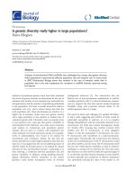
The true genetic diversity over the simulated genome,
calculated as the expected heterozygosity for the marker
locus within each marker interval (H

exp
_TRUE), ranged
from 0.04 to 0.53 with an average of 0.36 (Figure 2a). A
large number of H
exp
_TRUE values was found between
0.48 and 0.50 (Figure 3a), which is in accordance with a
population in Hardy-Weinberg equilibrium for an allele
frequency range 0.4-0.5.
Genetic diversity estimates
Genetic diversity estimated by IBD probabilities
(GD_IBD) varied considerably over the genome, with val-
ues ranging from 0.00 to 0.75, with an average of 0.52
(Figures 2b and 3b). Expected heterozygosity calculated
for the two adjacent marker loci around each marker
interval as an average (H
exp
_AVG) resulted in systemati-
cally lower values with a smaller range compared to
GD_IBD (0.05 to 0.50, average of 0.36) (Figures 2c and
3c). When expected heterozygosity was calculated for
flanking markers as a two-marker haplotype
(H
exp
_HAP2), the level and range of values increased and
were more similar to GD_IBD (0.05 to 0.75, average of
0.55) (Figures 2d and 3d). This result was expected, since
genetic diversity estimation with H
exp
_HAP2 is more

similar to GD_IBD because H
exp
_HAP2 also uses a haplo-
type construction, but with only two markers instead of
ten. Both heterozygosity estimates fluctuated more over
the genome compared to GD_IBD, reflecting a lower cor-
relation between values of adjacent marker intervals for
the heterozygosity estimates (H
exp
_AVG: r = 0.23;
H
exp
_HAP2: r = 0.28; GD_IBD: r = 0.64).
Comparison with true genetic diversity
The correlation between H
exp
_TRUE and GD_IBD was
weak (r = 0.21), and comparable to the correlations
between H
exp
_TRUE and H
exp
_AVG (r = 0.19) and
H
exp
_HAP2 (r = 0.20) (Table 1 and Figure 4). These
results indicate that both GD_IBD and heterozygosity
estimates are similar in predicting the genetic diversity
for ungenotyped regions of the genome in the current
simulated population. The correlation between GD_IBD

and H
exp
_AVG was 0.46, and was slightly higher between
GD_IBD and H
exp
_HAP2 (r = 0.49) (Table 1).
Comparison with true genetic diversity averaged over
marker intervals
When GD_IBD, H
exp
_AVG and H
exp
_HAP2 were aver-
aged over groups of marker intervals, the correlations
between H
exp
_TRUE and these estimates increased. They
were moderate when estimates were averaged over 40
marker intervals (r = 0.61-0.64, Table 1). Correlations of
all three estimates with H
exp
_TRUE were comparable to
each other. The correlation between GD_IBD and
heterozygosity estimates H
exp
_AVG and H
exp
_HAP2
increased with an increasing number of marker intervals,
and in the case of 40 marker intervals equalled 0.75 and

0.82, respectively. This indicates that GD_IBD, H
exp
_AVG
and H
exp
_HAP2 are similar in predicting the genetic
diversity for specific regions of the genome in a popula-
tion with a high marker density.
Influence of marker density
When genetic diversity over the genome was estimated in
a population with a lower marker density, the correlations
between the true genetic diversity and GD_IBD,
H
exp
_AVG and H
exp
_HAP2 changed, and turned out to be
slightly higher for GD_IBD (Table 2). This result suggests
that GD_IBD is a better predictor for genetic diversity
when using marker maps with a lower marker density.
Discussion
The aim of this paper was to compare two different esti-
mates of genetic diversity of a region lying in between
markers over the genome i.e. IBD-based genetic diversity
and heterozygosity. Genetic diversities estimated by IBD
probabilities and by heterozygosity of flanking markers
were positively correlated. The correlation of GD_IBD
and heterozygosity with the true genetic diversity was
quite similar for a simulated population with a high
marker density, for both specific and large regions over

the genome. For a population with a lower marker den-
sity, GD_IBD turned out to be a better predictor of
genetic diversity.
The assumption that is made for genetic diversity in the
ungenotyped marker interval is different for GD_IBD and
Engelsma et al. Genetics Selection Evolution 2010, 42:12
/>Page 6 of 10
Figure 2 a, b, c, d - Distribution of the estimated genetic diversity across the simulated genome. (a) True genetic diversity calculated by expect-
ed heterozygosity for the ungenotyped marker loci within the marker interval (H
exp
_TRUE); (b) Estimated genetic diversity with IBD probabilities be-
tween marker haplotypes (GD_IBD); (c) Estimated genetic diversity with expected heterozygosity as an average for the two flanking markers
(H
exp
_AVG); (d) Estimated genetic diversity with expected heterozygosity for the two flanking markers as a two marker haplotype (H
exp
_HAP2).






d c
b a
heterozygosity. With GD_IBD the assumption is that in
the base population relatedness was 0, i.e. all markers
were not-IBD and "heterozygosity" was 100%. With
heterozygosity, no such base population is assumed and
the assumption is that heterozygosity in the current gen-

eration for genotyped markers is predictive for ungeno-
typed markers. This explains why the average GD_IBD
estimated in this study was higher than the heterozygos-
ity estimates and the true heterozygosity. Heterozygosity
based on SNP markers with only two alleles will have,
under HWE, a maximum heterozygosity of 50% when the
minor allele frequency is 50%, as was simulated in this
study. For markers that have an unlimited number of
alleles, the true heterozygosity would probably be on
average closer to GD_IBD, while for markers with a low
diversity the true heterozygosity would be below both
GD_IBD and heterozygosity estimates.
When the genotyped marker is actually part of the gene
of interest, e.g., when the marker is a known QTL, then
heterozygosity at the marker fully determines the additive
genetic variance due to the QTL. In that case, additive
genetic variance due to the QTL simply equals H
exp
α
2
, α
denoting the allele substitution effect of the gene [5].
Hence, when markers coincide with genes of interest, i.e.
there are no QTL other than the genotyped markers,
there is no need to consider IBD probabilities. However,
in most cases, the genes of interest and their QTL will be
unknown, and it is unlikely that they coincide precisely
with genotyped markers. Consequently, prediction of
diversity in the ungenotyped regions between markers is
more relevant than the expected diversity at the markers,

because most genes of interest will be in the regions
between two markers. Such a prediction requires LD
between the genotyped markers and the regions in-
between markers, similar to the requirements in QTL
mapping [18]. Our results show that the IBD-based
method and heterozygosity are similar in using LD infor-
mation in the current simulated data with 1665 SNP
markers. However, when a population with a lower
marker density was used, GD_IBD became a slightly bet-
Engelsma et al. Genetics Selection Evolution 2010, 42:12
/>Page 7 of 10
Figure 3 a, b, c, d - Frequency of the estimated genetic diversity across the simulated genome. (a) True genetic diversity calculated by expected
heterozygosity for the ungenotyped marker loci within the marker interval (H
exp
_TRUE); (b) Estimated genetic diversity with IBD probabilities between
marker haplotypes (GD_IBD); (c) Estimated genetic diversity with expected heterozygosity as an average for the two flanking markers (H
exp
_AVG); (d)
Estimated genetic diversity with expected heterozygosity for the two flanking markers as a two marker haplotype (H
exp
_HAP2).





a b
c d
ter predictor of the genetic diversity in the marker inter-
val. In this second population the LD between markers is

low due to a larger marker distance, and in that case the
IBD-based method was expected to be a better predictor,
based on QTL mapping and genomic selection studies.
Explaining genetic diversity at a ungenotyped locus is
similar to the approaches of QTL mapping and genomic
selection, where the objective is to predict genetic vari-
ance at one or more unobserved QTL. In those
approaches, it has been shown that using an IBD-based
method to predict genetic variance at the unobserved
QTL is beneficial when the LD between the marker(s)
and the QTL is low, while this benefit disappears when
the LD increases [10,19].
In our study we ignored the non-segregating SNP
markers, as these markers are fixed in the simulated pop-
ulation and show no variation. This can be compared
with common practice where base pairs for which no
SNP markers are detected are considered uninformative.
However, we do not know whether this variation was
never there or existed in earlier generations and disap-
peared. In the latter case, these base pairs indicate a
genetic diversity of 0, and should not be ignored. In addi-
tion, when non-segregating markers are used in another
population, they might show variation and become infor-
mative. However, the correlations between the different
estimates for genetic diversity as estimated in this paper
are unlikely to be influenced by the exclusion of non-seg-
regating markers.
In this study, the estimation of genetic diversity was
done for a neutral genome without selection. The correla-
tion between genetic diversity estimates and true genetic

diversity was weak, but might increase if adaptive trait
variation is taken into account. The availability of dense
marker maps has opened up new possibilities to identify
reduced or increased levels of variability on specific
regions of the genome, associated to functional genes [8].
In case of selection, larger regions with less variation can
be found on the genome [20] and a better prediction of
the genetic diversity is possible.
Engelsma et al. Genetics Selection Evolution 2010, 42:12
/>Page 8 of 10
Figure 4 a, b, c - Relationship between the true genetic diversity (H
exp
_TRUE) and estimated genetic diversities. (a) by IBD probabilities be-
tween marker haplotypes (GD_IBD); (b) by expected heterozygosity as an average for the two flanking markers (H
exp
_AVG); (c) by expected heterozy-
gosity for the two flanking markers as a two marker haplotype (H
exp
_HAP2).





a b
c
How well the two methods predict genetic diversity
depends on the variation in diversity between adjacent
markers. In contrast to GD_IBD, the heterozygosity esti-
mates assume that diversity is similar for adjacent mark-

ers and for instance ignore recombination. When regions
of the genome form 'haplotype blocks', adjacent markers
have (near) identical diversity. In this case, heterozygosity
will better predict the genetic diversity. This was seen
when we simulated a population with an effective popula-
tion size of 100 instead of 1000, and 'haplotype blocks'
occurred due to the loss of variation. In this population
the correlation between the heterozygosity estimate
H
exp
_AVG and the true genetic diversity was higher com-
pared to the correlation between GD_IBD and the true
Table 1: Correlations of true genetic diversity (H
exp
_TRUE) with IBD-based diversity (GD_IBD) and heterozygosity
(H
exp
_AVG and H
exp
_HAP2).
MI
a
True vs. GD_IBD
b
True vs.
H
exp
_AVG
b
True vs.

H
exp
_HAP2
b
GD_IBD vs.
H
exp
_AVG
b
GD_IBD vs.
H
exp
_HAP2
b
1 0.20 0.19 0.20 0.46 0.49
4 0.33 0.27 0.28 0.54 0.58
10 0.46 0.37 0.38 0.64 0.70
20 0.56 0.47 0.50 0.73 0.80
40 0.62 0.61 0.64 0.75 0.82
a
The number of marker intervals taken into account to estimate the genetic diversity.
b
Correlations were calculated for values per marker interval, and for average values for a group of marker intervals (4, 10, 20 and 40 marker
intervals); for the latter, correlations were calculated for the true genetic diversity of even ungenotyped markers with the estimated genetic
diversity based on uneven (flanking) markers, and the other way around; the average of both correlations (even and uneven) is presented.
Engelsma et al. Genetics Selection Evolution 2010, 42:12
/>Page 9 of 10
genetic diversity (0.97 and 0.90, respectively). However,
when a population contains more variation, diversity in
between markers can be missed by heterozygosity, as

heterozygosity is only based on the variation of the mark-
ers itself. In that situation, GD_IBD also takes into
account the variation and possible recombination in
between markers, and is then expected to be a better esti-
mator of the genetic diversity over the genome. Conse-
quently, as shown in this study the method of choice will
also depend on the marker density [10,19], with high
marker densities (i.e. > 50 markers per cM) heterozygos-
ity is likely to perform better, with lower marker densities
(i.e. <10 markers per cM) GD_IBD is likely to perform
better.
Conclusions
In conclusion, the IBD-based method and heterozygosity
used to estimate genetic diversity of ungenotyped regions
of the genome (i.e. between markers) give similar results
for a simulated population with a high marker density.
However, for a population with a lower marker density,
the IBD-based method gives a better prediction, since
variation and recombination between markers are missed
with heterozygosity. IBD-based methods can provide
more insight in the genetic diversity of specific regions of
the genome, and subsequently contribute to select more
accurately the animals to be conserved, for example, to
construct a gene bank.
Competing interests
The authors declare that they have no competing interests.
Authors' contributions
KAE developed part of the programs used for analysis, carried out the simula-
tions and analyses, and wrote most of the paper. MPLC developed most of the
programs used for the simulations and analysis, and supervised and advised

KAE. PB contributed to part of the discussion and supervised and advised KAE.
JJW conceived the study, participated in its design and coordination, men-
tored and advised KAE daily, and contributed parts of the paper. All authors
took part in useful discussions, and provided useful advice on the analyses and
the first draft of the paper. All authors read and approved the final manuscript.
Acknowledgements
This study was financially supported by the Ministry of Agriculture, Nature and
Food (Programme "Kennisbasis Research", code: KB-04-002-021). The authors
would like to acknowledge Sipke Joost Hiemstra and Johan Van Arendonk for
their advice on the research and first draft of the paper, and Han Mulder for his
assistance in the analysis.
Author Details
1
Wageningen UR Livestock Research, Animal Breeding and Genomics Centre,
PO Box 65, 8200 AB Lelystad, The Netherlands,
2
Wageningen University,
Animal Breeding and Genomics Centre, PO Box 338, 6700 AH Wageningen, The
Netherlands and
3
Centre for Genetic Resources, The Netherlands (CGN), PO
Box 65, 8200 AB Lelystad, The Netherlands
References
1. Oldenbroek JK: Utilisation and conservation of farm animal genetic resources
Wageningen, The Netherlands: Wageningen Academic Publishers; 2007.
2. FAO: Global Plan of Action for Animal Genetic Resources and the Interlaken
Declaration 2007.
3. Woolliams JA, Toro M: What is genetic diversity? In Utilisation and
conservation of farm animal genetic resources Edited by: Oldenbroek JK.
Wageningen, The Netherlands: Wageningen Academic Publishers;

2007:55-74.
4. Toro MA, Caballero A: Characterization and conservation of genetic
diversity in subdivided populations. Philos Trans R Soc B-Biol Sci 2005,
360:1367-1378.
5. Falconer DS, Mackay TFC: Introduction to Quantitative Genetics Essex, UK:
Longman Group; 1996.
6. Meuwissen THE, Goddard ME: Prediction of identity by descent
probabilities from marker-haplotypes. Genet Sel Evol 2001, 33:605-634.
7. Reed DH, Frankham R: How closely correlated are molecular and
quantitative measures of genetic variation? A meta-analysis. Evolution
2001, 55:1095-1103.
8. Toro MA, Fernandez J, Caballero A: Molecular characterization of breeds
and its use in conservation. Livest Sci 2009, 120:174-195.
9. Fernando RL, Grossman M: Marker assisted selection using best linear
unbiased prediction. Genet Sel Evol 1989, 21:467-477.
10. Calus MPL, Meuwissen THE, de Roos APW, Veerkamp RF: Accuracy of
genomic selection using different methods to define haplotypes.
Genetics 2008, 178:553-561.
11. Meuwissen THE, Hayes BJ, Goddard ME: Prediction of total genetic value
using genome-wide dense marker maps. Genetics 2001, 157:1819-1829.
Received: 12 November 2009 Accepted: 10 May 2010
Published: 10 May 2010
This article is available from: 2010 Engelsma et al; licensee BioMed Central Ltd. This is an Open Access article distributed under the terms of the Creative Commons Attribution License ( which permits unrestricted use, distribution, and reproduction in any medium, provided the original work is properly cited.Genetics Selection Evolution 2010, 42:12
Table 2: Correlations of true genetic diversity (H
exp
_TRUE) with IBD-based diversity (GD_IBD) and heterozygosity
(H
exp
_AVG and H
exp

_HAP2), for a low marker density population (166 SNPs).
MI
a
True vs. GD_IBD
b
True vs.
H
exp
_AVG
b
True vs.
H
exp
_HAP2
b
GD_IBD vs.
H
exp
_AVG
b
GD_IBD vs.
H
exp
_HAP2
b
1 0.15 0.06 0.04 0.43 0.43
4 0.34 0.18 0.20 0.53 0.53
10 0.51 0.41 0.46 0.79 0.77
20 -
c

-
c
-
c
-
c
-
c
40 -
c
-
c
-
c
-
c
-
c
a
The number of marker intervals taken into account to estimate the genetic diversity.
b
Correlations were calculated for values per marker interval, and for average values for a group of marker intervals (4 and 10 marker intervals);
for the latter, correlations were calculated for the true genetic diversity of even ungenotyped markers with estimated genetic diversity based
on uneven (flanking) markers, and the other way around; the average of both correlations (even and uneven) is presented.
c
There were not enough estimates left over to calculate the correlation.
Engelsma et al. Genetics Selection Evolution 2010, 42:12
/>Page 10 of 10
12. Habier D, Fernando RL, Dekkers JCM: The impact of genetic relationship
information on genome-assisted breeding values. Genetics 2007,

177:2389-2397.
13. Windig JJ, Meuwissen THE: Rapid haplotype reconstruction in pedigrees
with dense marker maps. J Anim Breed Genet 2004, 121:26-39.
14. Meuwissen THE: Maximizing the response of selection with a
predefined rate of inbreeding. J Anim Sci 1997, 75:934-940.
15. Hill WG, Robertson A: Linkage disequilibrium in finite populations.
Theor Appl Genet 1968, 38:226-231.
16. De Roos APW, Hayes BJ, Spelman RJ, Goddard ME: Linkage
disequilibrium and persistence of phase in Holstein-Friesian, Jersey
and Angus cattle. Genetics 2008, 179:1503-1512.
17. Khatkar MS, Nicholas FW, Collins AR, Zenger KR, Al Cavanagh J, Barris W,
Schnabel RD, Taylor JF, Raadsma HW: Extent of genome-wide linkage
disequilibrium in Australian Holstein-Friesian cattle based on a high-
density SNP panel. 2008, 9:.
18. Dekkers JCM, Hospital F: The use of molecular genetics in the
improvement of agricultural populations. Nat Rev Genet 2002, 3:22-32.
19. Grapes L, Dekkers JCM, Rothschild MF, Fernando RL: Comparing linkage
disequilibrium-based methods for fine mapping quantitative trait loci.
Genetics 2004, 166:1561-1570.
20. Toro M, Maki-Tanila A: Genomics reveals domestication history and
facilitates breed development. In Utilisation and conservation of farm
animal genetic resources Edited by: Oldenbroek JK. Wageningen, The
Netherlands: Wageningen Academic Publishers; 2007:75-102.
doi: 10.1186/1297-9686-42-12
Cite this article as: Engelsma et al., Estimating genetic diversity across the
neutral genome with the use of dense marker maps Genetics Selection Evolu-
tion 2010, 42:12