Báo cáo sinh học: "Use of linear mixed models for genetic evaluation of gestation length and birth weight allowing for heavy-tailed residual effects" pptx
Bạn đang xem bản rút gọn của tài liệu. Xem và tải ngay bản đầy đủ của tài liệu tại đây (780.17 KB, 13 trang )
RESEARC H Open Access
Use of linear mixed models for genetic evaluation
of gestation length and birth weight allowing for
heavy-tailed residual effects
Kadir Kizilkaya
1,2*
, Dorian J Garrick
1,3
, Rohan L Fernando
1
, Burcu Mestav
2
, Mehmet A Yildiz
4
Abstract
Background: The distribution of residual effects in line ar mixed models in animal breeding applications is typically
assumed normal, which makes inferences vulnerable to outlier observations. In order to mute the impact of
outliers, one option is to fit models with residuals having a heavy-tailed distribution. Here, a Student’s-t model was
considered for the distribution of the residuals with the degrees of freedom treated as unknown. Bayesian
inference was used to investigate a bivariate Student’s-t (BSt) model using Markov chain Monte Carlo methods in a
simulation study and analysing field data for gestation length and birth weight permitted to study the practical
implications of fitting heavy-tailed distributions for residuals in linear mixe d models.
Methods: In the simulation study, bivariate residuals were generated using Student’s-t distribution with 4 or 12
degrees of freedom, or a normal distribution. Sire models with bivariate Student’s-t or normal residuals were fitted
to each simulated dataset using a hierarchical Bayesian approach. For the field data, consisting of gestation length
and birth weight records on 7,883 Italian Piemontese cattle, a sire-maternal grandsire model including fixed effects
of sex-age of dam and uncorrelated random herd-year-season effects were fitted using a hierarchical Bayesian
approach. Residuals were defined to follow bivariate normal or Student’s-t distributions with unknown degrees of
freedom.
Results: Posterior mean estimates of degrees of freedom parameters seemed to be accurate and unbiased in the
simulation study. Estimates of sire and herd variance s were similar, if not identical, across fitted models. In the field
data, there was strong support based on predictive log-likelihood values for the Student’s-t error model. Most of
the posterior density for degrees of freedom was below 4. Posterior means of direct and maternal heritabilities for
birth weight were smaller in the Student’s-t model than those in the normal model. Re-rankings of sires were
observed between heavy-tailed and normal models.
Conclusions: Reliable estimates of degrees of freedom were obtained in all simulated heavy-tailed and normal
datasets. The predictive log-likelihood was able to distinguish the correct model among the models fitted to
heavy-tailed datasets. There was no disadvantage of fitting a heavy-tailed model when the true model was normal.
Predictive log-likelihood values indicated that heavy-tailed models with low degrees of freedom values fitted
gestation length and birth weight data better than a model with normally distributed residuals.
Heavy-tailed and normal models resulted in different estimates of direct and maternal heritabilities, and different
sire rankings. Heavy-tailed models may be more appropriate for reliable estimation of genetic parame ters from field
data.
* Correspondence:
1
Department of Animal Science, Iowa State University, Ames, IA 50011 USA
Kizilkaya et al. Genetics Selection Evolution 2010, 42:26
http://( />Genetics
Selection
Evolution
© 2010 Kizilkaya et al; licensee BioMed Central Ltd. This is an O pen Access articl e distributed und er the terms of the Creative Commons
Attribution License ( which permits unrestricted use, di stribution, and reproduction in
any medium, provided the original work is pro perly cited.
Background
Animal breeding applicat ions commonly involve the fit-
ting of linear mixed models in order to estimate genetic
and phenotypic variation or to predict the genetic merit
of selection candidates. Measurement errors and other
sources of random non-genetic variation comprise the
residual term, the effects of which are often assumed to
be normally distributed with zero mean and common
variance. These assumptions may make inferences vul-
nerable to the presence of outliers [1,2]. Heavy-tailed
densities (such as Student’ s-t distribution) are viable
alternatives to the normal distribution, and provide
robustness against unusual or outlying observations
when used to model the densities of residual effects. In
the event that the degrees of freedom are estimated to
be large, i.e. in excess of 30, these methods converge to
normally distributed residuals [3].
Mixed effects linear models w ith Student’s-t distribu-
ted error effects have been applied to mute the impact
of residual outliers, for example in a situation where
preferential treatment of some individuals was suspected
[4]. Von Rohr and H oeschele [5] have demonstrated the
application of a Student’s-t sampling model under four
different error distributions in statistical mapping of
quantitative trait loci (QTL). They have determined that
additive and dominance QTL and residual variance esti-
mates are much closer to the simula ted true values
when the data itself is heavy-tailed and the ana lysis is
performed with the skewed Student’s-t model r ather
than with a normal model. Rosa et al. [6] have analyzed
birth weight in a reproductive toxicology study and
compa red normal as well as robust mixed linear models
based on Student’s-t distrib ution, Slash or contaminated
normal error distributions. Marginal posterior densities
of degrees of freedom for the Student’s-t and Slash
error distributions are concentrated about single digit
values, suggesting the inadequacy of the normal distri-
bution for modelling residual effects. The heavy-tailed
dis trib utions result in significantly better fit than a nor-
mal distribution. Kizilkaya et al. [3] have applied thresh-
old models with normal or Student’s- t link fu nctions for
the genetic analysis of calving ease scores and they have
shown that predictive log-likelihoods strongly favour a
Student’s-t model with low degrees of freedom in com-
parison with a normal distribution. Cardoso et al. [ 7]
have used heavy-tailed distributions to study residual
heteroskedasticity in beef cattle and have found that a
Student’s-t model s ignificantly improves predictive log-
likelihood value. Chang et al. [8] have compared multi-
variate heavy-tailed and probit threshold models in the
analysis of clinical mastitis in first lactation cows, and
have sho wn that a model comparis on strongly support s
the multivariate Slash and Student’s-t models with low
degrees of freedom over the probit model. The objec-
tivesofthisresearchwereto 1) examine by simulation
if Bayesian inference under a bivariate Student’s-t distri-
bution of residuals can accommodate models with either
light-tailed or heavy-tailed residuals, and 2) investigate
the practical implications of fitting a Student’s-t distri-
bution with unknown degrees of freedom for the resi-
duals in bivariate field data. In both cases, results we re
compared to those from the conventional approach of
assuming bivariate normal (BN) residuals.
Methods
We first present the theory and methods for multiple
traits that are applicable to both the simulation and the
analysis of field data on gestation length and birth
weight using a model that accommodates heavy-tailed
residuals.
Statistical model
A linear mixed model for animal i is
yXb a h
ii i i i
=++ +ZW
(1)
where y
i
=(y
i,1
y
i, m
)’ is a vector of phenotypic
values of animal i for m traits, b is a vector of fixed
effects, a is a vector of random genetic effects, h is a
vector of uncorrelated random effects such as herd
effects, X
i
, Z
i
and W
i
, are design matrices for animal i,
corresponding to the vectors of the fixed effects (b), ran-
dom genetic effects (a), and uncorrelated random effects
(h).
Conventional analyses might assume the vector
i
in
equation (1) is multivariate normally distributed (N(0,
R
0
)), where
R
0
2
2
11
1
=
⎛
⎝
⎜
⎜
⎜
⎜
⎞
⎠
⎟
⎟
⎟
⎟
eee
ee e
m
mm
.
In contrast, we assume
i
in (1) is multivariate heavy-
or light-tailed by expressi ng the residual in the usual
manner but divided by a scalar random variable that
varies for each animal i but is consistent across the
traits. That is,
11
1
2
1
2
m
i
m
i
i
i
i
e
e
⎛
⎝
⎜
⎜
⎜
⎞
⎠
⎟
⎟
⎟
=
⎛
⎝
⎜
⎜
⎜
⎞
⎠
⎟
⎟
⎟
=
−−
λλe ,
(2)
where l
i
in equation (2) is a positive random variable
[9]. Values of l
i
approaching 0 produce heavy-tailed
residuals for both traits, whereas values exceeding 1
Kizilkaya et al. Genetics Selection Evolution 2010, 42:26
http://( />Page 2 of 13
would produce light-tails. The marginal density of
i
is a
multivariate Stud ent’s-t density with scale parameter R
0
and df ν , such that the marginal residual variance
becomes
Var
iE
(| ,) RRR
00
2
==
−
⎛
⎝
⎜
⎞
⎠
⎟
[4,7,9].
Prior and full conditional posterior distributions
A flat prior was assumed for the fixed effects (b).
Genetic effects (a) were assumed to be distributed as
multivariate normal, with null mean vector and (co)var-
iance matrix A ⊗ G
0
where A is the numerator relation-
ship matrix and ⊗ denotes the Kronecker product [10].
Uncorrelated random effects and residuals were
assumed to follow multivariate normal distributions
with null means and (co)variance matrices I ⊗ H
0
and I
⊗ R
0
where I is the identity matrix. F lat prior dis tribu-
tions were assigned to G
0
, H
0
and R
0
.
The multivariate normal d istribution requires no dis-
tributional specification of l
i
in equation (2), because l
i
= 1 for all i = 1, 2, ,n. The distribution of l
i
in equation
(2) for multivariate Student’s-t is a Gamma(ν/2, ν/2) dis-
tribution with density function
p
v
i
i
v
i
λλλ|
(/)
/
(/)
exp ( )
(/)
()
=−
−
2
2
22
21
Γ
Where l
i
>0,Γ(.) is the standard Gamma function,
i = 1, 2, ,n and ν >0.Apriorof
p()
()
=
+
1
1
2
for ν >
0 was assigned to ν [3].
Inferences o n parameters of interest can be ma de
from the posterior distributions constructed using
MCMC methods such as Gibbs sampling or Metropolis-
Hastings [11-13]. The fully conditional posterior distri-
butions of each of the unknown parameters are used to
generate proposal samples from the target distribution
(the joint posterior). The fully conditional posterior dis-
tributions of fixed (b), genetic (a) and uncorrelated ran-
dom (h) effects are multivariate normal with mean
[,, ]bah
∧∧∧
and covariance matrix C,where
[,, ]bah
∧∧∧
are
solutions to Henderson’ s mixed model equations con-
structed with he terogeneous residual variances,
R
0
λ
i
-1
and C is the inverse of this mixed-model coefficient
matrix [4]. The (co)variance matrices G
0
, H
0
and R
0
have inverse Wishart conditi onal posterior distribution s,
which can also be constructed from
[,, , ]bah
∧∧∧ ∧
where
∧
is solution for l
i
[9].
The fully conditional posterior distributions of l
i
for
the multivariate Student’s-t model is
Gamma
m
+
′
+
⎛
⎝
⎜
⎞
⎠
⎟
−
2
1
2
0
1
,[ ]eR e
where e = y
i
- X
i
b - Z
i
a - W
i
h.
The fully conditional posterior distribution of df ν for
the multivariate Student’ s-t model does not have a stan-
dard form, and so a sampling strategy for nonstandard
distributions is required. A random-walk Metropolis-
Hastings (MH) algorithm was used to draw samples for
ν [11]. In the MH algorithm, a normal density with
expectation equal to the parameter value from the pre-
viousMCMCcyclewasusedastheproposaldensity.
The MH acceptance ratio was tuned to intermediate
rates (40-50%) during the MCMC burn-in period to
optimize MCMC mixing [3]. Sampled values of ν <2
were truncated to 2 so that covariance matrix,
RR
E
=
()
−
0
2
, for the residuals of (1) is defined.
Simulation study
A simulation study was carried out to validate Bayesian
inference on the b ivariate Student’s-t models, and assess
the ability of model choice criterion (predictive log-likeli-
hood) to correctly choose the model with better fit. For
this purpose, the simulation study was undertaken using
three sire models to simulate the bivariate data, these
models varying in the nature of the simulated residual
effects. We refer to the model used to simulate the data
as the true model. These three models were the bivariate
normal which effectively has infinite ν (BN-∞)andthe
bivariate Student’s-t model with ν =4or12(BSt-4, BSt-
12). Ten replicated data sets were generated for each of
the three true models. Phenotypes of 50 progeny from
each of 50 unrelated sires for two traits, y
i
=(y
i,1
y
i,2
)’
were simulated using equation (1). The vector of fixed
effects b only included a gender effect with b
1
= (11 90)’
for trait 1 and b
2
= (38 32)’ for trai t 2. The ran dom
genetic effects (a) and uncorrelated random effects (h)
included 50 sires and 100 herds, respectively, assuming:
a
h
GI 0
0HI
0
0
⎛
⎝
⎜
⎞
⎠
⎟
⎡
⎣
⎢
⎤
⎦
⎥
⊗
⊗
⎡
⎣
⎢
⎤
⎦
⎥
⎛
⎝
⎜
⎜
⎞
⎠
⎟
⎟
N ,
0
0
where G
0
is the sire (co)variance matrix,
G
0
2
2
1
21 2
12
20 15
15 40
=
⎛
⎝
⎜
⎜
⎞
⎠
⎟
⎟
=
⎛
⎝
⎜
⎞
⎠
⎟
sss
ss s
,
and H
0
is the herd (co)variance matrix
H
0
2
2
1
2
0
0
15 0
060
=
⎛
⎝
⎜
⎜
⎞
⎠
⎟
⎟
=
⎛
⎝
⎜
⎞
⎠
⎟
h
h
.
.
.
Residuals were assumed e
i
~ N (0, R
0
), where
R
0
2
2
112
21 2
15 0 4 0
40 200
=
⎛
⎝
⎜
⎜
⎞
⎠
⎟
⎟
=
⎛
⎝
⎜
⎞
⎠
⎟
eee
ee e
.
Kizilkaya et al. Genetics Selection Evolution 2010, 42:26
http://( />Page 3 of 13
Heritabilities of simulated traits were
h
1
2
043= .
and
h
2
2
053= .
, respectively. For each animal i, l
i
was 1 for
BN-∞ or generated from Gamma(ν/2, ν/2) for BSt - ν with
ν = 4, 12. Offspring were assigned to herd and gender
groups by random sampling from a uniform distribution.
Gestation length and birth weight data
Gestation length (GL) up until first calving and the resul-
tant calf birth weight (BW) data were recorded on the
national population of Italian Piemontese cattle from Jan-
uary 1989 to July 1998 by Associazione Nazionale Alleva-
tori Bovini di Razza Piemontese (ANABORAPI), Strada
Trinità 32a, 12061 Carrù, Italy. Only herds re presented
by at least 100 records over that period were considered
in the study [14], providing a total of 7,883 animals from
677 sires and 747 MGS. Table 1 summarizes the statistics
for GL and BW. BSt and BN models given in equation (1)
were used to analyze GL and BW data. The fixed effects
(b) of dam age in months, sex of the calf, and their inter-
action were considered by combining eight different first-
calf age group classes (20 to 23, 23 to 25, 25 to 27, 27 to
29,29to31,31to33,33to35,and35to38months)
with sex of calf for a total of 16 nominal age-sex sub-
classes. A total of 1,186 herd-year-season (HYS) sub-
classes were created from combinations of herd, year,
and two different seasons (from November to April and
from May to October) as in Carnier et al. [15] and Kizilk-
aya et al., [3] and treated as uncorrelated random effects
( h) [14]. The range for number of observations in HYS
subclasses was between 1 and 33, and average number of
records for HYS effect was 7. The random genetic effects
(a) included 1,929 sires (s)andMGS(m)fromthepedi-
gree file. While the number of observations ranged from
1 to 406, average observations for each sire in data file
was 12. We also assumed:
a
h
GA 0
0HI
0
0
⎛
⎝
⎜
⎞
⎠
⎟
⎡
⎣
⎢
⎤
⎦
⎥
⊗
⊗
⎡
⎣
⎢
⎤
⎦
⎥
⎛
⎝
⎜
⎜
⎞
⎠
⎟
⎟
N
,
0
0
where G
0
is the sire-MGS (co)variance matrix,
G
0
2
2
2
=
s
ss
mD ms m
mm mm
GL
BW
S
GL
BW
GL GL GL BW GL
BW
S
GL BW
S
BW
BW GGL BW
m
2
⎛
⎝
⎜
⎜
⎜
⎜
⎜
⎜
⎜
⎞
⎠
⎟
⎟
⎟
⎟
⎟
⎟
⎟
and H
0
is the HYS (co)variance matrix,
H
0
2
2
0
0
=
⎛
⎝
⎜
⎜
⎞
⎠
⎟
⎟
h
h
GL
BW
.
Marginal residual variances, heritabilities and genetic
correlations
Residual scale par ameters (R
0
) in heavy-tailed models
cannot be directly compared with the residual (co)var-
iance (R
0
) in the normal model, nor used in estimation of
heritabilities, residual orphenotypiccorrelations.
The scale parameters must be appropriately transformed
into marginal residual ( co)variance parameters
R
E
EEE
EE E
GL GL BW
BW GL BW
=
⎛
⎝
⎜
⎜
⎞
⎠
⎟
⎟
2
2
for BN and BSt models, using
R
E
= R
0
and
RR
E
=
()
−
0
2
where ν > 2, respectively,
given by Stranden and Gianola [4] and Cardoso et al. [7].
Heritabilities and genetic correlations are of interest
from the perspective of direct and maternal effects in an
animal model, but the fitted models for GL and BW
included genetic effects for sire and MGS, and some
fractions of the genetic effects were included in the resi-
dual terms. Transfo rmations were applied to convert the
sire-MGS parameters and estimates to their animal
model equivalent. The additive genetic (co)variance
matrix including direct (D)andmaternal(M)genetic
variances from sire-MGS model was obtained as G
DM
=
PG
0
P′ [16] where G
DM
is an additive genetic (co)var-
iance matrix,
G
DM
D
DD D
MD MD M
MD MD M
GL
BW GL BW
GL GL GL BW GL
BW GL BW BW BW
=
2
2
2
MMM
GL BW
2
⎛
⎝
⎜
⎜
⎜
⎜
⎜
⎜
⎞
⎠
⎟
⎟
⎟
⎟
⎟
⎟
and P is an appropriate transformation matrix,
P =
−
−
⎛
⎝
⎜
⎜
⎜
⎜
⎜
⎞
⎠
⎟
⎟
⎟
⎟
⎟
2 000
0 200
2 020
0 202
.
Direct and maternal (
h
G
ij,
2
) heritability, and genetic
correlation (
r
GG
ij kj,,
′
) estimates were obtained from esti-
mates of variance and covariance components according
to:
Table 1 Summary statistics for gestation length (GL) and
birth weight (BW) in Italian Piemontese cattle
Trait N Mean Minimum Maximum SD
GL (day) 7,883 290 260 320 8.1
BW (kg) 7,883 39.6 22 56 4.1
Kizilkaya et al. Genetics Selection Evolution 2010, 42:26
http://( />Page 4 of 13
h
G
ij
s
ij
s
ij
m
ij
m
ij
h
ij
E
ij
G
ij,
,
,
,,
,,,
2
2
2
2
222
=
++++
and
r
GG
GG
GG
ij kj
ij kj
ij ij
,,
,,
,,
′
′
′
=
22
Where G and G′ = D or M, i and k for the trait of GL
or BW and j for the model of BN or BSt.
Kendall r ank correlations between posterior means of
sire genetic effects obta ined from the BN and BSt mod-
els were used to compare the ordering of the genetic
evaluations of the sires for GL and BW [17]. Compari-
sons were also made between rank orders of the top
100 selection candidates fr om 1,929 animals in the pedi-
gree file for the BN model.
Model comparison
Model comparisons in the simulation study, and for the
analysis of field data, were carried out using predictive
log-likelihoods (PLL) from BN and BSt models. The
PLL over all observations (n)underModelM
k
(k =BN
or BSt) was obtained as:
PLL p M
G
pM
k
i
n
i
i
k
i
n
j
G
i
j
k
=
()
=
()
=
()
=
−
=
∑
∑∑
log | ,
log | ,
()
1
1
1
1
1
yy
y
⎛⎛
⎝
⎜
⎜
⎞
⎠
⎟
⎟
−1
(3)
where
((|,))
()
1
1
1
1
G
pM
j
G
i
j
k
−
=
−
∑
y
is the harmonic
mean of p
-1
(y
i
|θ
(j)
, M
k
)acrossG MCMC samples [18].
A PLL diffe rence exceeding 2.5 was used a s indication
of an important difference in model fit, following Raftery
[19].
In the simulation study, the impact of alternative
models was quantified by computing the correlations
(r
â, a
) between the simulated true (a) and predicted (â)
sire effects in each of the three fitted models. Further,
the prediction error variance (PEV) V(a - â)) of the sire
effects was calculated to provide an informative com-
parative assessment of model prediction performance.
Higher correlations and lower prediction error variances
will be associated with fitted models that are better at
predicting breeding values than models with low corre-
lations and high prediction error variance. Some fitted
models might be significantly better than others from a
likelihood framework, yet have little impact on selection
response if they do not markedly change correlations.
Minimizing the prediction error variances is important
when investment decisions depend upon the magnitude
of the sire predictions, not just the ranking of the sires.
MCMC implementation
Graphical inspection (time series traces) of the chains
along with Heidelberger and Welch Diagnostic [20] for
the Gibbs output using CODA (Convergence Diagnostics
andOutputAnalysispackageinR)[21]wereusedto
determine a commo n length of burn-in period. A burn-
in period of 50,000 for simulated and field data analysis
was defined as the number of cycles discarded at the
start of the MCMC chain to ensure sampling from the
correct marginal distributions. A further 50,000 post
burn-inMCMCcyclesinthesimulatedandfielddata
analysis were generated for each of the BSt and BN mod-
els. Every successive post burn-in sample was retained, so
that 50,000 samples were used to infer posterior distribu-
tions of unknown parameters. Posterior means of the
parameters were obta ined from their respective margina l
posterior densities. Interval estimates were determined as
posterior probability intervals (PPI) obtained from the 2.5
and 97.5 percentiles of each posterior density to provide
95% PPI. The effective number of independent samples
(ESS) for each parameter was determined using the initial
positive sequence estim ator of Geyer [22] as adapted by
Sorensen et al. [23].
Results and discussion
Simulation study
The predictive log-likelihood values in Table 2 were com-
puted for BSt and BN m odels fitted to the simulated
heavy-tailed and normal datasets. When the true model
had residuals with heavy-tails, the fitted models with
heavy-tails (BSt) were significantly better than the normal
model (BN). When the true model had normally distribu-
ted residuals, all the fitted models performed equally well.
The difference in PLL between the fitted models w ith
heavy-tails and the normal model was inversely related to
the degrees of freedom of the simulated residuals. Note
Table 2 Comparisons of average predictive log-
likelihood
1
(PLL) from ten replicates between bivariate
Student’s-t (BSt) and normal (BN) fitted models (in
column) for different true simulated models (in rows)
with varying residual degrees of freedom (DF)
Fitted Model
3
True Model
2
-DF BSt BN
BSt-4 -1,483 -1,988
BSt-12 -718 -754
BN-∞ -284 -284
1
Predictive log-likelihood values were reported after adding 14,000
2
Used to simulate data
3
Used in analysis of simulated data
Kizilkaya et al. Genetics Selection Evolution 2010, 42:26
http://( />Page 5 of 13
that normally distributed residuals can be thought of as
having infinite degrees of freedom, and in this case there
were no differences between the fitted models.
Inference on ν based on BSt model analysis of BSt-4,
BSt-12 and BN-∞ data sets is given in Table 3. Posterior
means of ν seems sharp and unbiased, and the 95% pos-
terior probability intervals for ν concentrated on low
values for BSt-4 and BSt-12 data sets. Conversely, infer-
ence on ν for BN-∞ data was larger than 100, consistent
with what was expected, and the 95% posterior probabil-
ity interval was wider by concentrating on values higher
than 30, indicating strong evidence of normally distribu-
ted data. Furthermore, relatively larger ESS of ν were
obtained from BSt-4 and BSt-12 data sets when com-
pared with that from BN-∞ data sets [3], in dicating more
samples would be needed to attain a minimum of 100 as
advocated by Bink et al. [24] and Uimari et al. [25].
Tables4,5and6summarizeinferencesonsire,herd
and marginal error variances based on the replicated
datasets from the three different populations, comparing
BSt and BN fitted models. Large ESS were attained for
sire, herd and marginal error variances, indicating stable
MCMC inference. The 95% post erior probability inter-
vals for sire and herd variance components from the
three fitted models widely overlapped and included the
true parameter values. Furthermore, the posterior means
from the three fitted models were almost identical.
When the true model was BSt-4 or BN-∞, inferences on
marginal error (co)varianc e components using the BSt
and BN fitted models were similar, found to be sharp
and seemingly unbiased, and true parameter values were
covered by 95% equal-tailed PPI of parameters (Table 6).
Average correlations between true and e stimated sire
effects and average PEV from two replicates using BSt
and BN fitted models are presented i n Table 7 and 8.
When the true model was BSt, both the corre lation and
PEV indicate that the heavy-tailed fitted models were
superior, especially when the true value of ν =4.When
the true model was BN, all fitted models performed
identically. In general, the accuracy and PEV results
from BSt and BN models suggest that heavy-tailed fitted
models can improve accuracy and PEV when the true
model is heavy-tailed, but a robust Bayesian analysis
using heavy-tailed models does not deteriorate accuracy
and PEV if the true model is normal.
Application to gestation length and birth weight
Inference on degrees of freedom, variance components and
heritabilities
The analyses produced PLL values for BSt and BN mod-
els of -47,006 and -48,006 respectively. The log-scale
differences between model PLL values for BSt versus
BN models were 1,000, which greatly exceeds 2.5 and
Table 3 Average posterior inference on degrees of
freedom from ten replicates using the bivariate
Student’s-t (BSt) fitted model
BSt Fitted Model
2
True Parameters True Model
1
PM ± SE
3
95% PPI
4
ESS
5
ν =4 BSt-4 4.1 ± 0.06 [3.6, 4.6] 1,594
ν =12 BSt-12 13.3 ± 1.18 [9.8, 19.1] 294
ν = ∞ BN-∞ 2377 ± 654 [2140, 3365] 14
1
Used to simulate data
2
Used in analysis of simulated data
3
Posterior mean ± Standard Error
4
95% equal-tailed posterior probability interval based on the 2.5
th
and 97.5
th
percentiles of the posterior density
5
Effective sample size
Table 4 Average posterior inference on sire (co)variances from ten replicates using the bivariate Student’s-t (BSt) and
normal (BN) fitted models with different residual degrees of freedom (DF)
Fitted Model
2
BSt BN
True Parameters True Model
1
PM ± SE
3
95% PPI
4
ESS
5
PM ± SE 95% PPI ESS
s
1
2
= 2.0 BSt-4 2.24 ± 0.16 [1.32, 3.62] 20,983 2.31 ± 0.18 [1.30, 3.83] 20,694
BSt-12 2.44 ± 0.14 [1.48, 3.88] 24,767 2.39 ± 0.14 [1.44, 3.81] 25,794
BN-∞ 2.49 ± 0.17 [1.52, 3.93] 26,715 2.49 ± 0.17 [1.53, 3.93] 28,154
ss
12
= 1.5 BSt-4 1.41 ± 0.17 [0.40, 2.76] 23,326 1.43 ± 0.18 [0.33, 2.89] 23,146
BSt-12 1.93 ± 0.19 [0.83, 3.47] 27,428 1.89 ± 0.19 [0.80, 3.42] 28,683
BN-∞ 1.77 ± 0.22 [0.72, 3.23] 28,441 1.77 ± 0.21 [0.71, 3.22] 30,064
s
2
2
= 4.0 BSt-4 4.23 ± 0.30 [2.59, 6.70] 24,192 4.33 ± 0.33 [2.57, 6.99] 23,978
BSt-12 4.77 ± 0.29 [2.97, 7.48] 27,674 4.80 ± 0.30 [2.98, 7.55] 29,102
BN-∞ 4.46 ± 0.39 [2.79, 6.96] 29,013 4.45 ± 0.39 [2.78, 6.98] 29,365
1
Used to simulate data
2
Used in analysis of simulated data
3
Posterior mean ± Standard Error
4
95% equal-tailed posterior probability interval based on the 2.5
th
and 97.5
th
percentiles of the posterior density
5
Effective sample size
Kizilkaya et al. Genetics Selection Evolution 2010, 42:26
http://( />Page 6 of 13
decisively indic ates the inadequacy of the normality
assumption for the distribution of error terms. These
results are in agreement with Chang et al. [8] and C ar-
doso et al. [17], who found that the Student’s-t distribu-
tion was a better fit to the clinical mastitis data and
postweaning gain data, respectively, compared to Slash
and normal distributions.
The estimated ESS for ν is 1,227 and those for va r-
iance components are given in Tables 9, 10 and 11. The
ESS for these parameters r anged from 323 to 15,789,
indicating sufficient MCMC mixing. These values were
found to be considerably higher than 100, which has
been suggested as the minimum ESS for reliable statisti-
cal inference [24,25].
The posterior distribution of ν from the BSt model,
and its posterior mean (M) and 95% PPI corresponding
to the 2.5 (L) and 97.5 (U) percentiles of the posterior
distribution are in Figure 1. The posterior mean of ν for
the BSt model was 3.70, with 95% PPI of (3.44, 3.97).
This density, characterized by small values of ν fo r BSt
model confirms that the assumption of normally distrib-
uted residuals is not adequate for the analysis of
Piemontese GL and BW data.
Posterior inferences on sire-MGS and HYS (co)var-
iances for GL and BW are summarized in Tables 9 and
10, using po sterior means and 95% PPIs from BSt and
BN models. Posterior distributions of (co)variances were
nearly symmetric in BSt and BN models. Posterior
means of sire-MGS (co)variances were similar across
models, and 95% P PI widely overlapped. Posterior
means of sire-MGS (co)variances from BN model, how-
ever, were lower than that from BSt m odel for GL, and
were larger than that from BSt model for BW. Cova r-
iances from BN model, including sire or MGS effect for
Table 5 Average posterior inference on herd variances from ten replicates using the bivariate Student’s-t (BSt) and
normal (BN) fitted models with different residual degrees of freedom (DF)
Fitted Model
2
BSt BN
True Parameters True Model
1
PM ± SE
3
95% PPI
4
ESS
5
PM ± SE 95% PPI ESS
h
1
2
= 1.5 BSt-4 1.71 ± 0.10 [1.07, 2.56] 12,027 1.74 ± 0.14 [1.01, 2.71] 10,437
BSt-12 1.82 ± 0.12 [1.19, 2.65] 16,133 1.82 ± 0.12 [1.18, 2.65] 16,802
BN-∞ 1.71 ± 0.08 [1.12, 2.48] 17,543 1.70 ± 0.08 [1.12, 2.47] 17,537
h
2
2
= 6.0 BSt-4 6.33 ± 0.30 [4.47, 8.79] 24,120 6.49 ± 0.28 [4.47, 9.17] 22,810
BSt-12 6.69 ± 0.28 [4.77, 9.22] 27,704 6.72 ± 0.24 [4.79, 9.28] 27,956
BN-∞ 6.33 ± 0.27 [4.55, 8.71] 29,800 6.33 ± 0.27 [4.55, 8.71] 29,881
1
Used to simulate data
2
Used in analysis of simulated data
3
Posterior mean ± Standard Error
4
95% equal-tailed posterior probability interval based on the 2.5
th
and 97.5
th
percentiles of the posterior density
5
Effective sample size
Table 6 Average posterior inference on marginal error (co)variances from ten replicates using the bivariate Student ’s-
t (BSt) and normal (BN) fitted models with different residual degrees of freedom (DF)
Fitted Model
2
BSt BN
True Parameters True Model
1
PM ± SE
3
95% PPI
4
ESS
5
PM ± SE 95% PPI ESS
E
1
2
= 30.0 BSt-4 30.45 ± 0.51 [27.44, 34.05] 3,336 30.29 ± 0.44 [28.61, 32.07] 42,430
E
1
2
= 18.0 BSt-12 17.87 ± 0.17 [16.75, 19.07] 9,516 17.82 ± 0.16 [16.83, 18.87] 43,135
E
1
2
= 15.0 BN-∞ 14.94 ± 0.11 [14.10, 15.82] 43,387 14.94 ± 0.11 [14.11, 15.82] 43,204
EE
12
= 8.0 BSt-4 8.20 ± 0.38 [6.45, 10.10] 11,384 8.37 ± 0.66 [6.95, 9.83] 44,553
EE
12
= 4.8 BSt-12 4.61 ± 0.13 [3.69, 5.56] 32,416 4.57 ± 0.12 [3.72, 5.44] 44,370
EE
12
= 4.0 BN-∞ 3.94 ± 0.10 [3.23, 4.67] 43,729 3.94 ± 0.10 [3.23, 4.66] 44,238
E
2
2
= 40.0 BSt-4 40.07 ± 0.65 [35.98, 44.94] 3,566 39.57 ± 0.74 [37.37, 41.90] 45,168
E
2
2
= 24.0 BSt-12 24.60 ± 0.31 [23.04, 26.27] 10,145 24.54 ± 0.28 [23.17, 25.98] 45,130
E
2
2
= 20.0 BN-∞ 20.13 ± 0.18 [19.00, 21.31] 42,782 20.12 ± 0.18 [19.00, 21.31] 45,079
1
Used to simulate data
2
Used in analysis of simulated data
3
Posterior mean ± Standard Error
4
95% equal-tailed posterior probability interval based on the 2.5
th
and 97.5
th
percentiles of the posterior density
5
Effective sample size
Kizilkaya et al. Genetics Selection Evolution 2010, 42:26
http://( />Page 7 of 13
BW with sire or MGS effect for GL were higher than
thos e from BSt and BS models. Posterior means of HYS
variances from BSt an d BN models were similar and
ranged from 4 to 4.25 for GL, and 2.43 to 2.56 for BW
from the two models. Posterior inference for the mar-
ginal residual (co)variances based on BSt and BN m od-
els are presented in Table 11. The marginal residual
variance for GL, and covariance between GL and BW
from BSt model seemed to agre e with those from the
BN model; however, the posterior mean of marginal
residual variance for BW from the BSt model was signif-
icantly higher than that of the BN model.
Posterior densities of direct and maternal heritabilities,
and genetic correlations from BSt and BN models for
GLandBWareshowninFigures2and3.Posterior
means of direct (0.47) and maternal (0.29) heritabilities
from BSt and BN models were similar for GL. However,
posterior means of direct (0.28) and maternal (0.23) her-
itabilities from BN models were higher than those (0.23
and 0.18) from the heavy-tailed model for BW (Figure
2). In contrast to our fi ndings, Cardoso et al . [7] and
Chang et al. [8] have found no real difference in poster-
ior means for heritabilities whether using Student’ s-t,
Slash or normal models. P osterior means of direct herit-
abilities from BSt and BN models for GL and BW traits
were lower; however, those of maternal heritabilities
were higher than the values reported by Ibi et al. [26]
and Crews [27]. Posterior means (-0.87, -0.86) of genetic
correlations between D and M effects of GL, and those
(-0.73, -0.71) of BW from BSt and BN models in Figure
3 were significantly negative and very similar with over-
lapping posterior densities. They were higher than those
repo rted in literature [26,27], and the negative posterior
mean of the genetic correlation implies an antagonistic
relationship between D and M effects. The posterior
Table 7 Average correlations between true and predicted
sire effects from ten replicates using the bivariate
Student’s-t (BSt) and normal (BN) fitted models with
different residual degrees of freedom (DF)
Fitted Model
2
Trait1 Trait2
True Model
1
-DF BSt BN BSt BN
BSt-4 0.90 0.87 0.92 0.90
BSt-12 0.93 0.93 0.95 0.95
BN-∞ 0.94 0.94 0.95 0.95
1
Used to simulate data
2
Used in analysis of simulated data
Table 8 Prediction error variance of sire effects using the
bivariate Student’s-t (BSt) and normal (BN) fitted models
with different residual degrees of freedom (DF)
Fitted Model
2
Trait1 Trait2
True Model
1
-DF BSt BN BSt BN
BSt-4 0.36 0.44 0.51 0.67
BSt-12 0.29 0.30 0.41 0.44
BN-∞ 0.23 0.23 0.33 0.33
1
Used to simulate data
2
Used in analysis of simulated data
Table 9 Posterior inference on sire-MGS (co)variances for
gestation length (GL) and birth weight (BW) using the
bivariate Student’s-t (BSt) and normal (BN) models
BSt BN
Parameters PM
1
95% PPI
2
ESS
3
PM 95% PPI ESS
s
GL
2
8.42 [6.65, 10.43] 894 8.13 [6.27, 10.31] 384
ss
GL BW
0.13 [-0.43, 0.72] 774 0.16 [-0.48, 0.81] 496
sm
GL GL
2.75 [1.77, 3.76] 567 2.73 [1.63, 3.81] 323
sm
GL BW
-0.54 [-1.04, -0.04] 524 -0.74 [-1.32, -0.21] 405
s
BW
2
1.02 [0.68, 1.43] 528 1.12 [0.75, 1.55] 550
sm
BW GL
0.26 [-0.13, 0.69] 429 0.40 [-0.09, 0.90] 230
sm
BW BW
0.36 [0.15, 0.58] 428 0.39 [0.18, 0.62] 484
m
GL
2
2.24 [1.47, 3.16] 389 2.04 [1.17, 3.05] 232
mm
GL BW
0.27 [-0.03, 0.57] 430 0.32 [-0.01, 0.69] 336
m
BW
2
0.53 [0.34, 0.74] 457 0.59 [0.38, 0.87] 371
1
Posterior mean
2
95% equal-tailed posterior probability interval based on the 2.5
th
and 97.5
th
percentiles of the posterior density
3
Effective sample size
Table 10 Posterior inference on herd-year-season (co)
variances for gestation length (GL) and birth weight (BW)
using the bivariate Student’s-t (BSt) and normal (BN)
models
BSt BN
Parameters PM
1
95% PPI
2
ESS
3
PM 95% PPI ESS
h
GL
2
4.00 [3.02, 5.10] 2,122 4.21 [3.00, 5.60] 1,661
h
BW
2
2.43 [2.04, 2.85] 3,282 2.56 [2.14, 3.00] 3,403
1
Posterior mean
2
95% equal-tailed posterior probability interval based on the 2.5
th
and 97.5
th
percentiles of the posterior density
3
Effective sample size
Table 11 Posterior inference on marginal residual (co)
variances for gestation length (GL) and birth weight (BW)
using the bivariate Student’s-t (BSt) and normal (BN)
models
BSt BN
Parameters PM
1
95% PPI
2
ESS
3
PM 95% PPI ESS
E
GL
2
51.86 [48.43, 55.84] 2,376 48.90 [47.22, 50.64] 9,039
EE
GL BW
3.77 [3.01, 4.56] 8,213 3.20 [2.63, 3.78] 11,671
E
BW
2
13.37 [12.47, 14.41] 2,367 11.14 [10.76, 11.53] 15,789
1
Posterior mean
2
95% equal-tailed posterior probability interval based on the 2.5
th
and 97.5
th
percentiles of the posterior density
3
Effective sample size
Kizilkaya et al. Genetics Selection Evolution 2010, 42:26
http://( />Page 8 of 13
densities of genetic correlations between D effects o n
one trait and M effects on another included zero, indi-
cating non-significant correlations.
The posterior means of l
i
in the BSt model can be used
to assess the e xtent to which any particul ar pair of
records presents an outlier for either trait in comparison
to a normal error assumption. Low values of l
i
(i.e. closer
to zero) indicate at least one deviant record among the
two traits, whereas values of l
i
close to 1 show that the
corresponding pair of records match the norma l model
[17]. The ranges of posterior means of l
i
obtained for dif-
ferent animals from the BSt models varied between 0.09
and 1.75. The values of l
i
are plotted against estimated
values of residuals for BW and GL in Figure 4. The distri-
butions of posterior means of l
i
less than 0.3 (left figure)
or less than 0.2 (right figure) are given in Figure 4. The
figure on the right plots posterior mean values of l
i
less
than 0.2, representing ou tliers 3 or more standard devia-
tions (SD) from the mean for GL or BW. When the pos-
terior mean values of l
i
are close to unity, the estimated
values of residuals approach normally distributed resi-
duals, indicating adequate model fit.
In general, random effects contributing to bivariate
traits may be correlated positively, negatively or uncor-
related. Accordingly, it is reasonable that effects may
Student's t Distribution
Degrees of Freedom
Density
0.0
0.5
1.0
1.5
2.0
2.5
3.0
3.2 3.4 3.6 3.8 4.0 4.2
LM U
Figure 1 Posterior densities of degrees of freedom obtained
from bivariate Student’s-t (BSt) model fitted to gestation
length (GL) and birthweight (BW). M represents posterior mean, L
represents the 2.5
th
percentiles of the posterior density, U represent
97.5
th
percentiles of the posterior density.
Gestation Length
h
2
D
Density
0
2
4
6
8
0.2 0.4 0.6 0.8
BN BSt
Birth Weight
h
2
D
Density
0
2
4
6
8
10
0.2 0.4 0.6 0.8
BN BSt
h
2
M
Density
0
2
4
6
0.2 0.4 0.6 0.8
h
2
M
Density
0
2
4
6
8
0.2 0.4 0.6 0.8
Figure 2 Posterior densities of direct (D) and maternal (M) heritabilities of gestation length (GL) and birth weight (BW) obtained from
bivariate Student’s-t (BSt) or normal (BN) models.h
2
D and h
2
M represent direct and maternal heritabilities.
Kizilkaya et al. Genetics Selection Evolution 2010, 42:26
http://( />Page 9 of 13
r(GL_D,GL_M)
Density
0
2
4
6
8
10
-1.0 -0.8 -0.6 -0.4 -0.2 0.0 0.2 0.4 0.6 0.8 1.0
r(BW_D,BW_M)
Density
0
1
2
3
4
5
-1.0 -0.8 -0.6 -0.4 -0.2 0.0 0.2 0.4 0.6 0.8 1.0
r(GL_D,BW_D)
Density
0
1
2
3
4
-1.0 -0.8 -0.6 -0.4 -0.2 0.0 0.2 0.4 0.6 0.8 1.0
r(GL_M,BW_M)
Density
0.0
0.5
1.0
1.5
2.0
2.5
-1.0 -0.8 -0.6 -0.4 -0.2 0.0 0.2 0.4 0.6 0.8 1.0
r(GL_D,BW_M)
Density
0.0
0.5
1.0
1.5
2.0
2.5
-1.0 -0.8 -0.6 -0.4 -0.2 0.0 0.2 0.4 0.6 0.8 1.0
BN BSt
r(GL_M,BW_D)
Density
0.0
0.5
1.0
1.5
2.0
2.5
3.0
-1.0 -0.8 -0.6 -0.4 -0.2 0.0 0.2 0.4 0.6 0.8 1.0
BN BSt
Figure 3 Posterior den sities of genetic correlations between direct (D) and maternal (M) effects for gestation length (GL) and birth
weight (BW) obtained from bivariate Student’s-t (BSt) or normal (BN) models.
-40-20 0 20 40
0.0 0.2 0.4 0.6 0.8 1.0
-20
-10
0
10
20
GL
BW
t-lambda
-40-20 0 20 40
0.0 0.2 0.4 0.6 0.8 1.0
-20
-10
0
10
20
GL
BW
t-lambda
Figure 4 Distribution of outlier posterior mean values of scale l
i
(for each animal) from a Student’s-t model of residuals plotted
against the corresponding estimated residuals for gestation length (GL) and birth weight (BW). Distribution of posterior mean values of
l
i
less than 0.3 on the left. Distribution of posterior mean values of l
i
less than 0.2 on the right.
Kizilkaya et al. Genetics Selection Evolution 2010, 42:26
http://( />Page 10 of 13
vary in their distribution and that residuals for one trait
might conceptually be heavy-tailed while others may be
light-tailed. Further, it is conceivable that individual ani-
mals could exhibit trait specific lambda values. However,
in the context of the traits considered in this experi-
ment, it is not unreasonable to imagine that the lambda
values could be consistent across the traits because
gestation length and birth weight are positively corre-
lated, at phenotypic, genetic and residual levels, and that
non-genetic effects that produce residual outliers for
one trait such as gestation length might similarly effect
birth weight. In fact, single-trait analyses of GL and BW
indicate that both traits are heavy-tailed with 2.91 (GL)
and 3.66 (BW) for posterior means of ν. A more general
model that assumes a bivariate distribution for trait-spe-
cific l values is more technically demanding than the
model used in this paper, but warrants further research.
Inference on sire effects
Sire ranking based on posterior means of the sire effects
from BSt and BN models for GL and BW compared
using Kendall rank correlations are in Figure 5. The
rank correlation between BN and BSt models was 0.77
for GL, and 0.81 for BW, indicating re-ranking o f sires
among models.
Considering only sires ranked in the top 100 for GL
and BW using the BN model, 82% and 75% of them
werefoundtobesameforGLandBWinthetop100
animals by BSt model. The rank correlatio ns between
BN and BSt models decreased considerably to about 0.6
for GL and about 0.5 for BW (Figure 5). Cardoso et al.
[17] have found similar results in a multibreed genetic
evaluation of postweaning gain in Nelore-Hereford cattle
and have suggested that a low rank correlation among
the top sires may have greater implications for genetic
evaluations and selection decisions than the correlation
results involving all sires. Figure 5 shows that posterior
means of sire effects from BN model shrank to a greater
extent under the BSt model. Substantial re-ranking of
sires was observed due to the greater shrinkage of the
posterior mean of sire effect s in BSt model, and this re-
ranking was more pronounced in BW than in GL.
Stranden and Gianola [28] have pointed out that
Gestation Length
All sire effects from BSt
All sire effects from BN
-5
0
5
10
-5 0 5 10
r=0.774
Gestation Length
Top 100 sire effects from BSt
Top 100 sire effects from BN
0
2
4
6
8
10
12
14
0 2 4 6 8 10 12 14
r=0.604
Birth Weight
All sire effects from BSt
All sire effects from BN
-3
-2
-1
0
1
2
-3 -2 -1 0 1 2
r=0.809
Birth Weight
Top 100 sire effects from BSt
Top 100 sire effects from BN
0.0
0.5
1.0
1.5
2.0
2.5
3.0
0.0 0.5 1.0 1.5 2.0 2.5 3.0
r=0.458
Figure 5 Scatter plots of posterior means of all and top 100 sire effects for gestation length (GL) and birth weight (BW) in Italian
Piemontese cattle, obtained by bivariate Student’s-t (BSt) or normal (BN) models.
Kizilkaya et al. Genetics Selection Evolution 2010, 42:26
http://( />Page 11 of 13
animals that are phenotypic outliers will exhibit more
extreme predictions of genetic merit under the BN
model compared to the heavy-tailed models that mute
the effects of the large residuals.
Conclusions
Bayesian techniques are capable of fitting models where
residual s have a heavy-tailed distribution with unknown
degrees of freedom. Model comparisons, using PLL, in
the simulation stu dy typically favo ured the BSt models
over the BN-∞ model when the true models were
heavy-tailed. Further, there was no difference in PLL
between BSt and BN-∞ models and there were no dis-
advantages of fitting a BSt model when the true model
was normal.
Bivariate residual distributions can be assumed nor-
mal, or Student’s-t in the analysis of field data. Predic-
tive log-likelihood values used as model choice criteria
in the bivariate analysis of GL and BW data indicated
that the BSt model with low d egrees of freedom fitted
better than the BN model. Posterior means of direct and
maternal heritabilities f rom the BN model were similar
or higher than those from the BSt model. Appreciable
differences were observed in sire ranking overall and
specifically in the top 100 sires based on rank correla-
tions between BSt and BN model sire effects. These
results indicate that genetic evaluation and selection
strategies will be sensitive to the assumed model. Ani-
mals whose l
i
values were close to zero in BSt model
were identified as having one or more outlying records.
An interesting extension for future studies would be
that of al lowing different scale parameter specification
for each trait in the BSt model.
Acknowledgements
This project was supported by grant TUBITAK TOVAG-107O915 from the
Scientific and Technological Research Council of Turkey (Project coordinator:
Dr. Kadir KIZILKAYA). ANABORAPI (Associazione nazionale alleatori bovini di
razza Piemontese, Strada Trinitá 32a, 12061 Carrú, Italy) is gratefully
acknowledged for providing the data for this study. We are grateful to
I. Misztal for making available Sparsem90 and Fspak90.
Author details
1
Department of Animal Science, Iowa State University, Ames, IA 50011 USA.
2
Department of Animal Science, Adnan Menderes University, Aydin 09100
Turkey.
3
Institute of Veterinary, Animal and Biomedical Sciences, Massey
University, Palmerston North, New Zealand.
4
Department of Animal Science,
University of Ankara, Diskapi Ankara 06110 Turkey.
Authors’ contributions
KK carried out the simulation and data analysis and drafted the manuscript.
DJG and RLF provided support for statistical analysis in the study and
helped to draft the manuscript. BM participated in the design of the study
and statistical analysis. MAY helped to design and coordinate the study. All
authors read and approved the final manuscript.
Competing interests
The authors declare that they have no competing interests.
Received: 19 January 2010 Accepted: 30 June 2010
Published: 30 June 2010
References
1. Roger WH, W TJ: Understanding some long-tailed distributions. Statistica
Neerlandia 1972, 26:211 226.
2. Lange KL, Little RJA, Taylor JMG: Robust Statistical Modeling Using the
t Distribution. J Am Stat Assoc 1989, 84:881-896.
3. Kizilkaya K, Carnier P, Albera A, Bittante G, Tempelman R: Cumulative t-link
threshold models for the genetic analysis of calving ease scores. Genet
Sel Evol 2003, 35:489-512.
4. Stranden I, Gianola D: Mixed effects linear models with t-distributions for
quantitative genetic analysis: a Bayesian approach. Genet Sel Evol 1999,
31:25-42.
5. vonRohr P, Hoeschele I: Bayesian QTL mapping using skewed Student-t
distributions. Genet Sel Evol 2002, 34:1-21.
6. Rosa GJM, Padovani CR, Gianola D: Robust linear mixed models with
normal/independent distributions and Bayesian MCMC implementation.
Biom J 2003, 45:573-590.
7. Cardoso FF, Rosa GJM, Tempelman RJ: Multiple-breed genetic inference
using heavy-tailed structural models for heterogeneous residual
variances. J Anim Sci 2005, 83:1766-1779.
8. Chang YM, Andersen-Ranberg IM, Heringstad B, Gianola D, Klemetsdal G:
Bivariate analysis of number of services to conception and days open in
Norwegian red using a censored threshold-linear model. J Dairy Sci 2006,
89:772-778.
9. Sorensen DA, Gianola D: Likelihood, Bayesian and MCMC methods in
Quantitative Genetics New York: Springer-Verlag, New York, Inc 2002.
10. Searle SR: Matrix Algebra Useful for Statistics New York: John Wiley & Sons
1982.
11. Chib S, Greenberg E: Understanding the Metropolis-Hastings Algorithm.
Am Stat 1995, 49:327-335.
12. Geman D, Geman S: Stochastic relaxation, Gibbs distributions, and the
Bayesian restoration of images. IEEE Trans Pattern Anal Mach Intell 1984,
6:721-741.
13. Gelfand AE, Smith AFM: Sampling-Based Approaches to Calculating
Marginal Densities. J Am Stat Assoc 1990, 85:398-409.
14. Kizilkaya K, Tempelman R: A general approach to mixed effects modeling
of residual variances in generalized linear mixed models. Genet Sel Evol
2005, 37:31-56.
15. Carnier P, Albera A, Dal Zotto R, Groen AF, Bona M, Bittante G: Genetic
parameters for direct and maternal calving ability over parities in
Piedmontese cattle. J Anim Sci 2000, 78:2532-2539.
16. Luo MF, Boettcher PJ, Schaeffer LR, Dekkers JC: Bayesian inference for
categorical traits with an application to variance component estimation.
J Dairy Sci 2001, 84:694-704.
17. Cardoso FF, Rosa GJM, Tempelman RJ: Accounting for outliers and
heteroskedasticity in multibreed genetic evaluations of postweaning
gain of Nelore-Hereford cattle. J Anim Sci 2007, 85:909-918.
18. Gelfand AE: Model determination using sampling-based methods. Markov
Chain Monte Carlo in Practice London, UK: Chapman and HallGilks WR,
Richardson S, Spiegelhalter DJ 1996, 145-161.
19. Raftery AE: Hypothesis testing and model selection. Markov Chain Monte
Carlo in Practice London, UK: Chapman and HallGilks WR, Richardson S,
Spiegelhalter DJ 1996, 163-187.
20. Heidelberger P, Welch PD: Simulation run length control in the presence
of an initial transient. Oper Res 1983, 31:1109-1144.
21. Plummer M, Best N, Cowles K, Vines K: CODA: Convergence Diagnosis and
Output Analysis for MCMC. R News 2006, 6[ />doc/Rnews/].
22. Geyer CJ: Practical Markov chain Monte-Carlo (with discussion). Stat Sci
1992, 7:467-511.
23. Sorensen DA, Andersen S, Gianola D, Korsgaard I: Bayesian inference in
threshold models using Gibbs sampling. Genet Sel Evol 1995, 27:229-249.
24. Bink MCAM, Quaas RL, Van Arendonk JAM: Bayesian estimation of
dispersion parameters with a reduced animal model including polygenic
and QTL effects. Genet Sel Evol 1998, 30:103-125.
25. Uimari P, Thaller G, Hoeschele I: The use of multiple markers in a
Bayesian method for mapping quantitative trait loci. Genetics 1996,
143:1831-1842.
Kizilkaya et al. Genetics Selection Evolution 2010, 42:26
http://( />Page 12 of 13
26. Ibi T, Kahi AK, Hirooka H: Genetic parameters for gestation length and
the relationship with birth weight and carcass traits in Japanese Black
cattle. Anim Sci J 2008, 79:297-302.
27. Crews DH Jr: Age of dam and sex of calf adjustments and genetic
parameters for gestation length in Charolais cattle. J Anim Sci 2006,
84:25-31.
28. Stranden I, Gianola D: Attenuating effects of preferential treatment with
Student-t mixed linear models: a simulation study. Genet Sel Evol 1998,
30:565-583.
doi:10.1186/1297-9686-42-26
Cite this article as: Kizilkaya et al.: Use of linear mixed models for
genetic evaluation of gestation length and birth weight allowing for
heavy-tailed residual effects. Genetics Selection Evolution 2010 42:26.
Submit your next manuscript to BioMed Central
and take full advantage of:
• Convenient online submission
• Thorough peer review
• No space constraints or color figure charges
• Immediate publication on acceptance
• Inclusion in PubMed, CAS, Scopus and Google Scholar
• Research which is freely available for redistribution
Submit your manuscript at
www.biomedcentral.com/submit
Kizilkaya et al. Genetics Selection Evolution 2010, 42:26
http://( />Page 13 of 13