Báo cáo sinh học: " A note on mate allocation for dominance handling in genomic selection" doc
Bạn đang xem bản rút gọn của tài liệu. Xem và tải ngay bản đầy đủ của tài liệu tại đây (981.96 KB, 9 trang )
RESEARC H Open Access
A note on mate allocation for dominance
handling in genomic selection
Miguel A Toro
1*
, Luis Varona
2
Abstract
Estimation of non-additive genetic effects in animal breeding is important because it increases the accuracy of
breeding value prediction and the value of mate allocation procedures. With the advent of genomic selection
these ideas should be revisited. The objective of this study was to quantify the efficiency of including dominance
effects and practising mating allocation under a whole-genome evaluation scenario. Four strategies of selection,
carried out during five generations, were compared by simulation techniques. In the first scenario (MS), individuals
were selected based on their own phenotypic information. In the second (GSA), they were selected based on the
prediction generated by the Bayes A method of whole-genome evaluation under an additive model. In the third
(GSD), the model was expanded to include dominance effects. These three scenarios used random mating to con-
struct future generations, whereas in the four th one (GSD + MA), matings were optimized by simulated annealing.
The advantage of GSD over GSA ranges from 9 to 14% of the expected response and, in addition, using mate allo-
cation (GSD + MA) provides an additional response ranging from 6% to 22%. However, mate selection can
improve the expected genetic response over random mating only in the first generation of selection. Furthermore,
the efficiency of genomic selection is eroded after a few generations of selection, thus, a continued collection of
phenotypic data and re-evaluation will be required.
Background
Estimation of non-additive genetic effects in animal
breeding is important because ignoring these effects will
produce less accurate estimates of breeding values and
will have an effect on ranking breeding values. As a con-
sequence, including these effect s will produce a more
accurate prediction and, therefore, more genetic
response. This potential increase of genetic response is
about 10% for traits with a low heri tability, high propor-
tion of dominance variance, low selection intensity and
high percentage (>20%) of full-sibs [1].
However, dominance effects have rarely been
included in genetic evaluations. The reasons, that can
be argued, are the greater computational complexity
and the inaccuracy in the estimation of variance com-
ponents (it is commonly believed that 20 to 100 times
more data are required including a high proportion of
full-sibs [2]). It has also been claimed that there is lit-
tle evidence of non-additive genetic v ariance in the lit-
erature (see for example [3]). However, although
estimates are scarce, dominance variance usually
amounts to about 10% of the phenotypic variance [4].
Furthermore, in an extensive review [5], estimates of
the ratio of additive to dominance variance have been
reported in wild species i.e. about 1.17 for life-history
traits, 1.06 for physiological traits and 0.19 for mor-
phological traits. In the same study, the estimate of
this ratio for domestic species was 0.80.
Moreover, mating plans (or mating allocations) have
been use d in animal breeding for several reasons: a)
to control inbreeding; b) in situations where eco-
nomic merit is not linear; c) when there is an inter-
mediate optimum (or restricted traits); d) to increase
connection among herds and, finally, e) to profit from
dominance genetic effe cts. With respect to the last
point, it is well known that every methodology pre-
tending to use non- additive effects [6-8] must con-
template two types of mating: a) matings from which
the population will be propagated; b) matings to
obtain commercial animals. Among all the methodol-
ogies aimed at profiting from dominance, mating allo-
cation could be the easiest option. Optimal mating
allocation relies o n the idea that although selection
* Correspondence:
1
ETS Ingenieros Agrónomos, 28040 Madrid, Spain
Full list of author information is available at the end of the article
Toro and Varona Genetics Selection Evolution 2010, 42:33
/>Genetics
Selection
Evolution
© 2010 Toro and Varona; licensee BioMed Central Ltd. This is an Open Access article distrib uted under the terms of the Creative
Commons Attribution License ( ), which permits unrestricted use, distribution, and
reproduction in any medium, provided the origi nal work is properly cited.
should be carried out on estimated additive breeding
values, animals used for commercial production
should be the product of planned mating which maxi-
mizes the overall (additive plus dominance effects)
genetic merit of the offspring. Mating allocation prof-
its from dominance when the commercial population
is constructed, but for the next generation only addi-
tive effects are transmitted.
Although not considered here, other ideas could be
used to exploit dominance in later generations. The key
idea is that selection should be applied not only to indi-
viduals and should be extended to mating. Although it
is usually thought that application of the above ideas
requires two separate lines as in the classical crossbreed-
ing programmes or in the so-called reciprocal recurrent
selection, it can be carried out in a single population
[6,7]. Furthermore, a ‘super-breed’ model can be imple-
mented to exploit both across- and within-breed domi-
nance variances [9].
With the recent availability of very dense SNP panels
and the advent of genomic selection [ 10] it seems nat-
ural that methods using dominance variation sho uld be
revisited. The aim of this study was to quantify the effi-
ciency of mating allocation under a whole-genome eva-
luation scenario in terms of genetic response to
selection in the first and subsequent generations.
Methods
Simulation data
A population was simulated for 1000 generations at an
effective size of 100. After 1000 generations, the actual
size of the population increased up to 1000 (500 per
sex) and remained at 1000 for three discrete and conse-
cutive generations. During the whole process, all indivi-
duals were generated with one gamete from a random
father and one from a random mother. Therefore t he
data set for the estimation of the marker effects con-
sisted of the 3000 individuals from the last three genera-
tions. These 3000 (generation 1001, 1002 and 1003)
individuals were genotyped and phenotyped and then
used as training population to estimate additive and
dominance effects of SNP.
The genome was assumed to consist of 10 chromo-
somes each 100 cM long and 1000 loci/chromosome
(i.e. a total of 9000 SNP plus 1000 QTL) were located
at random map positions. Both SNP and QTL were
biallelic. Mutations were generated at a rate of 2.5 ×
10
-3
per locus per generation at the marker loci and at
arateof2.5×10
-5
at the QTL loci. These mutation
rates, taken from [10] are unrealistic but they seem to
provide a reasonable level of segregation after on ly
1000 generations. Both the additive and the dominance
effects were sampled from a standard normal distribu-
tion and scaled to obtain the desired values of h
2
(V
A
/
V
P
)andd
2
(V
D
/V
P
)whereV
A
,V
D
and V
P
the additive,
dominance and phenotypic variances as defined in, for
example [11]. The simulation of a dditive and domi-
nance effects was a bit simplistic because it is known
that the distribution of additive effects is leptokurtic
and the distribution of dominance effects is dependent
on additive effects [12]. In generation 1, about half of
the loci were fixed for allele 1 and the other half were
fixed for allele 2.
Model of analysis
For simplicity, estimation of marker effects was carried out
using a Bayes A method [10] with two alternative models:
a) The first model a ssumed that the phenotypic value
of individual j (j = 1, N) is
yae
jj
=+ +
=
∑
x
ij
i
p
i
1
where p is the number of SNP and x
ij
are indicator
functions that take the values 1, 0, -1 for the SNP geno-
types AA, Aa and aa at each loci, respectively. The
assumed distributions for each additive a
i
component
and residual component (e
j
) were:
a
and
iai
je
N
eN
~(, )
~(, ).
0
0
2
2
The prior distribution of the variances was the scaled
inverted chi-square distribution:
ai
e
vS
22
22
20
~(,)
~(,)
−
−
−and
where S is a scale parameter and v is the number of
degrees of freedom. The values of v =4.012andS =
0.0020 were taken from [10].
b) The second model also assumed, in addition, that
dominance effects were included for each SNP:
yade
jj
=+ + +
==
∑∑
xw
ij
i
p
iij
i
p
i
11
where w
ij
are indicator functions that take the values
0,1, 0 for the SNP genotypes AA, Aa and aa, respec-
tively. The assumed distributions for each dominance
effect (d
i
) was:
d
idi
N~(, ).0
2
The prior distribution of the variances of the dominance
effects was the scaled inverted chi-square distribution
Toro and Varona Genetics Selection Evolution 2010, 42:33
/>Page 2 of 9
di
vS
22
~(,)
−
where S is a scale parameter and v is the number of
degrees of freedom. As before, the values of v = 4.012
and S = 0.0020 were assumed.
Gibbs sampling based on posterior distributions con-
ditional on other effects was implemented for estimation
by averaging the samples from 10,000 cycles, after dis-
carding the first 1,000.
Prediction of breeding values
From the estimates of additive and dominance effects,
breeding values (u
i
) were calculated, according to [11],
for each individual in both models:
uIw qIwqp
Iw p
iijjjijjjjj
j
N
ij
==
()()
+=
()
−
()
⎡
⎣
+=−
()
−
=
∑
12 0
12
1
jjj
()
⎤
⎦
where w
ij
is an indicator function of the genotype of
the jth marker of the ith individual that takes the values
1, 0, -1 when the genotypes are AA, Aa or aa, respec-
tively. Moreover, p
j
and q
j
are the allelic frequencies (A
or a) for the jth marker in the training population and a
is the average effect of substitution for the jth marker cal-
culated as a
j
= a
j
under mod el a) and a
j
= a
j
+ d
j
(q
j
- p
j
)
under model b).
Prediction of genotype effects of future matings
The prediction of performance of future mating (G
ij
)
between the ith and jth individual is performed by:
GprAAgprAadpraag
ij ijk j ijk j ijk j
k
N
=
()
+
()
−
()
⎡
⎣
⎤
⎦
=
∑
1
where pr
ijk
(AA ), pr
ijk
(Aa)andpr
ijk
(aa )arethe
probabilities of the genotypes AA, Aa and aa for the
combination of the ith and jth individual and the kth
marker.
Selection strategies
Generation 1004 was formed from 25 sires and 250
dams selected f rom generation 1003. Two strategies of
selection, carried out during five generations, were com-
pared. In the first strategy, 25 males and 250 females
were selected from 500 males and 500 females based on
the prediction of breeding values from th e estimation of
markers effect under model a) and b), denoted and GSA
and GSD, respectively. Afterwards they were mated ran-
domly (10 dams per sire) and four sibs were obtained
from each mating; the true genotypic values of the off-
spring were calculated.
In the second (GSD + MA), from the 6250 (25 × 250)
possible matings, we chose the best 250 based on t he
prediction of the mating (G
ij
), and we generated four
new indivi duals for each mating mate. The true genoty-
pic values of the offspring were also calculated. The
algorithm of searching used was the simulated
annealing.
Finally, phenotypic selection was also carried out as a
control, and we replicated the selection strategies by
considering the true QTL as markers and the simulated
effects of the additive and dominance effects of the QTL
as known.
Fifty replicates of each method and strategy were
performed.
Results and discussion
Linkage disequilibrium
In generation 1003, around 8000 SNP markers and 65
QTL were segregating. The average linkage disequili-
brium between adjacent polymorphisms was 0.1097. In
addition, the linkage disequilibrium among the p oly-
morphicloci(QTLandSNP)ingeneration1003mea-
sured as the square of the correlation (r
2
) is represented
in Figure 1a as a function of the map distance. Besides,
we have also represented in Figure 1b the r
2
values
between QTL and SNP. Furthermore, the observed dis-
tribution of the number of SNP with different degrees
of linkage disequilibrium with its nearest QTL is pre-
sented in Table 1. Thus, in generation 1003, an average
of 1.39 SNP has an r
2
greater than 0.5 with its nearest
QTL. This fact indicates that there was enough LD with
QTL for selection purposes based on SNP information.
Finally, the r
2
value among the QTL themselves attains
the very low value of 0.0014.
First generation response
The results of the first generation of selection are pre-
sented in Table 2 for all the studied situations: MS
(mass selection), GSA (genomic selection without domi-
nance), GSD (genomic selection with dominance), and
GSD + MA (genomic selection with dominance and
mate allocation). Apart from the clear superiority of
genomic selection over mass selection (MS ), introduc-
tion of dominance effects in the model of evaluation
(GSD) results in a clear advantage over genomic selec-
tion with an additive model (GSA). The advantage
ranges from 9 to 14% of the expected response (i.e.
0.527 vs. 0.471 for h
2
=0.20andd
2
= 0.05). These
results of the expecte d response are confirmed with the
results of the accuracy of breedi ng value predi ction that
are also presented in Table 2. In addition, the use of
mate allocation (GSD + MA) provides an additional
response ranging from 6% (h
2
=0.40,d
2
= 0.05) to 22%
(h
2
= 0.20, d
2
= 0.10). In general, the superiority of
Toro and Varona Genetics Selection Evolution 2010, 42:33
/>Page 3 of 9
GSD + MA increases as the ratio of dominance variance
increases and as the heritability decreases. Both advan-
tages are similar to those reported when dominance is
included in the classical polygenic model [1,2].
Furthermore, it must be mentioned that the use of a
model including dominance does not give worse results
even when the true simulated model is purely additive.
For just one generation, the selection responses with
and without dominance in the evaluation model were
0.4724 vs. 0.4670 (h
2
= 0.20) and 0.7832 vs. 0.7728 (h
2
=
0.40), respectively.
Subsequent generation response
Unfortunately, the results in subsequent generations are
rather discouraging for both genomic selection and mat-
ing allocation procedures. Med ium term genetic
responses to selection for each case of simulation are
presented in Figures 2 and 3. As observed, the
advant age of GSD and G SD + MA over MS presented
in the previous table disappears in subsequent genera-
tionsalthoughitmustbenotedthatMSwouldrequire
extra-cost and time to record the phenotypes of candi-
dates to selection at each generation.
In addition, it is notable that the increase of response
due to GSD + MA over GSD is observed only in the
first generation, the responses being similar from gen-
eration two to five. Thus, the advantage in terms of
selection response obtained in the first generation is
only maintained in the subsequent ones. However, a sin-
gle generation of random mating eliminates this super-
iority, as shown in Figure 4, where two generations of
accumulated response of the selected population are
shown for four alternative selection strategies: a) GSD
(1
st
generation) - GSD (2
nd
generation), b) GSD (1
st
)-
GSD+MA (2
nd
), c) GSD + MA (1
st
)-GSD(2
nd
)andd)
GSD + MA (1
st
) - GSD + MA (2
nd
).
The loss of efficiency of GS after the first generation
can be attributed to the reduction of genetic v ariance
caused by the reduced population size o f the selected
population and by the increase of linkage disequil ibrium
among the QTL as a consequence of selection, the so-
called Bulmer effect [13]. In fact, the LD among QTL
increases from an r
2
value of 0.0014 in generation 1003
to a value of 0.0032 in generation 1004.
Table 1 Number of SNP with different degrees of linkage
disequilibrium with the QTL
r
2
0.1-
0.2
0.2-
0.3
0.3-
0.4
0.4-
0.5
0.5-
0.6
0.6-
0.7
0.7-
0.8
>0.8
Number 13.88 4.33 2.04 0.86 0.65 0.25 0.22 0.27
SD 8.81 3.10 2.06 1.25 0.89 0.63 0.50 0.63
Average and standard deviation (SD) (generation 1003, one replicate)
Table 2 Comparison of selection response in the first generation with different methods
h
2
d
2
MS GSA GSD GSD + MA Accuracy GSD Accuracy GSA
0.20 0.05 0.282 (0.066) 0.431 (0.042) 0.471 (0.054) 0.527 (0.048) 0.752 (0.029) 0.699 (0.036)
0.20 0.10 0.267 (0.045) 0.412 (0.059) 0.470 (0.045) 0.575 (0.060) 0.728 (0.039) 0.649 (0.062)
0.40 0.05 0.562 (0.056) 0.750 (0.052) 0.771 (0.062) 0.815 (0.058) 0.852(0.019) 0.836 (0.025)
0.40 0.10 0.557 (0.050) 0.733 (0.062) 0.754 (0.052) 0.875 (0.066) 0.850 (0.019) 0.825 (0.029)
Mass selection (MS); Genomic selection without dominance (GSA), with dominance (GSD) and genomic selection with dominance and mate allocation (GSD +
MA) and the accuracy of prediction of breeding values with GSA and GSD
Figure 1 Linkage disequilibrium for all QTL and SNPs (1a) and among QTL and SNPs (1b) as a function of the map distance.
Toro and Varona Genetics Selection Evolution 2010, 42:33
/>Page 4 of 9
Figure 2 Comparison of selection response in the first five generations for h
2
=0.20. Mass selection (MS); Genomic selection (GSD);
Genomic selection and optimal mate allocation (GSD + MA), measured in phenotypic standard deviations
Toro and Varona Genetics Selection Evolution 2010, 42:33
/>Page 5 of 9
Figure 3 Comparison of selection response in the first five generations for h
2
=0.40. Mass selection (MS); Genomic selection (GSD);
Genomic selection and optimal mate allocation (GSD + MA), measured in phenotypic standard deviations
Toro and Varona Genetics Selection Evolution 2010, 42:33
/>Page 6 of 9
Furthermore, additional reduction of the expected
response is explained by the loss of linkage disequili-
brium between the SNP and the QTL due to
recombination.
Response after random mating
In order to gain some insight in this loss of efficiency
observed in Figures 2 and 3, we studied the response
when GSD and GSD + MA a re carried out after 0, 1, 2
and 3 p revious generations with random mating and no
selection in order to evaluate the consequences of
reduction of linkage disequilibrium between SNP and
QTL in a no selection scenario. The results are pre-
sented in Table 3. The observed selection response is
eroded, but at much lower degree than in the cases
where selection was carried out in previous generations.
To illustrate this fact, we calculated the linkage dise-
quilibrium between QTL and SNP markers in genera-
tion 1003 and in generation 1004 w ith and without
selection. Figure 5a represents the relationship b etween
the correlation (r
2
) in generations 1003 and 1004,
between every pair of QTL and SNP with r
2
>0.10 in
generatio n 1003 when selection was carried out. On th e
contrary, Figure 5b and 5c show the same relationship
in cases where individual selection or no selection
occurs between generations 1003 and 1004, respectively.
TheLDbetweenQTLandSNPismoreconserved
when selection is not carried out and w hen selection is
performed using only phenotypic records irrespective of
the distance (resul ts not shown). Thus, the effici ency of
selection by SNP markers is r educed when a previous
step of genomic selection is performed.
Known QTL genotypes and effects
In addition, we compared the results of GSD in two other
different scenarios. First, we assumed that the QTL geno-
typeswereknownandweusedthemasmarkersina
Bayes A algorithm (Scenario A) and, second, we assumed
the true effects of the QTL known and used them (Sce-
nario B), the latter representing the maximum achievable
response. Results are presented in Table 4. As in the pre-
vious simulations, the advantage of GSD + MA over GSD
is only observed in the first generation, independently of
the information used for mating prediction.
Figure 4 Two generation of accumulated response to genomic selection. Genomic selec tion (GSD) and Genomic selection and optimal
mate allocation (GSD + MA). Mating allocation applied in one of the generations, in both or in any of them
Table 3 Selection response after several generations without selection (GS)
h
2
= 0.20 d
2
= 0.05 h
2
= 0.20 d
2
= 0.10 h
2
= 0.40 d
2
= 0.05 h
2
= 0.40 d
2
= 0.10
GS GSD GSD + MA GSD GSD + MA GSD GSD + MA GSD GSD + MA
1 0.432 (0.066) 0.497 (0.063) 0.415 (0.060) 0.510 (0.071) 0.711 (0.074) 0.759 (0.632) 0.716 (0.068) 0.835 (0.068)
2 0.412 (0.087) 0.478 (0.076) 0.384 (0.068) 0.465 (0.076) 0.642 (0.101) 0.708 (0.085) 0.680 (0.078) 0.753 (0.105)
3 0.398 (0.063) 0.446 (0.095) 0.361 (0.093) 0.454 (0.077) 0.614 (0.102) 0.675 (0.114) 0.630 (0.085) 0.709 (0.088)
4 0.374 (0.084) 0.420 (0.105) 0.351 (0.088) 0.438 (0.084) 0.602 (0.093) 0.640 (0.104) 0.586 (0.099) 0.701 (0.089)
Genomic selection with dominance (GSD) and genomic selection with dominance and mate allocation (GSD + MA)
Toro and Varona Genetics Selection Evolution 2010, 42:33
/>Page 7 of 9
If we examine the increase of response due to MA in
the first generation, in Scenario A (QTL genotypes
known) it ranges from 19% (h
2
= 0.40 and d
2
=0.05)to
45% (h
2
=0.20andd
2
= 0.10) and in Scenario B (QTL
genotypes and effects known) f rom 17% (h
2
=0.40and
d
2
= 0.05) to 38% (h
2
=0.20andd
2
= 0.10). Although
the percentage of increase over GSD is greater in Sce-
nario A, the absolute value of extra response due to MA
is bigger in Scenario B, as expected when maximum
information is available. Success of MA is due to the
possibility of predicting the genotype of future offspring
and of estimating the additive and dominance effects.
The first challenge is accomplished even in Scenario A,
which shows a higher relative superiority than Scenario
B. In addition, these extra genetic responses are greater
than the ones sh own in Table 2, when SNP genotypes
are used to predict additive and dominance effects.
Furthermore, a strong reduction in the genetic
response is observed between the f irst and the second
generations for every scenario. However, the response is
maintained at a higher degree when QTL effects are
known than when SNP or QTL effects are estimated. As
expected, the scenario in which QTL genotypes are
known but their effects need to be estimated, provides
an intermediate response.
Table 4 Selection response after several generations of genomic selection
h
2
= 0.20 d
2
= 0.05 h
2
= 0.20 d
2
= 0.10
GSD GSD + MA GSD GSD + MA
Gen. Markers QTL True Markers QTL True Markers QTL True Markers QTL True
1 0.471
(0.054)
0.489
(0.119)
0.639
(0.030)
0.527
(0.048)
0.631
(0.146)
0.796
(0.035)
0.470
(0.045)
0.499
(0.079)
0.637
(0.031)
0.575
(0.060)
0.724
(0.118)
0.876
(0.040
2 0.280
(0.060)
0.363
(0.093)
0.492
(0.055)
0.265
(0.060)
0.348
(0.092)
0.493
(0.052)
0.275
(0.068)
0.343
(0.096)
0.489
(0.051)
0.253
(0.082)
0.317
(0.860)
0.467
(0.054
3 0.206
(0.061)
0.307
(0.085)
0.479
(0.058)
0.242
(0.054)
0.316
(0.096)
0.493
(0.058)
0.224
(0.082)
0.272
(0.105)
0.452
(0.061)
0.238
(0.060)
0.305
(0.097)
0.468
(0.059
4 0.180
(0.062)
0.236
(0.129)
0.445
(0.073)
0.180
(0.051)
0.230
(0.108)
0.439
(0.068)
0.181
(0.070)
0.199
(0.146)
0.412
(0.074)
0.166
(0.066)
0.204
(0.115)
0.405
(0.070
5 0.177
(0.046)
0.189
(0.137)
0.425
(0.085)
0.153
(0.059)
0.200
(0.097)
0.415
(0.079)
0.152
(0.057)
0.127
(0.135)
0.374
(0.088)
0.158
(0.059)
0.180
(0.087)
0.368
(0.081
h
2
= 0.40 d
2
= 0.05 h
2
= 0.40 d
2
= 0.10
GSD GSD + MA GSD GSD + MA
Gen. Markers QTL True Markers QTL True Markers QTL True Markers QTL True
1 0.771
(0.062)
0.840
(0.063)
0.897
(0.048)
0.815
(0.058)
1.005
(0.056)
1.048
(0.046)
0.754
(0.052)
0.840
(0.065)
0.901
(0053)
0.875
(0.066)
1.076
(0.065)
1.117
(0.060)
2 0.520
(0.063)
0.643
(0.089)
0.732
(0.069)
0.517
(0.070)
0.644
(0.091)
0.722
(0.084)
0.513
(0.082)
0.616
(0.105)
0.686
(0.078)
0.499
(0.089)
0.603
(0.079)
0.681
(0.091)
3 0.434
(0.078)
0.580
(0.123)
0.676
(0.084)
0.422
(0.070)
0.587
(0.125)
0.709
(0.093)
0.420
(0.071)
0.546
(0.107)
0.650
(0.100)
0.430
(0.079)
0.600
(0.114)
0.683
(0.096)
4 0.361
(0.089)
0.512
(0.119)
0.643
(0.120)
0.342
(0.092)
0.499
(0.136)
0.651
(0.127)
0.324
(0.087)
0.486
(0.144)
0.609
(0.109)
0.334
(0.087)
0.470
(0.134)
0.589
(0.110)
5 0.301
(0.103)
0.430
(0.136)
0.607
(0.143)
0.293
(0.089)
0.426
(0.126)
0.611
(0.142)
0.291
(0.103)
0.473
(0.143)
0.551
(0.129)
0.282
(0.089)
0.451
(0.128)
0.549
(0.129)
GSD (genomic selection with dominance) and GSD + MA (genomic selection with dominance and mate allocation) and using SNP markers (markers), QTL
genotypes as markers (QTL), and known QTL effects (True)
Figure 5 Relationship between measures of linkage
disequilibrium (r
2
) between SNP and QTL in generations 1003
and 1004 when r
2
in generation 1003 is over 0.10 with
genomic selection (5a), mas selection (5b) and without
selection (5c).
Toro and Varona Genetics Selection Evolution 2010, 42:33
/>Page 8 of 9
Conclusions
Introduction of dominance effects in genetic evaluation
is easier to achieve in the whole-genome evaluation sce-
nario than in the classical polygenic model, where
potential parental c ombinations have to b e defined and
evaluated. Introduction of dominance effects in models
of whole-genome evaluation provides two main results.
First, it increases the accuracy of predicti on of b reeding
values and second, it makes it possible to obtain an
extra response by the appropriate design of future mat-
ings using mate allocation techniques.
Thus, mate allocation is recommended in the genetic
management of populations under selection by whole-
genome evaluation procedures, although the potential
extra response is achieved only in the first generation
and then maintained afterwards.
Our results also show that in most scenarios of geno-
mic selection a continued collection of phenotypic data
and re-evaluation of the additive and dominance effects
of markers will be r equired, because the ability of pre-
dicting breeding values is greatly reduced when selection
is carried out.
Acknowledgements
The research was supported by Project CGL2009-13278-C02-02/BOS
(Ministerio de Educación y Ciencia, Spain). It was prepared for the 2009
Chapman Lectures in Animal Breeding and Genetics at the University of
Wisconsin-Madison
Author details
1
ETS Ingenieros Agrónomos, 28040 Madrid, Spain.
2
Facultad de Veterinaria,
Universidad de Zaragoza, 50013 Zaragoza, Spain.
Authors’ contributions
LV wrote the main computer programs and ran them. Both authors wrote
and approved the final manuscript.
Competing interests
The authors declare that they have no competing interests.
Received: 30 April 2010 Accepted: 11 August 2010
Published: 11 August 2010
References
1. Varona L, Misztal I: Prediction of parental dominance combinations for
planned matings, methodology, and simulation results. J Dairy Sci 1999,
82:2186-91.
2. Misztal I, Varona L, Culbertson M, Betrand JK, Mabry J, Lawlor TJ, Van
Tassel CP, Gengler N: Studies on the value of incorporating the effect of
dominance in genetic evaluations of dairy cattle, beef cattle and swine.
Biotechnol Agron Soc Environ 1998, 2:227-233.
3. Hill WG, Goddard ME, Visscher P: Data and Theory Point to Mainly
Additive Genetic Variance for Complex Traits. PLOS Genetics 2008, 4:1-10.
4. Varona L, Misztal I, Bertrand JK, Lawlor TJ: Effect of full sibs on additive
breeding values under the dominance model for stature in United
States Holsteins. J Dairy Sci 1998, 81:1126-35.
5. Crnokrak P, Roff DA: Dominance variance: associations with selection and
fitness. Heredity 1995, 75:530-540.
6. Toro MA: A new method aimed at using the dominance variance in
closed breeding populations. Genet Sel Evol 1993, 26:63-74.
7. Toro MA: Selection of grandparental combinations as a procedure
designed to make use of dominance genetic effects. Genet Sel Evol 1998,
30:339-349.
8. Maki-Tanila A: An overview on quantitative and genomic tools for
utilising dominance genetic variation in improving animal production.
Agric Food Sci 2007, 16:188-198.
9. Hayes BJ, Miller SP: Mate selection strategies to exploit across- and
within-breed dominance variation. J Anim Breed Genet 2000, 117:347-359.
10. Meuwissen THE, Hayes BJ, Goddard ME: Prediction of total genetic value
using genome-wide dense marker maps. Genetics 2001, 157:1819-1829.
11. Falconer DS, Mackay TFC: Introduction to Quantitative Genetics Addison
Wesley Longman, England 1996.
12. Bennewitz J, Meuwissen THE: The distribution of QTL additive and
dominance effects in porcine F2 crosses. J Anim Breed Genet 2010,
127:171-179.
13. Bulmer MG: The effect of selection on genetic variability. Am Nat
105:201-211.
doi:10.1186/1297-9686-42-33
Cite this article as: Toro and Varona: A note on mate allocation for
dominance handling in genomic selection. Genetics Selection Evolution
2010 42:33.
Submit your next manuscript to BioMed Central
and take full advantage of:
• Convenient online submission
• Thorough peer review
• No space constraints or color figure charges
• Immediate publication on acceptance
• Inclusion in PubMed, CAS, Scopus and Google Scholar
• Research which is freely available for redistribution
Submit your manuscript at
www.biomedcentral.com/submit
Toro and Varona Genetics Selection Evolution 2010, 42:33
/>Page 9 of 9