Báo cáo sinh học: " A note on the rationale for estimating genealogical coancestry from molecular markers" doc
Bạn đang xem bản rút gọn của tài liệu. Xem và tải ngay bản đầy đủ của tài liệu tại đây (353.91 KB, 10 trang )
RESEARC H Open Access
A note on the rationale for estimating
genealogical coancestry from molecular markers
Miguel Ángel Toro
1
, Luis Alberto García-Cortés
2
and Andrés Legarra
3*
Abstract
Background: Genetic relatedness or similarity between individuals is a key concept in population, quantitative and
conservation genetics. When the pedigree of a population is available and assuming a founder population from
which the genealogical records start, genetic relatedness between individuals can be estimated by the coancestry
coefficient. If pedigree data is lacking or incomplete, estimation of the genetic simil arity between individuals relies
on molecular markers, using either molecular coancestry or molecular covariance. Some relationships between
genealogical and molecular coancestries and covariances have already been described in the literature.
Methods: We show how the expected values of the empirical measures of similarity based on molecular marker
data are functions of the genealogical coancestry. From these formulas, it is easy to derive estimators of
genealogical coancestry from molecular data. We include variation of allelic frequencies in the estimators.
Results: The estimators are illustrated with simulated examples and with a real dataset from dairy cattle. In general,
estimators are accurate and only slightly biased. From the real data set, estimators based on covariances are more
compatible with genealogical coancestries than those based on molecular coancestries. A frequ ently used
estimator based on the average of estimated coancestries produced inflated coancestries and numerical instability.
The consequences of unknown gene frequencies in the founder population are briefly discussed, along with
alternatives to overcome this limitation.
Conclusions: Estimators of genealogical coancestry based on molecular data are easy to derive. Estimators based
on molecular covariance are more accurate than those based on identity by state. A correction considering the
random distribution of allelic frequencies improves accuracy of these estimators, especially for populations with
very strong drift.
Background
The concept of coancestry (or kinship) between two indi-
viduals plays a central role in practical applications of
genetics. In animal breeding, coancestry coefficients are
required both to estimate genetic parameters and to carry
out genetic evaluations [1]. In sociobiology, they are
important to make evolutionary interpretations of social
behavior and to d etermine parameters of the biology of
reproduction. In the field of animal conservation, they
constitute fundamental tools to estimate inbreed ing
depression and to optimize genetic management in a con-
servation program. Several e stimators of coancestries
based on molecul ar information have been proposed,
including recent estimators that are designed to deal with
a large number of markers [2-7]. These estimators are
based on intuitive basic identities that were explicitly
shown by Cockerham [8] (and also [9]), namely, t hat
resemblance between genotypes is a function of coancestry
(identity by descent) and allelic frequencies at the base
population. Interest in this subject has grown with the use
of dense m arker data. However, this body of liter atu re is
poorly known in the human and animal genetics commu-
nities. The aim of this work is to build estimators of gen-
ealogical coancestry from molecular coancestries and
molecular covariances and to illustrate their behavior
based on simulations and a real data set.
Methods
In the following sections, g
ik
refers to the gene frequency
value for genotypes AA, Aa and aa,codedas 1, 1/2 and
0, respectively, of individual i at locus k where i=1,
* Correspondence:
3
INRA, UR 631 SAGA, F-31326 Castanet Tolosan, France
Full list of author information is available at the end of the article
Toro et al. Genetics Selection Evolution 2011, 43:27
/>Genetics
Selection
Evolution
© 2011 Toro et al; licensee BioMed Central Ltd. This is a n Open Access article distributed under the t erms of the Cre ative Commons
Attribution License (http:// creativecommons.org/licenses/by/2.0), which perm its unrestricted use, distribution, and reproduction in
any medium, provided the original work is properly cited.
n and k=1,L. Gene frequency is half the gene content
(number of copies of the reference allele A). Two ani-
mals will be referred to by indexes i and j and two loci
by k and l. Allelic frequency in the base population is
notated by p . Loci will be assumed to be neutral.
Genealogical coancestry
In both population and quantitative genetics, the genetic
relationship between individuals can be quantified by
Malecot ’s coeffi cient of coancestry (or kinship) [10]. The
coancestry coefficient, f
ij
, between individuals i and j is
defined as the probability that, at a random, neutral,
autosomal locus, an allele drawn randomly from indivi-
dual i is identical by descent (IBD) to an allele drawn ran-
domly from individual j. The inbreeding coeffi cient of an
individual i, F
i
, is defined as the probability that the two
all eles carried by this individual at a given locus are IBD.
The inbreeding of an individual equals the coancestry
between its parents. Finally, the self-coancestry f
ii
of an
individual equals 1/2(1+F
i
). These coefficients can be
estimated from pedigrees using the tabular method [11].
For diploid indiv iduals, twice the coancestry coefficient is
the additive relationship coefficient, which describes the
ratio between the genetic covaria nce between individuals
and the genetic variance of the base population.
Molecular coancestry
If n individuals have b een genotyped for one molecular
marker, the molecular coancestry (or kinship), f
Mij
between individuals i and j, is the probability that two
alleles at the locus taken at random from each indivi-
dual are equal (identical by state, IBS). The coancestry
concept includes the self-coancestry of an individual
with itself, f
Mii
, in which case two alleles are drawn
with replacement within individual s. Analogously, F
Mi
is
the molecular inbreeding of individual i,i.e.theprob-
ability that the two alleles carried by this individual at a
given locus are IBS.
By definition, f
Mi
=1/2(1+F
Mii
). Molecular coancestry
between individuals i and j can be calculated at a given
locus k as:
g
ik
g
jk
+
1 − g
ik
1 − g
jk
and averaged across loci as:
f
M
ij
=
1
L
k
g
ik
g
jk
+
1 − g
ik
1 − g
jk
(1)
although other alternatives could be considered [7].
Molecular (co)variance of gene frequencies
If a set of individuals has been genotyped for several
loci, we can calculate, for each individual, the variance
of the gene frequencies across loci and for each pair of
individuals, the covariance between two individuals, also
across loci. The covariance between individuals i and j
can be calculated as:
Cov
M
ij
= Cov
g
i
, g
j
=
1
L
k
g
ik
−
¯
g
i
g
jk
−
¯
g
j
(2)
where
¯
g
i
=
1
L
k
g
ik
, and L is the number of loci.
It is important to emphasize that both molecular coan-
cestry and molecular covariance are empirical measures of
genetic similarity, and do not rely on any assumption
about how the genotypes were generated. Notice that in
this definition Cov
M
has to be computed over one or two
individuals at a time and acro ss loci. Therefore, it can be
applied to one individual, or to individuals from different
pop ulations. Loci are considered as exchangeable (in the
statistical sense), similar to how loci are treated in the con-
text of gene dropping analysis where, instead of averaging
the results over loci we can, equivalently, start the gene
dropping analysis with just one locus and average over
many replicates [12].
Relationships between genealogical and molecular
coancestry and molecular covariance
Here, we provide an intuitive explanation of Cockerham’s
[8] derivation. If the individuals are genealogically con-
nected, the genealogical coancestry can also be defined as
the molecular coancest ry for ‘ virt ual’ alleles at loci that
are all different in the founder population. For instance,
in the gene dropping analysis [4], we start with a founder
population where n foun ders have many independent
loci, each with 2n different alleles present in the founder
population. If we then calculate the molecular coancestry
of each pair of individuals and average over many loci,
we recover precisely the same coancestry values as those
calculated by, for example, the tabular or path coefficient
methods.
Let us imagine now, that to each one of the 2n alleles at
a locus in the base population, we assign a tag at random
that indicates whether the allele is A or a with probability
p and q =1-p (becau se this assignment has been done at
random, the genotypic frequencies AA, Aa and aa will be
in Hardy-Weinberg equilibrium). For this locus, the
molecular coancestry between two individuals will be the
probability that two alleles, taken at random from each
individual have the same tag (thus are IBS). This could
happen in two ways: either because they have become
IBD as g enealogy progresses (i.e. they are copies of the
same unique allele from the base population, with prob-
ability f
ij
), or because they are not IBD (with prob ability
Toro et al. Genetics Selection Evolution 2011, 43:27
/>Page 2 of 10
1-f
ij
) but have the same tag in the base population (with
probability p
2
+ q
2
). Therefore, on expectation,
E
f
M
ij
= f
ij
+(1− f
ij
)(p
2
+ q
2
).
(3)
This expression can be obtained from Equation (6) i n
reference [8] by summing the two events of IBS (A = A
or a = a), weighted by probabilities p and q.Therela-
tionship between genealogical coancestry and molecular
covariance, shown in [8], is also known from standard
population genetics (e.g. [1]). Briefly, two gametes co-
vary (are identical) with a probability (and correlation)
f
ij
and thus, the covariance of the gene frequency of two
individuals across loci (replicates) is (assuming the same
p for all loci):
E
Cov
M
i
j
= pqf
ij
.
(4)
Alternative derivations of these expressions (3) and (4)
are given in the Appendix. A simple relationship exists
between the expectations of molecular coancestry and
molecular covariance:
E
f
M
ij
= p
2
+ q
2
+2E
Cov
M
ij
.
From expressions (3) and (4), two different method-of-
momentsestimatorsoff
ij
can be obtained by reversing
the formulas:
ˆ
f
fM,ij
=
1
2pq
f
M
ij
−
p
2
+ q
2
2pq
(5)
ˆ
f
Cov
M,
ij
=
Cov
M
ij
pq
.
(6)
Expressions (3) and (5) are well known [2], whereas
(6) does not seem, to our knowledge, to have been used
previously.
Accounting for variation of allelic frequencies
The above formulas refer to a scenario in which the
base populat ion has one or many independent loci with
a common al lelic frequency p. If this is not the case and
p for individual loci is a random variable that has been
sampled from a distribution with mean
¯
p
and variance
Var (p), taking expected values across loci, we obtain:
E
f
M
ij
= E
p
2
+ E
q
2
+2f
ij
E(pq)
E
Cov
M
ij
= f
ij
E
pq
.
Then, using
Var
p
= Var
q
= E(p
2
) −
¯
p
2
and
E(pq)=
¯
p
¯
q − Var(p)
, we obtain
E
f
M
ij
=
¯
p
2
+
¯
q
2
+2Var
p
+2f
ij
¯
p
¯
q − Var
p
(7)
E
Cov
M
ij
= Var
p
+ f
ij
¯
p
¯
q − Var
p
.
(8)
The first term i nvolving Var (p) represents a bias that
results from an artificial covariance between individuals
(even between un related ones) that is caused by varia-
tion in allele frequencies between loci. Equation (8) is
derived as follows. As shown in the Appendix, the
expectation of the molecular covariance between indivi-
duals i and j for a unique allele frequency p is
E
Cov
M
ij
= E
g
i
g
j
− E
g
i
E
g
j
where E(g
i
g
j
)=p
2
+ pqf
ij
and E (g
i
) E (g
j
)=p
2
.
For random allele frequencies, in addition to averaging
across the sampling distribution of individuals i and j in
the population (E
population
)onehastoaveragealso
across allele frequencies (E
loci
), and the expression above
becomes
E
Cov
M
ij
= E
loci
E
population
g
i
g
j
−E
loci
E
population
g
i
E
loci
E
population
g
j
= E
loci
p
2
k
+ p
k
q
k
f
ij
−
¯
p
2
,
which, after algebra, gives equation (8).
Therefore, with varying allele frequencies, estimators
of genealogical coance stry based on equations (5) and
(6) can be built as
ˆ
f
fM,ij
=
1
2
¯
p
¯
q − Var
p
f
M
ij
−
¯
p
2
+
¯
q
2
+2Var
p
2
¯
p
¯
q − Var
p
(9)
ˆ
f
CovM,ij
=
1
¯
p
¯
q − Var
p
Cov
M
ij
−
Var
p
¯
p
¯
q − Var
p
.
(10)
These estimators use the same notation as expressions
(5) and (6); including or not variation in allelic frequen-
cies will depend on the context. Assuming that the allele
frequencies are random draws from a Beta distribution
with parameters a and b,
¯
p
and Var (p)area/(a + b)
and a/b [(a + b)
2
(a + b + 1)], respectively.Thus, to
extrapolate from molecular coancestry or molecular cov-
ariance to genealogical coancestry requires that the dis-
tribution of the base population allele frequencies is
Toro et al. Genetics Selection Evolution 2011, 43:27
/>Page 3 of 10
known, or at least its first and second moments are
known. However, for practical applications, both p and
Var (p ) can be replaced by their estimates from the cur-
rent population, namely
ˆ
¯
p =
1
L
k
ˆ
p
k
(11)
Var
p
=
1
L
k
ˆ
p
k
−
ˆ
¯
p
2
(12)
where
ˆ
p
k
=
1
n
i
g
ik
=
¯
g
k
.
(13)
Equations 5-6 and to 9-10 (using when necessary
Equations 11 to 13) will be implemented in the
simulations.
Van Raden’s estimators
These four methods will be compared by simulation
with one of the methods proposed by Van Raden [5],
which can be seen as an implementation of expression
(6). In the first method proposed by Van Raden, across
individual allele frequencies were comp uted (not neces-
sarily using Equation (11)), and then estimators of mole-
cular covariance were computed for each locus and then
averaged over total molecular variance as follows:
ˆ
f
VR1,ij
=
k
(g
ik
−
ˆ
p
k
)(g
jk
−
ˆ
p
k
)
k
ˆ
p
k
(1 −
ˆ
p
k
)
.
(14)
This method corresponds to positing a linear model
where, for a hypothetical quantitative trait, the genetic
value of an individual is the sum of independent marker
effects; overall (i.e., due to the sum of the effects of all loci)
covariance among individuals in the sample is computed
first, and then standardized by the overall variance of a
base population in Hardy-Weinberg equilibrium with
allele frequencies equal to that observed in the sample, to
arrive to addit ive relationships. In the second method of
Van Raden (later used, for example, in [13]), estimators of
genealogical coancestry are computed as in Equation (14)
for each locus and then averaged, as follows:
ˆ
f
VR2, ij
=
1
L
k
g
ik
−
ˆ
p
k
g
jk
−
ˆ
p
k
ˆ
p
k
1 −
ˆ
p
k
.
(15)
The main differ ence between estimators (14) and (15)
is that less polymorphi c loci get more credit in estima-
tor (15). Note that E quation (15) is undefined for
ˆ
p
k
equal to 0 or 1, whi ch is not the case for Equation (14).
These estimators differ slightly from the combined use
of Equations (7) to (12); in Equations (14) and (15),
individual allele frequencies g
ik
are c entered with refer-
ence to allele frequencies
ˆ
p
k
across individuals but
within loci, whereas in Equations (7) to (12), covariances
and coancestries
f
M
ij
and
Cov
M
ij
are computed for each
pair of individuals as shown in Equations (1) and (2), i.e.
individual allele frequencies g
ik
are centered using fre-
quencies across loci but within individuals:
¯
g
i
=
1
L
k
g
ik
.
Here, loci are not exchangeable in th e same sense as for
equations (7) and (8), because loc i with different allele
frequencies in the population will contribute more or
less to the covariances.
Simulation
A population was bred from a base (founder) population
of 20 individuals. One hundred or 10,000 biallelic loci
representing single nucleotide polymorphism (SNP)
markers, distributed over 10 chromosomes, were simu-
lated. Loci were autosomal, unlinked, neutral, without
mutation, and followed Mend elian inheritance. In the
first scenario, at ea ch locus, alleles at the founder popu-
lation were sampled with a fixed probability value of p =
0.5. In the second scenario, at each locus, alleles were
sampled with a probability taken from a flat Beta distri-
bution B(1, 1). Therefore, there was Hardy-Weinberg
equilibrium within loci. Ten discrete generations of 20
individuals were b red, using random mating with sepa-
rate sexes, resulting in a data set of 200 individuals. We
also ran some simulations with linkage between loci but
the results were not much affected. Thus, we included
only one example with high linkage with either 100 SNP
over 1 Morgan or 10,000 SNP over 20 Morgan.
Relatedness between all pairs of individuals was esti-
mated from the marker data using each of the four (5 ),
(6), (9) and (10) estimators described above and those of
Van Raden (14) and (15). For the second estimator of
Van Raden (15), monomorphic loci were ignored
because for some loci the estimated value
¯
g
k
may be
one or zero and the estimator becomes undefined. In
addition, relatedness between indivi duals was calculated
from the pedigree, using the tabular method [11] and
this was considered to be the true value; this is true if
there are many unlinked loci (avoiding noise due to
finite sampling and co-segregation), which holds in the
simul ation. We also compared results to true IBD prob-
abilities rather than pedigree coancestries. This is rele-
vant for real situations where deviations from the
average relationship exist due to linkage and fini te sam-
pling [14]. To obtain true IBD probabilities, we coded
the alleles in the base population as unique alleles, with
codes 1 through 2n.
Toro et al. Genetics Selection Evolution 2011, 43:27
/>Page 4 of 10
Real data
To illustrate the procedure on real data, a set of 1,827
French Holstein b ulls genotyped with the Illumina
Bovine SNP50 BeadChip for 51,325 polymorphic (minor
allele frequency > 0) SNP was used. The pedigree of
these bulls was traced back as far as possible, including
6,940 individuals. We used PEDIG [15] to comput e the
equivalent number of known ge nerations: 4.22, and the
average number of ancestors: 91.4. Estimators (5), (6),
(9) (10), (14) and (15) were used to compute coances-
tries among the genotyped animals. Some of the compu-
tations used the preGSf90 software with methods
detailed in [16].
Results
The agreement between the molecular coancestries and
molecular covariances and their expected values were
checked by simulation. As for the comparison with IBD
probabilities, the results were almost identical to those
obtained with genealogical coancestries except for the sce-
nario with a low number of markers. Table 1 shows the
regression of the genealogical coancestry on the molecular
coancestry or the molecular covariance. Very good agree-
ment exists between expected (in estimators (5), (6), (9)
and (10)) and observed values of intercept and slope when
the number of SNP is very large; also, the coefficients of
determination are close to 1. This occurs in the two con-
sidered situat ions (p fixed or p variable among loci). The
coefficients of determination are low when the number of
SNP is low, especially when the allele frequencies in the
base population are variable.
For the simulated data, we implemented estimators of
the genealogical coancestry based on molecular coancestry
(equations (5) or (9)) and molecular covariance (equations
(6) or (10)), using the true or estimated frequencies. In
both cases (p fixed or random) estimates based on coan-
cestry and covariance were almost identical and only the
regression features when using
ˆ
f
fM
are presented in
Table 2. As expected, the estimation works very well if the
number of SNP is high. If it is low, the estimation of the
intercept is biased upwards and the regression coefficient
downwards. When the number of SNP used to estimate
ˆ
f
fM
decreases, the covariance between estimator and the
true value decreases and the regression coefficient also
decreases; the intercept increases as a direct consequence.
When parameters of the true distribution of allele fre-
quencies in the founder population are not known, we
replaced them by their estimates according to Equations
(11) and (12). Table 2 shows that this simple method
works well with respect to the goodness of fit (R
2
)but
the estimates were biased (and inflated: b < 1) even for
a high number of SNP. Indeed, Van Raden [5] already
pointed out that base allele frequencies should be used
to recover correct inbreeding coefficients. Table 3 gives
the same results but for a scenario where loci are linked,
with 1 (100 SNP) or 20 (10000 SNP) Morgans per
gamete. Results were very similar to the unlinked situa-
tion (Table 2), although the estimation improved for the
small number of markers and worsened for the high
number of markers. For the situation with linkage, we
also analyzed what happens if we use IBD instead of the
genealogical coancestry as the true values (right hand
side of Table 3). The fit is better for IBD values than for
genealogical coancestry, especially with a low number of
markers.
Table 1 Features of the regression of genealogical coancestry f on molecular coancestry (f
M
) and molecular covariance
(Cov
M
)
Nb
SNP
Nb
replicates
Regression on coancestry Regression on covariance
abR
2
abR
2
p = 0.50
100 1000 -0.66 (0.03) 1.38 (0.06) 0.69 (0.03) 0.03 (0.00) 2.77 (0.12) 0.69 (0.03)
10000 50 -0.99 (0.00) 1.99 (0.01) 1.00 (0.01) 0.00 (0.00) 3.98 (0.03) 1.00 (0.01)
Expected
values
−
p
2
+ q
2
2pq
= −1
1
2pq
=2
0
1
pq
=4
p
i
~Beta(1, 1)
100 1000 -1.01 (0.08) 1.58 (0.10) 0.52 (0.06) -0.22 (0.04) 3.17 (0.21) 0.52 (0.06)
10000 50 -1.98 (0.02) 2.97 (0.03) 0.99 (0.02) -0.50 (0.00) 5.95 (0.06) 0.99 (0.00)
Expected
values
−
¯
p
2
+
¯
q
2
+2Var
p
2
¯
p
¯
q − 2Var
p
= −2
1
2
¯
p
¯
q − 2Var
p
=3
−
Var
p
¯
p
¯
q − Var
p
= −0.5
1
¯
p
¯
q − Var
p
=6
Intercept (a), slope (b) and coefficient of determination (R
2
), with standard deviations across replicates, of the regression equation of genealogical coancestry f on
molecular coancestry (f
M
) and molecular covariance (Cov
M
), based on simulated data, when the distribution of allele frequencies in the founders (p) is known and
fixed (p = 0.5) or variable (p
i
~ Beta(1,1)).
Toro et al. Genetics Selection Evolution 2011, 43:27
/>Page 5 of 10
Results presented in Table 4 show that the Van Raden
esti mator (14) works less well than those proposed here
based on molecular coancestry or molecular covariance.
The reason appears to be that inferences about the dis-
tribution of allele frequen cies in the founder population
are less acc urate when based on the average across indi-
viduals than when based on the average across loci. In
fact, the results o f the Van Raden estimator improve
when the distribution of allele frequencies is estimated
fromthedataofthelastfivegenerations(R
2
=0.69or
0.96 for 100 and 10000 SNP, respectively) or when the
population simulated comprises four g enerations of 50
individuals per generation (R
2
= 0.53 or 0.96 for 100
and 10000 SNP, respectively). Thus, strong drift exacer-
bates the problem. Results from the second estimator of
Van Raden (15) were almost identical to those from
estimator (14).
Considering all coancestries among the 1827 bulls in
the real data set, Table 5 summarizes the comparisons
among all estimators. The average genealogical coances-
try was 0.04 and whereas estimators (5) and (6) were
severely biased, estimators (9), (10) and (14) were
(slightly) biased in the opposite direction, showing that,
as described by Hayes et al. [17], they effectively set the
current population as the base. We will refer to this later.
Estimators (5) versus (6) and (9) versus (10) showed the
same bias; estimators (5-9) and (6-10) were perfectly cor-
related, which is logical because they are linear transfor-
mations of each other. Only estimator (14) provided a
variance of coancestries similar to genealogical values,
although all estimators show higher variances; this can
also be seen in the simulations because the regression
coefficients were less than 1. Estimator (15) is unbiased,
but shows low correlations with all other methods and
higher variance due to numerical instability caused by
Table 2 Features of the regression of genealogical coancestry f on estimators
Nb SNP Nb replicates Distribution of allelic frequencies known Distribution of allelic frequencies estimated from the data
abR
2
abR
2
p = 0.50*
100 1000 0.03 0.69 0.69 0.09 0.63 0.69
10000 50 0.00 0.99 1.00 0.09 0.91 1.00
Expected
values
0.0 1.0 0.0 1.0
p
i
~ Beta(1, 1)**
100 1000 0.05 0.52 0.53 0.09 0.48 0.52
10000 50 0.00 0.99 1.00 0.09 0.90 0.99
Expected
values
0.0 1.0 0.0 1.0
Intercept (a), slope (b) and coefficient of determination (R
2
), based on simulated data, when the distribution of allele frequencies in the founders is known or
estimated from the data.
*Estimators (5) and (6) are used; **Estimators (9) and (10) are used
Table 3 Features of the regression of genealogical
coancestry f and identity by descent on estimators
Nb SNP Nb replicates Genealogical
coancestry
Identity by
descent
abR
2
abR
2
p = 0.50*
100 1000 0.09 0.55 0.60 0.09 0.68 0.74
10000 50 0.09 0.87 0.95 0.09 0.91 1.00
Expected
values
0.0 1.0 0.0 1.0
p
i
~ Beta(1, 1)
100 1000 0.09 0.43 0.48 0.09 0.54 0.58
10000 50 0.09 0.86 0.95 0.09 0.90 0.99
Expected
values
0.0 1.0 0.0 1.0
Intercept (a), slope (b) and coefficient of determination (R
2
), based on
simulated data with linkage, when the distribution of allele frequencies in the
founders is estimated from the data
*Estimators (5) and (6) are used; **Estimators (9) and (10) are used
Table 4 Features of the regression equation of
genealogical coancestry f on the first estimator of Van
Raden
Nb SNP Nb replicates Without linkage With linkage
abR
2
abR
2
p = 0.50
100 1000 0.09 0.57 0.36 0.09 0.48 0.30
10000 50 0.09 0.90 0.57 0.09 0.85 0.53
Expected
values
0.0 1.0 0.0 1.0
p
i
~ Beta(1, 1)
100 1000 0.09 0.52 0.33 0.09 0.44 0.28
10000 50 0.09 0.90 0.59 0.09 0.90 0.58
Expected
values
0.0 1.0 0.0 1.0
Intercept (a), slope (b) and coefficient of determination (R
2
) using the first
estimator of Van Raden (expression 14), based on simulated data without and
with linkage, when the distribution of allele frequencies in the founders is
estimated from the data
Toro et al. Genetics Selection Evolution 2011, 43:27
/>Page 6 of 10
low minor allele frequencies. Estimator (14) is an ade-
quate estimator with regard to closeness to genea logical
coancestries.
Discussion
Genetic marker data are widely used to estimate the
relatedness between individuals. Such marker-based
relatedness is valuable in many areas of research on the
evolution and conservation of natural populations, for
example for estimating heritabilities, estimating popula-
tion sizes, minimizing inbreeding in captive populations,
and studying social structures and patterns of mating.
Since the 1950’s, many relatedness estimators have been
proposed. However, in the last years, the use of high-den-
sity SNP genotypes in ‘genomic selection’ has prompted
the need of a genomic coancestry matrix [5,17], more
accurate than the pedigree-based one, because true coan-
cestry will be affected by linkage and finite sampling [14],
and also because pedigree-based genealogical coancestry is
obliged to assume an average relationship among founders
(usually 0). Van Raden [5,18] has proposed the use of
molecular covariance to derive (more exac t) genealogical
coan cestries. Because of its simplicity and computational
efficiency, the use of molec ular covariances has quickly
become widespread [13,7], although its origin is often
erroneously attributed [7,19]. In fact, the earliest reference
we are aware of its use is [18]. Here, we have recalled
Cockerham’s original derivation [8] and have provided an
equivalent derivation. This provides further proof for the
prediction methods of gene content of non genotyped ani-
mals through pedigree relationships [20,21], which, in
turn, are the basis for the single-step method to combine
genomic and pedigree relationships [22,23].
We have also shown that, if we know the true distr i-
bution of the allelic frequencies in the founder popula-
tion, it is possible to obtain very accurate estimates of
genealogical coancestries from either molecular coances-
tries or covariances if the number of markers is high.
Even if allelic frequencies in the base population are
unknown, and the results are severely biased, a high cor-
relation between the estimated and the true genealogical
values is maintained.
In principle, it is possible to inf er founder frequencies
using e ither genealogical or marker-based relati onships,
possibly iteratively [7,21,24]. However, this is usually
quite inaccurate and results in estimators that are very
similar to crude population fr equencies. In addition, a
question remains on what is the ideal base populat ion,
which is unsolvable if no pedigree is known. In fact,
using allelic frequencies in the observed population
(crude means) is equivalent to defining, a population
with the same gene frequencies as the observed popula-
tion as the base generation, but with genotypic frequen-
cies in Hardy-Weinberg equilibrium [17]. To change the
base population, a correction based on Wright’sF
st
coef-
ficients has recently been suggested [25].
In practice, the computed matrix of coancestries (G)is
used for two purposes. One purpose is the estimation of
breeding values based on marker genotype data. In this
case, if no other information is used (i.e., there is no use of
pedigree-based relationships A), adding or removing con-
stants from G is equivalent to fitting an overall (random)
mean to the model for genetic values. Thus, estimates of
breeding values will be simply shifted by a constant but
their contrasts and selection decisions will be unaffected.
In this case, the variance components need to be estimated
Table 5 Behaviour of estimators of coancestries (including self-coancestries) using pedigree (f) or molecular data for
1827 Holstein bulls
f * f
M
(1) Cov
M
(2)
ˆ
f
fM
(5)
ˆ
f
fM
(9)
ˆ
f
CovM
(6)
ˆ
f
CovM
(10)
ˆ
f
VR1
(14)
ˆ
f
VR2
(15)
f 0.11 0.59 0.67 0.59 0.59 0.67 0.67 0.87 0.48
f
M
(1) 0.66 0.04 0.76 1 1 0.76 0.76 0.59 0.34
Cov
M
(2) 0.01 -0.70 0.01 0.76 0.76 1 1 0.73 0.41
ˆ
f
fM
(5) 0.23 -0.43 0.21 0.19 1 0.76 0.76 0.59 0.34
ˆ
f
fM
(9) -0.05 -0.71 -0.06 -0.27 0.37 0.76 0.76 0.59 0.34
ˆ
f
CovM
(6) 0.23 -0.43 0.22 0 0.27 0.13 1 0.73 0.41
ˆ
f
CovM
(10) -0.04 -0.70 -0.06 -0.27 0 -0.27 0.24 0.73 0.41
ˆ
f
VR1
(14) -0.04 -0.70 -0.01 -0.27 0 -0.27 0 0.13 0.58
ˆ
f
VR2
(15) -0.04 -0.70 -0.05 -0.27 0 -0.27 0 0 0.32
Correlations (upper triangle), variances (diagonal; divided by 100) and average differences (lower triangle; row estimator minus column estimator) between the
different estimators.
*f is the genealogical coancestry calculated by the tabular method; for the other estimators, the corresponding formula in the text is indicated in parenthesis
Toro et al. Genetics Selection Evolution 2011, 43:27
/>Page 7 of 10
with the same G and will be inflated. However, if mixing
of A and G is needed, as in t he single-step procedure
[23,26], then the two matrices need to be compatible. In
this case, bias due to selection can be a problem. A recent
correction based on F
st
suggested by Powell et al. [25] has
been proposed for the single-step method and has been
shown to increase accuracy and remove bias of genetic
evaluations [27,28]. This correction works, roughly, by fix-
ing the biases and variances of the estimator of coancestry
that can be observed, for instance, in Table 5.
For conservation purposes, most stra tegies work by
minimizing the average coancestry [2 9], which can be
expressed as a quadratic form x’Gx. The optimization of
this expression is invariant t o the addition (or multipli-
cation) of any con stant to G, unless more tha n one
population is considered. If the G matrices are com-
puted separately for each population, then they will not
be compatible. If pooled current frequencies are used,
thenthemorevariableormoreabundantpopulation
will be favored. Possibly, in this case, a clear definition
of the allele frequencies (and thus the base population)
to compute coancestries is needed.
In addition, t he real data example shows that, in this
data set, estimators based o n molecular covariances are
more s imilar and more co mpatible with those based on
pedigree, than estimators based on coancestries, in parti-
cular estimator (14). We do not re commend estimator
(15) because it does not agree well with genealogical
coancestries, the distribution of coancestries has m ore
variance, and it is unstable for minor allelic frequencies
close to 0 and undefined for monomorphic loci. Unfor-
tunately this estimator is recommended by some authors
[19,7,13].
Conclusions
The rationale to compare and estimate genealogical
coancestries based on molecular empirical coancestries
or covariances has been shown for any outbred or inbred
population, and different estimators have been developed
which account for variation in allele frequencies between
loci. In practice, different estimators lead to similar con-
clusio ns. Estimators are easy to construct but suffer from
a lack of knowledge on the distribution of allele frequen-
cies in the base population. This is, however, not a pro-
blem for most practical applications.
Appendix
We present here a formal derivation of relationship
between genealogical and molecular c oancestries and
covariances. This is an alternative derivation to that of
Cockerham [8] and to our knowledge it has not been
shown so far. We will prove it for a population of
outbred individuals and will sketch the proof for a
population of inbred individuals.
Outbred individuals
There are three ways in which a pair of relatives can
share genes identical by descent (IBD) Crow and
Kimura (Figure 1); k
0
,2k
1
and k
2
are the probabilities
that x and y share no genes, just one gene and both
genes IBD (k
0
+2k
1
+ k
2
= 1). The coancestry coeffi-
cient between two individuals is thus defined as:
f
ij
=
2k
1
/4
+
k
2
/2
.
The joint genotypic distribution of non-inbred rela-
tives i and j is well known (see for example [30]), a s
shown in Ta ble 6. The expected value of the molecular
coancestry averaged over the nine rows will be
E
f
M
ij
=
f
M
× frequency.
After some algebra,
E
f
M
ij
= p
2
+ q
2
+2pq
2k
1
/4 + k
2
/2
= p
2
+ q
2
+2pqf
ij
.
The expected value of the molecular coancestry aver-
aged over the nine rows will be, given that E(g
i
)=E(g
j
)
= p,
E
Cov
M
ij
= E
g
i
g
j
− E
g
i
E
g
j
=
(
k
0
+2k
1
+ k
2
)
p
2
+
2k
1
/4
pq +
k
2
/2
pq − p
2
= pqf
ij
.
Inbred individuals
When either relative may be inbr ed, we need nine ways
in which a pair of relatives can share genes identical by
descent [31] (Figure 2). The following relationships hold:
k
00
0
+2k
00
1
+ k
00
2
+ k
10
0
+ k
01
0
+ k
11
0
+2k
10
1
+2k
01
1
+ k
11
2
=1
F
i
= k
10
0
+2k
10
1
+ k
11
0
+ k
11
2
F
j
= k
01
0
+2k
01
1
+ k
11
0
+ k
11
2
k
0
2k
1
k
2
Figure 1 Three modes of genetic identity-by-descent between
two outbred individuals at a single locus.
Toro et al. Genetics Selection Evolution 2011, 43:27
/>Page 8 of 10
k
0
00
2k
1
00
k
2
00
k
2
11
k
2
11
2k
1
01
2k
1
01
k
0
10
k
0
10
Figure 2 Nine ways in which a pair of relatives can share genes identical by descent.
Table 6 Joint genotypic distribution of non-inbred relatives i and j
G
i
G
j
f
M
g
i
g
j
Frequency
AA AA 111k
0
p
4
+2k
1
p
3
+ k
2
p
2
AA Aa 0.5 1 0.5 k
0
2p
3
q +2k
1
p
2
q
Aa AA 0.5 0.5 1 k
0
2p
3
q +2k
1
p
2
q
AA aa 110k
0
2p
2
q
2
aa AA 001k
0
2p
2
q
2
Aa Aa 0.5 0.5 0.5 k
0
4p
2
q
2
+2k
1
pq + k
2
2pq
Aa aa 0.5 0.5 0 k
0
2pq
3
+2k
1
pq
2
aa Aa 0.5 0 0.5 k
0
2pq
3
+2k
1
pq
2
aa aa 100k
0
q
4
+2k
1
q
3
+ k
2
q
2
Table 7 Joint genotypic distribution of inbred relatives i and j
G
i
G
j
f
M
g
i
g
j
Frequency
AA AA 1. 1 1
k
00
0
p
4
+
2k
00
1
+ k
10
0
+ k
01
0
p
3
+
k
00
2
+ k
11
0
+2k
10
1
+2k
01
1
p
2
+ k
11
2
p
AA Aa 0.5 1 0.5
k
00
0
2p
3
q +2k
00
1
p
2
q + k
10
0
2p
2
q +2k
10
1
pq
Aa AA 0.5 0.5 1
k
00
0
2p
3
q +2k
00
1
p
2
q + k
01
0
2p
2
q +2k
01
1
pq
AA aa 0. 1 0
k
00
0
p
2
q
2
+ k
10
0
pq
2
+ k
01
0
p
2
q + k
11
0
pq
aa AA 001
k
00
0
p
2
q
2
+ k
10
0
p
2
q + k
01
0
pq
2
+ k
11
0
pq
Aa Aa 0.5 0.5 0.5
k
00
0
4p
2
q
2
+2k
00
1
pq + k
00
2
2pq
Aa aa 0.5 0.5 0
k
00
0
2pq
3
+2k
00
1
pq
2
+ k
01
0
2pq
2
+2k
01
1
pq
aa Aa 0.5 0 0.5
k
00
0
2pq
3
+2k
00
1
pq
2
+ k
10
0
2pq
2
+2k
10
1
pq
aa aa 1. 0 0
k
00
0
p
4
+
2k
00
1
+ k
10
0
+ k
01
0
q
3
+
k
00
2
+ k
11
0
+2k
10
1
+2k
01
1
q
2
+ k
11
2
q
Toro et al. Genetics Selection Evolution 2011, 43:27
/>Page 9 of 10
f
ij
=
1/2
k
00
1
+
1/2
k
00
2
+ k
10
1
+ k
01
1
+ k
11
2
=1.
The joint genotypic distribution of non-inbred rela-
tives i and j when either relative may be inbred is a lso
well known (Table 7). First we need to define nine ways
in which a pair of relatives can share genes identical by
descent and the corresponding k-coefficients.
After algebra, we arrive to the same expressions as
above for
E
f
M
ij
and
E
f
CovM
ij
. Note that the proof of
Cockerham [8] is general and applies to either outbred
or inbred populations.
Acknowledgements
AL acknowledges financing by Apisgene and ANR projects AMASGEN and
Rules & Tools. The project was partly supported by Toulouse Midi-Pyrénées
bioinformatics platform. We thank the reviewers and editor for very useful
comments.
Author details
1
Departamento de Producción Animal, Universidad Politécnica de Madrid,
28040 Madrid, Spain.
2
Departamento de Mejora Genética, Instituto Nacional
de Investigación Agraria, Ctra. de La Coruña Km 7.5, 28040 Madrid, Spain.
3
INRA, UR 631 SAGA, F-31326 Castanet Tolosan, France.
Authors’ contributions
MT derived the theory with help from LAGC and AL. MT and LAGC ran the
simulations and AL the real data example. All authors participated in the
discussion and wrote the final manuscript.
Competing interests
The authors declare that they have no competing interests.
Received: 29 November 2010 Accepted: 12 July 2011
Published: 12 July 2011
References
1. Falconer D, Mackay T: Introduction to quantitative genetics New York:
Longman; 1996.
2. Ritland K: Estimators for pairwise relatedness and individual inbreeding
coefficients. Genet Res 1996, 67:175-185.
3. Toro M, Barragan C, Ovilo C, Rodriganez J, Rodriguez C, Silió L: Estimation
of coancestry in Iberian pigs using molecular markers. Conserv Genet
2002, 3:309-320.
4. Oliehoek PA, Windig JJ, van Arendonk JAM, Bijma P: Estimating
relatedness between individuals in general populations with a focus on
their use in conservation programs. Genetics 2006, 173:483-496.
5. VanRaden PM: Efficient methods to compute genomic predictions. J
Dairy Sci 2008, 91:4414-4423.
6. Wang J: COANCESTRY: a program for simulating, estimating and
analysing relatedness and inbreeding coefficients. Molec Ecol Resour 2011,
11:141-145.
7. Astle W, Balding D: Population structure and cryptic relatedness in
genetic association studies. Stat Sci 2009, 24:451-471.
8. Cockerham C: Variance of gene frequencies. Evolution 1969, 23:72-84.
9. Cockerham C: Analyses of gene frequencies. Genetics 1973, 74:679-700.
10. Malécot G: Les mathématiques de l’hérédité Paris: Masson; 1948.
11. Emik LO, Terrill CE: Systematic procedures for calculating inbreeding
coefficients. J Hered 1949, 40:51-55[ />40/2/51.extract].
12. Caballero A, Toro MA: Interrelations between effective population size
and other pedigree tools for the management of conserved
populations. Genet Res 2000, 75:331-343.
13. Yang J, Benyamin B, McEvoy BP, Gordon S, Henders AK, Nyholt DR,
Madden PA, Heath AC, Martin NG, Montgomery GW, Goddard ME,
Visscher PM: Common SNPs explain a large proportion of the heritability
for human height. Nat Genet 2010, 42:565-569.
14. Hill WG, Weir BS: Variation in actual relationship as a consequence of
Mendelian sampling and linkage. Genet Res 2011, 93:47-64.
15. Boichard D: PEDIG: a fortran package for pedigree analysis suited for
large populations. Proceedings of the 7th World Congress on Genetics
Applied to Livestock Production:19-23 August 2002; Montpellier 2002, 28-13.
16. Aguilar I, Misztal I, Legarra A, Tsuruta S: Efficient computations of genomic
relationship matrix and other matrices used in the single-step
evaluation. J Anim Breed Genet 2011.
17. Hayes BJ, Visscher PM, Goddard ME: Increased accuracy of artificial
selection by using the realized relationship matrix. Genet Res 2009,
91:47-60.
18. VanRaden P: Genomic measures of relationship and inbreeding. Interbull
Bull 2007, 37:33-36.
19. Amin N, van Duijn CM, Aulchenko YS: A genomic background based
method for association analysis in related individuals. PLoS ONE 2007,
2(12):e1274
20. Gengler N, Mayeres P, Szydlowski M: A simple method to approximate
gene content in large pedigree populations: application to the
myostatin gene in dual-purpose Belgian Blue cattle. Animal 2007, 1:21-28.
21. McPeek MS, Wu X, Ober C: Best linear unbiased allele-frequency
estimation in complex pedigrees. Biometrics 2004, 60:359-367.
22. Christensen OF, Lund MS: Genomic prediction when some animals are
not genotyped. Genet Sel Evol 2010, 42:2.
23. Legarra A, Aguilar I, Misztal I: A relationship matrix including full pedigree
and genomic information. J Dairy Sci 2009, 92:4656-4663.
24. VanRaden PM, Tassell CPV, Wiggans GR, Sonstegard TS, Schnabel RD,
Taylor JF, Schenkel FS: Invited review: reliability of genomic predictions
for North American Holstein bulls. J Dairy Sci 2009, 92:16-24.
25. Powell JE, Visscher PM, Goddard ME: Reconciling the analysis of IBD and
IBS in complex trait studies. Nat Rev Genet 2010, 11:800-805.
26. Aguilar I, Misztal I, Johnson DL, Legarra A, Tsuruta S, Lawlor TJ: Hot topic: a
unified approach to utilize phenotypic, full pedigree, and genomic
information for genetic evaluation of Holstein final score. J Dairy Sci
2010, 93:743-752.
27. Chen CY, Misztal I, Aguilar I, Legarra A, Muir WM: Effect of different
genomic relationship matrices on accuracy and scale. J Anim Sci 2011.
28. Vitezica Z, Aguilar I, Misztal I, Legarra A: Bias in genomic predictions for
populations under selection. Genet Res 2011.
29. Caballero A, Toro MA: Analysis of genetic diversity for the management
of conserved subdivided populations. Conserv Genet 2002, 3:289-299.
30. Crow J, Kimura M: An introduction to population genetics theory New York:
Harper and Row; 1970.
31. Denniston C: An extension of the probability approach to genetic
relationships: one locus. Theor Popul Biol
1974, 6:58-75.
doi:10.1186/1297-9686-43-27
Cite this article as: Toro et al.: A note on the rationale for estimating
genealogical coancestry from molecular markers. Genetics Selection
Evolution 2011 43:27.
Submit your next manuscript to BioMed Central
and take full advantage of:
• Convenient online submission
• Thorough peer review
• No space constraints or color figure charges
• Immediate publication on acceptance
• Inclusion in PubMed, CAS, Scopus and Google Scholar
• Research which is freely available for redistribution
Submit your manuscript at
www.biomedcentral.com/submit
Toro et al. Genetics Selection Evolution 2011, 43:27
/>Page 10 of 10