Báo cáo sinh học: " Precision of methods for calculating identity-by-descent matrices using multiple mar" pot
Bạn đang xem bản rút gọn của tài liệu. Xem và tải ngay bản đầy đủ của tài liệu tại đây (176.2 KB, 23 trang )
Genet. Sel. Evol. 34 (2002) 557–579
557
© INRA, EDP Sciences, 2002
DOI: 10.1051/gse:2002023
Original article
Precision of methods for calculating
identity-by-descent matrices using
multiple markers
Anders Christian S
ØRENSEN
a,b,c∗
, Ricardo P
ONG
-W
ONG
a
,
Jack J. W
INDIG
d
, John A. W
OOLLIAMS
a
a
Roslin Institute (Edinburgh), Roslin, Midlothian EH25 9PS, UK
b
Department of Animal Breeding and Genetics,
Danish Institute of Agricultural Science, P.O. Box 50, 8830 Tjele, Denmark
c
Department of Animal Science and Animal Health,
Royal Veterinary and Agricultural University, Grønnegårdsvej 2,
1870 Frederiksberg C, Denmark
d
Institute for Animal Science, ID-Lelystad, P.O. Box 65,
8200 AB Lelystad, The Netherlands
(Received 13 November 2001; accepted 22 April 2002)
Abstract – A rapid, deterministic method (DET) based on a recursive algorithm and a stochastic
method based on Markov Chain Monte Carlo (MCMC) for calculating identity-by-descent (IBD)
matrices conditional on multiple markers were compared using stochastic simulation. Precision
was measured by the mean squared error (MSE) of the relationship coefficients in predicting the
true IBD relationships, relative to MSE obtained from using pedigree only. Comparisons were
made when varying marker density, allele numbers, allele frequencies, and the size of full-sib
families. The precision of DET was 75–99% relative to MCMC, but was not simply related
to the informativeness of individual loci. For situations mimicking microsatellite markers or
dense SNP, the precision of DET was ≥ 95% relative to MCMC. Relative precision declined
for the SNP, but not microsatellites as marker density decreased. Full-sib family size did not
affect the precision. The methods were tested in interval mapping and marker assisted selection,
and the performance was very largely determined by the MSE. A multi-locus information index
considering the type, number, and position of markers was developed to assess precision. It
showed a marked empirical relationship with the observed precision for DET and MCMC
and explained the complex relationship between relative precision and the informativeness of
individual loci.
IBD / genetic relationship / multiple markers / complex pedigree / information
∗
Correspondence and reprints
Research Centre Foulum, P.O. Box 50, DK-8830 Tjele, Denmark
E-mail:
558 A.C. Sørensen et al.
1. INTRODUCTION
The relationship between individuals has occupied researchers in genetic
analysis since Fisher [9] and Wright, e.g. [28]. Their works, built upon by
Henderson, e.g. [14], consider the expectation of relationship conditional on
pedigree information. Except for the relationship between non-inbred parents
and offspring, non-inbred monozygotic twins, and non-inbred clones, all kinds
of relationships are subject to variance on the genomic level [21]. The advance
of molecular genetics in recent decades have made it possible to differentiate
the relationship between pairs of individuals, which according to the pedigree
have the same relationship, and look deeper into the consequences [5].
Coefficients of the relationship between individuals for specific positions
of the genome, i.e. genomic relationship, have been used extensively in the
mapping of quantitative trait loci (QTL). In outbred populations, residual
maximum likelihood (REML, [19]) is used to correct for systematic envir-
onmental factors, polygenic effects, and QTL-variances, e.g. [10]. However,
this approach requires specification of a covariance structure of the QTL effect,
which is the matrix consisting of the genomic relationships of individuals for
a certain position of the genome. Such a matrix is also required, if breeding
values are predicted using marker assisted prediction of breeding values [8].
The matrix of genomic relationships of a specific position is calculated
conditional on both pedigree and marker information. This calculation is,
however, not straightforward in an outbred population, when information on
multiple markers is available. Simulation-based techniques, e.g. Markov Chain
Monte Carlo (MCMC), present one approach to use all the marker information
available. However, this method occasionally fails to converge. In these situ-
ations deterministic methods are attractive alternatives. A rapid, deterministic
method for calculating the matrix using a recursive algorithm was recently
presented by Pong-Wong et al. [20].
The objective of this study was to evaluate methods for calculating matrices
conditional on multiple markers regarding the precision of the matrices and
their performance in common animal breeding applications. Comparisons were
made reflecting the different scenarios such as the density of the marker map,
marker homozygosity, and population structure. In addition, an information
index was developed that can be used as a simple assessment of the precision
of the methods.
2. METHODS AND MATERIALS
2.1. Identity-by-descent measures
At a given locus, related individuals might have received copies of the same
allele in a common ancestor. If this is the case, the alleles in the individuals are
Precision of IBD matrices 559
said to be identical by descent (IBD). The probability of this event is called the
IBD probability. Likewise, if the two alleles within an individual are derived
from the same ancestor they are said to be IBD. The probability of this event
equals the coefficient of inbreeding of the individual.
An IBD matrix, Q, can be defined, where the elements, q
(i,j)
,arethe
expectation of the number of alleles carried by individual j that are IBD with
a randomly sampled allele from individual i, conditional on the genomic and
pedigree information. The true IBD value, q
true
, assuming full knowledge of
the inheritance, is either 0, 1/2, 1, or 2. Consider the paternal (p)andmaternal
(m) alleles of two individuals i and j. Then:
q
true(i,j)
=
1
2
(a
p(i),p(j)
+ a
p(i),m(j)
+ a
m(i),p(j)
+ a
m(i),m(j)
)
where a
x,y
is 1 if alleles x and y are IBD and 0 otherwise. Thus, the diagonal
elements are either 1 or 2, because the individual is either not inbred or
completely inbred at a specific position, respectively. In the rest of this paper,
IBD values refer to elements of Q and are, therefore, conditional expectations
given pedigree and genomic information, and IBD matrix refers to Q unless
otherwise stated.
2.2. Calculation of IBD matrices
When no genomic information is available, Q equals A, i.e. the numerator
relationship matrix [14], and this limiting form justifies the use of Q, rather than
the alternatives based on probabilities, in this study. Two methods of calculation
of an IBD matrix, conditional on multiple markers, were considered in this
study: a stochastic method based on MCMC techniques, and a deterministic
method based on a recursive algorithm.
2.2.1. Stochastic method
MCMC can be used to calculate the IBD matrix conditional on multiple
markers, when marker phases are not known with absolute certainty and using
all available information. This method follows the procedures developed by
Thompson and Heath [24], and has been implemented in the Loki software [13].
In this study, convergence was assessed for a small number of replicates for
scenarios that were expected to give slow mixing of the sampler. Chains of
100 000 iterations or more were run, the first 10 000 were discarded, and the
result was compared subjectively to the standard chain of 20 000 iterations of
which the first 2 000 were discarded. No evidence was found to suggest that
convergence had not been reached by the 20 000 iterations in all the scenarios
presented. Therefore, the shorter chain was used. However, evidence of lack
of convergence for chains was found for biallelic markers with alleles of equal
560 A.C. Sørensen et al.
frequencies in populations with small full sib families and these results were
not included.
A further potential problem with MCMC is the occurrence of reducible
chains [7]. Reducibility of the chain occurs, if the loci have many alleles and
the number of founders is small [24]. This problem was examined, following
the approach explained above, when the number of alleles was larger than two,
but no problems were identified.
2.2.2. Deterministic method
Pong-Wong et al. [20] developed a rapid method for calculating IBD matrices
using multiple markers. This method partially reconstructs haplotype phases
and then recursively calculates IBD values from the oldest individual to the
youngest. The detailed protocol is given in [20].
This method is rapid, unlike MCMC, because it ignores markers that are
not fully informative. A marker is fully informative if the phase is known
in the individual and its parent, and the parent is heterozygous. The phase
is established with certainty for the closest informative markers, if any, on
either side of the locus. Therefore, the computationally heavy weighted
summation over all possible phases, if the phase is uncertain, is avoided. On
the other hand, this also means that the IBD matrix is not strictly conditional
on all marker information, because not all information contained in the marker
genotypes is used in the calculations. One consequence of only using subsets
of the information present on the markers is that the calculated matrix is not
guaranteed to be non-negative definite, unlike MCMC and exact methods. For
this reason, three methods of bending Q to obtain a positive definite matrix
were examined. The first method, denoted HH, follows Hayes and Hill [12],
and the remaining two methods, denoted BB and BU, were based on changing
the negative Eigenvalues. The details are given in Appendix A.
2.3. Comparison of matrices
2.3.1. Direct comparison of matrices
The matrices calculated by the MCMC and deterministic methods, respect-
ively, were compared directly to the matrix containing the true IBD values,
which was known from the simulations in this study. The criterion for
comparison was the mean square error:
MSE
calc
=
1
n
2
n
i=1
n
j=1
(q
calc(i,j)
− q
true(i,j)
)
2
where n is the number of individuals, q
true
is the true IBD value, and q
calc
is the
calculated IBD value from either MCMC, the deterministic method or from
Precision of IBD matrices 561
pedigree information. The double sum is the squared Frobenius norm of the
difference of the matrices Q
calc
and Q
true
[6]. The Frobenius norm has been
used to compare (co)variance matrices in other studies [27]. However, the
MSE, i.e. the squared norm, was the preferred statistic in this study.
Two statistics to evaluate the methods were calculated using the MSE:
(a) The absolute efficiencies of using the marker information to obtain Q was
calculated for the deterministic method or MCMC (subscript Det or MCMC)
compared to pedigree information only (subscript Ped):
E
A,Det
=
(MSE
Ped
− MSE
Det
)
MSE
Ped
E
A,MCMC
=
(MSE
Ped
− MSE
MCMC
)
MSE
Ped
· (1)
(b) The relative efficiency of the deterministic method compared to MCMC
was calculated as follows:
E
R
=
MSE
Ped
− MSE
Det
MSE
Ped
− MSE
MCMC
=
E
A,Det
E
A,MCMC
· (2)
2.3.2. Indirect comparison of matrices
Whilst the MSE gives an insight into the performance of the methods, it is
important to realize that the effectiveness of Q in applications will not be a
simple function of MSE. Therefore, the matrices obtained by different methods
were also compared indirectly using two applications, interval mapping and
marker assisted prediction of breeding values (MAS). Other applications could
have been considered as well, e.g. refining covariances among relatives for the
prediction of polygenic breeding values [18], or marker assisted selection for
maintaining genetic variation [26].
Interval mapping
The framework of the two-step variance component approach outlined by
George et al. [10] was used for interval mapping. The first step was the
calculation of the IBD matrices. The second step was REML analyses using
these matrices as covariance matrices for the QTL effect. The test for a
significant variance due to the QTL was performed using a likelihood ratio test
(LR) with a 5% significance threshold of 2.71 [23].
The analyses were only performed at position 52.5 cM. The reasons for this
are that the method yields unbiased estimates of the position of a QTL, and
second that previous simulations showed that the difference in test statistics for
matrices obtained using MCMC and the deterministic method appears to be
greatest at the position of the QTL [20]. The two methods were compared on
the power to find the QTL, the size of the test statistic and the estimates of the
variance components.
562 A.C. Sørensen et al.
Marker assisted prediction of breeding values
The second application used as an indirect comparison of the two methods of
calculating the IBD matrix was MAS using the best linear unbiased prediction
(BLUP) as introduced initially by Fernando and Grossman [8]. One reason for
using this application is the risk of a non-positive definite matrix obtained by the
deterministic method causing some predicted breeding values to go astray. The
difference in predicting random effects and estimating fixed effects is that the
prediction uses a regression of the differences towards zero [15]. The regression
coefficient is a function of the variance estimates and the (co)variance structure
and is less than one for a positive definite (co)variance matrix. However, in the
case of a non-positive definite matrix the regression will regress some function
of the predicted breeding values away from zero.
The variance components were assumed known and set to the simulated
values, given below. The predicted QTL effects using the different IBD
matrices as (co)variance structures were compared to the true QTL effects,
which were known from the simulations. The correlation between the predicted
and true QTL effects, i.e. the accuracy, of all animals in the pedigree was used
for the comparison of the methods.
2.4. Simulation
2.4.1. Population
Two different population structures were used in this study: A population
with large full-sib families, termed “pigs”, and one with small full-sib families,
termed “sheep”. These structures offered different amounts of information for
inferring phases from offspring genotypes. Both structures were simulated for
four discrete generations following a non-inbred and unrelated base generation
with 100 individuals born each generation making a total of 500 in the full
pedigree. Selection was at random, and mating was hierarchical with random
pairing of sires and dams (see Tab. I).
Table I . Details of the simulation of the two population structures called “pigs” and
“sheep”.
Parameters Pigs Sheep
Number of sires in each generation 5 5
Number of dams per sire 2 10
Number of male (female) offspring per mating 5 (5) 1 (1)
Size of paternal half-sib families 20 20
Size of full-sib families 10 2
Effective population size [2] 14.3 20.0
Precision of IBD matrices 563
2.4.2. Chromosomes
One pair of chromosomes with a length of 105 cM was simulated for
each individual. Markers were simulated for each 1 cM across the entire
chromosome yielding a total of 106 markers. All animals were assumed to
have known genotypes at all markers. The simulation of markers in the base
population assumed linkage equilibrium, and the probability of recombination
was computed using the Haldane mapping function [15]. Three subsets of the
106 markers were used in the analyses with different sizes of marker brackets:
3 cM: markers for each 3 cM yielding a total of 36 markers;
7 cM: markers for each 7 cM yielding a total of 16 markers;
15 cM: markers for each 15 cM yielding a total of 8 markers.
Three types of markers were simulated:
2U: biallelic markers with allele frequencies 0.1 and 0.9;
2E: biallelic markers with allele frequency 0.5;
8E: markers with eight alleles with allele frequency 0.125.
The 2U markers are assumed to resemble single nucleotide polymorphisms
(SNP) and the 8E markers are assumed to resemble microsatellites.
At the centre of the chromosome, i.e. 52.5 cM from each telomere, a marker
with unique founder alleles was simulated in order to assess the true IBD status
at that position. This actual IBD position was always in the centre of a marker
bracket with a distance to the closest markers of half the size of the marker
brackets. All calculations of IBD matrices were done for the position 52.5 cM.
2.4.3. Genetic model
For the simulation of interval mapping and MAS, phenotypes were required.
The founder alleles at position 52.5 cM were ascribed a value sampled from a
normal distribution N(0, 1/2σ
2
q
). The result of this sampling was a multiallelic,
additive QTL with variance σ
2
q
. See [16] for a discussion of the implications of
this assumption. Also, the polygenic values, u, were sampled from a normal
distribution N(0, σ
2
a
) for the individuals of the base generation, and from a
normal distribution N
1/2(u
s
+ u
d
), 1/2
1 − 1/2(f
s
+ f
d
)
σ
2
a
for all other
individuals, where f is the inbreeding coefficient [17], and the subscripts s
and d relates to the sire and dam of the individual, respectively. A random
environmental deviation was drawn from a normal distribution N(0, σ
2
e
).The
values of the variances used were 90, 300, and 500 for σ
2
q
, σ
2
a
,andσ
2
e
, respect-
ively. Thus, the QTL explained approx. 10% of the phenotypic variance and
23% of the genetic variance.
564 A.C. Sørensen et al.
2.4.4. Simulated scenarios
All combinations of the two population structures, three marker densities,
and three levels of information content of the markers were studied, with
the exception of the sheep data with biallelic markers with alleles of equal
frequency (2E). This exception was because of the lack of convergence of
the MCMC as implemented. This gave a total of 15 scenarios, each with 50
replicates.
The two applications, interval mapping and MAS, were used for the follow-
ing four scenarios of the pig population structure:
• biallelic markers, “2E”, each 3 cM;
• biallelic markers, “2E”, each 15 cM;
• biallelic markers, “2U”, each 3 cM;
• biallelic markers, “2U”, each 15 cM.
2.5. Index for information from the markers
An information index was presented in order to provide some understanding
of the precision of the methods for calculating IBD matrices. It considers (a)
the type of marker; i.e. the number of alleles at the marker locus and their
frequencies; (b) the number of markers; and (c) the positions of the markers
relative to the position of interest. The information index, I, attempts to
quantify the precision in assessing the correct inheritance of the allele from
the parent to the offspring adjusted for correct assessment by chance, i.e. when
no genomic information is available. Thus, I is a function of the conditional
probabilities of assessing a correct inheritance pattern (C) given pedigree and
marker information (M) and given pedigree information only (P):
I =
Pr(C|M) − Pr(C|P)
Pr(C|P)
·
(3)
The precision using pedigree information only is the probability that an
offspring inherited a specific allele from its parent, i.e. Pr(C|P) =
1
2
.The
adjustment in (3) is essentially the same as the correction of MSE in (1). Thus,
I may be considered comparable to E
A
.
For an entire marker map, Pr(C|M) can be calculated, considering four pos-
sible events: (a) none of the markers are informative (NI); (b) only informative
markers on the left side of the position (IL); (c) only informative markers on
the right side of the position (IR); and (d) informative markers on both sides of
the position (IB):
Pr(C|M) = Pr(C, NI|M) + Pr(C, IL|M) + Pr(C, IR|M) + Pr(C, IB|M).
(4)
Precision of IBD matrices 565
Let sbe the probability of one marker being informative defined in detail later; n
l
and n
r
be the number of markers to the left and right of the position,respectively;
and r
i
(r
j
)andr
ij
be the recombination fractions between marker i (j)andthe
position, and between marker i and marker j, respectively, as computed from
the Haldane mapping function [15]. Then the probabilities of assessing the
correct inheritance pattern with the four events defined earlier are:
Pr(C, NI) = (1 − s)
(n
l
+n
r
)
· 0.5 (5)
Pr(C, IL) = (1 − s)
n
r
·
n
l
i=1
(1 − s)
(i−1)
· s · (1 − r
i
)
. (6)
Pr(C, IR) is calculated substituting n
l
for n
r
and vice versa in the expression
for Pr(C, IL),and
Pr(C, IB) =
n
l
i=1
n
r
j=1
(1 − s)
(i+j−2)
· s
2
·
1 − MIN(r
i
, r
j
)
. (7)
The inner bracket of (7) takes account of whether the marker information on
both sides is consistent with respect to the inheritance pattern or not. Formulas
(5)–(7) assume, for simplicity, that all markers have an equal probability
of being informative. A more general formula, where this assumption was
removed, is given in Appendix B.
The information index can be computed for both the deterministic method
and MCMC. The only difference between the methods is the probability of the
markers being informative, s, due to a difference in the use of markers, since
the deterministic method only considers fully informative markers, whereas the
MCMC method can use partially informative markers as long as the parent is
heterozygous. The MCMC method integrates over the possible marker phases
by using information from the offspring, the more offspring the more precise
inferences of the phases.
Probability of a marker being informative
For the deterministic method, a marker is considered informative when it is
possible to assess with certainty, which allele of an individual was inherited
from the parent considered and whether that allele was the paternal or maternal
allele of the parent. This occurs, when the parent is heterozygous and has a
known phase, and the individual itself has a known phase. The probability of
this event, s, is a function of the number of alleles, m, at the marker locus and
their frequencies, p
1
, ,p
m
:
s = 2
m−1
i=1
m
j=i+1
p
i
p
j
· (1 − p
i
p
j
)
2
. (8)
566 A.C. Sørensen et al.
For biallelic markers with allele frequencies p
1
and p
2
(8) collapses to s =
2p
1
p
2
(1 − p
1
p
2
)
2
. For multiallelic markers with all m alleles having equal
frequencies, p = 1/m, (8) collapses to s = m(m − 1) · p
2
· (1 − p
2
)
2
. s is
related to the polymorphism information content (PIC) defined originally by
Botstein et al. [4]. The difference between s and PIC is that PIC only takes
account of the parent being heterozygous and the offspring having a known
phase, whereas s also takes account of whether the phase in the parent is known
or not.
MCMC attempts to infer unknown phases. Thus in any case where the
parent is heterozygous, the marker is potentially informative. Therefore, the
probability of a marker being informative, s, is a function of the frequency
of heterozygotes and the probability of correct inference of unknown phases.
This latter probability is, however, not easily calculated since it depends on the
population structure. Ignoring this, the expected frequency of heterozygotes
under Hardy-Weinberg equilibrium is used as s. This assumes that unknown
phases can be inferred without error and is, therefore, an upper limit to the
probability of a marker being informative for MCMC. Thus:
s = 1 −
m
i=1
p
2
i
(9)
where p
i
is the frequency of the ith allele. I can now be calculated for the
deterministic method using s calculated from (8) and for MCMC using s
calculated from (9).
Because the extra information from markers with unknown phases is not
used 100% by MCMC, the ratio of the probabilities for the two methods gives
a lower bound to the merit of the deterministic method relative to MCMC for a
single marker at the position of interest. A plot of s over a range of situations for
bi- and multiallelic markers (Fig. 1) shows that s increases with less variance
of allele frequencies for biallelic markers and with an increasing number of
alleles of multiallelic markers. However, the performance of the deterministic
method relative to MCMC cannot be expected to increase monotonically with
the informativeness of the markers quantified by s or PIC, especially for biallelic
markers.
3. RESULTS
3.1. Direct comparison of matrices
The average MSE for the pig population scenarios (Tab. II) and for the
sheep population (results not shown) were very similar. For the average over
50 replicates, MCMC always resulted in a lower MSE than the deterministic
Precision of IBD matrices 567
0
0.2
0.4
0.6
0.8
1
0 0.2 0.4 0.6 0.8 1 p
s
Ratio
MCMCmax
Deterministic
0
0.2
0.4
0.6
0.8
1
0 5 10 15 20 m
s
Ratio
MCMCmax
Deterministic
(a)
(b)
Figure 1. The probability of a marker being informative, s, for the deterministic
method and MCMC (a) for a biallelic marker with varying allele frequency, p,and
(b) for multiallelic markers with m alleles having equal frequencies. The ratio of the
probabilities for the deterministic method and MCMC is the minimum relative merit
of the deterministic method when a single marker is considered.
Table II. Mean of mean square error (MSE) for the pig population of the numerator
relationship matrix (Ped), MCMC, and the deterministic method (Det) versus the true
IBD matrix; mean of difference (Diff) of MSE of MCMC and the deterministic method;
and mean of correlations of all matrix elements between true and MCMC (T-M), true
and deterministic (T-D), and MCMC and deterministic (M-D).
MSE Correlations
Scenario Ped MCMC Det Diff T-M T-D M-D
“2U” 3 cM 0.0315 0.0141 0.0150 0.0009 0.85 0.84 0.96
“2U” 7 cM 0.0315 0.0206 0.0217 0.0011 0.77 0.76 0.97
“2U” 15 cM 0.0315 0.0260 0.0265 0.0005 0.71 0.70 0.99
“2E” 3 cM 0.0313 0.0071 0.0100 0.0030 0.93 0.90 0.94
“2E” 7 cM 0.0313 0.0113 0.0157 0.0045 0.89 0.83 0.93
“2E” 15 cM 0.0313 0.0202 0.0229 0.0028 0.78 0.75 0.94
“8E” 3 cM 0.0324 0.0030 0.0036 0.0006 0.97 0.97 0.99
“8E” 7 cM 0.0324 0.0066 0.0071 0.0006 0.94 0.93 0.99
“8E” 15 cM 0.0324 0.0120 0.0128 0.0008 0.88 0.87 0.99
The standard errors of the means were as follows: for MSE
Ped
: 0.0006–0.0009;
for MSE
MCMC
and MSE
Det
: 0.0002–0.0006; for Diff: 0.0001–0.0005; and for
correlations: 0.001–0.007.
568 A.C. Sørensen et al.
E
A
Pigs
0
0.2
0.4
0.6
0.8
1
0 5 10 15
Marker distance
- cM
MCMC 8E
Det 8E
MCMC 2E
Det 2E
MCMC 2U
Det 2U
E
A
Sheep
0
0.2
0.4
0.6
0.8
1
0 5 10 15
Marker distance
- cM
MCMC 8E
Det 8E
MCMC 2U
Det 2U
(a)
(b)
Figure 2. Absolute efficiency, E
A
, calculated from (1) using MCMC and the determ-
inistic method (Det) for the (a) pig and (b) sheep populations.
method. However, for a small number of replicates within each scenario, the
deterministic method gave a smaller MSE than MCMC. As expected MSE
increased when the size of the marker brackets increased. MSE increased
also when the number of alleles for the markers decreased and when the
frequency of heterozygotes for biallelic markers decreased. The pattern was
the same when considering the entire matrix or the sub-matrix including only
the last generation (results not shown). Therefore, only the results for the entire
matrix are presented. This pattern was also clearly visible from the absolute
efficiencies of using the marker information calculated from (1) as presented
in Figure 2a for pigs and 2b for sheep.
The deterministic method compared to MCMC did almost equally as well
in the case of markers with eight alleles (Fig. 3). As judged by E
R
,the
deterministic method was only 6–10% less efficient for biallelic markers with
a skewed distribution of allele frequencies, but for biallelic markers with equal
allele frequencies the deterministic method was 12–25% less efficient. For
biallelic markers, E
R
was greater for a dense marker map, e.g. 3cM,thanfora
sparser map, e.g. 7 or 15 cM. The size of full-sib families seemed to have only
a small impact on the relative efficiency, as the results from the pig and sheep
populations agreed closely, even though there was a tendency for the relative
efficiency to be higher in the case of smaller full sib families, especially for
markers resembling SNP.
Precision of IBD matrices 569
E
R
0.5
0.6
0.7
0.8
0.9
1
0
5
10
15
Marker distance
-
cM
8E - sheep
8E - pigs
2U - sheep
2U - pigs
2E - pigs
Figure 3. Relative efficiency, E
R
, of the deterministic method relative to MCMC
calculated from (2).
3.2. Indirect comparison of the matrices
In the interval mapping there was no tendency for either method to bias the
average estimates of variance components (results not shown). The average
test statistic increased with E
A
, and so did the average accuracy of prediction of
the QTL effects from MAS (Fig. 4a). However, the accuracy of prediction of
the total breeding value from MAS was indifferent to the absolute efficiency,
due to the limited effect of the QTL (results not shown).
The correlations of LR between the two methods showed a strong relation-
ship to E
R
; but the correlations between the two methods of the accuracy of
prediction of the QTL effects from MAS exhibited a weaker relationship with
E
R
(Fig. 4b). One explanation for this is that the non-positive definiteness of the
matrices obtained using the deterministic method could have been of greater
importance in MAS than in interval mapping. The applications used in this
study suggested only minor differences in the performance of the two methods,
and such differences were related to E
R
as defined in (2).
The conclusion from these results was that MSE on average is a good
statistics for assessing the precision of matrices, especially when the matrices
are to be used in interval mapping. MSE, however, does not account for the
distribution and sampling of phenotypes, which, by nature affects the results
from the applications.
3.3. Eigenvalues and bending procedures
Both the number of negative Eigenvalues of the matrices calculated using
the deterministic method and their absolute sum increased with the density of
the marker map, except when the markers were highly polymorphic, in which
case the density did not seem to matter (results not shown). The problem was
the biggest for biallelic markers with an equal allele frequency. The average
570 A.C. Sørensen et al.
r
0
2
4
6
8
10
12
14
16
0 0.2 0.4 0.6 0.8 1
E
A
LR
0
0.2
0.4
0.6
0.8
LR - MCMC
LR - Det
r - MCMC
r - Det
0.9
0.95
1
0.7 0.8 0.9 1
E
R
Correlations
LR
r
(a)
(b)
Figure 4. (a) Plot of likelihood ratio test statistics, LR, and accuracy of prediction of
QTL effects, r, against the absolute efficiency, E
A
, calculated from (1) for MCMC and
the deterministic method (Det) for the four scenarios: (from left to right) “2U” 15 cM,
“2E” 15 cM, “2U” 3 cM, “2E” 3 cM. (b) Plot of correlations between MCMC and the
deterministic method of the accuracy of prediction of QTL effects, r, and likelihood
ratio test statistics, LR, against the relative efficiency, E
R
, of the deterministic method
relative to MCMC calculated from (2) for the four scenarios: (from left to right) “2E”
15 cM, “2E” 3 cM, “2U” 15 cM, “2U” 3 cM.
number of negative Eigenvalues and their absolute sum were similar for the pig
and sheep populations.
The effects of the three procedures of bending were similar for the pig
population (Tab. III) and the sheep population (results not shown). In most
cases, HH bending increased the MSE substantially by up to 300%, compared
to the original, non-positive definite matrix, and produced upwards-biased
estimates of the variance due to the QTL. In addition, this bending procedure
biased the regression of true QTL effects on predicted QTL effects upwards
(results not shown). The two other methods of bending produced results which
were very similar to each other; they reduced MSE by small amounts without
seriously biasing the estimates of QTL-variance or changing the size of LR.
However, both of these procedures can result in negative off-diagonal elements
of the bent matrix as well as diagonal elements less than one (results not
shown). Only in a few cases did bending substantially change the predicted
Precision of IBD matrices 571
Table III. Average change in mean square error (MSE) for the pig population structure
using the three methods of bending HH, BB, and BU; average sum of the negative
Eigenvalues of the matrix derived by the deterministic method (the total sum of
Eigenvalues was approx. 520); and average estimate of QTL variance using the
bent matrices (the simulated value was 90).
Change in MSE, % QTL variance
Scenario HH BB BU Sum HH BB BU
“2U” 3 cM 52 −0.26 −0.24 −6.9 250 90 91
“2U” 7 cM 12 −0.05 −0.04 −2.0
“2U” 15 cM 1.5 −0.01 −0.01 −0.5 129 89 89
“2E” 3 cM 139 −1.54 −1.62 −22.1 327 83 87
“2E” 7 cM 56 −0.67 −0.69 −17.9
“2E” 15 cM 12 −0.12 −0.18 −5.3 223 99 100
“8E” 3 cM 298 −0.25 −0.20 −2.4
“8E” 7 cM 125 −0.13 −0.14 −2.9
“8E” 15 cM 48 −0.09 −0.05 −2.6
QTL effects by regressing them towards zero. However, on average bending
did not improve the accuracy of prediction.
3.4. Relationship of I and MSE
For the range of scenarios, the trends and rankings of the information index,
I, calculated from (3)–(7) using the parameters used in the simulations (Fig. 5a)
were similar to the trends and rankings of E
A
(Fig. 2). However, the values
of I were greater than those of E
A
. Parallel to this, the ratio of the information
indices for the deterministic method relative to MCMC (Fig. 5b) shows trends
and rankings similar to E
R
(Fig. 3).
The information index showed an empirical relationship with the natural
logarithm of E
A
of the methods calculated from the simulation results (Fig. 6a).
The difference between the pig and sheep populations was not significant.
Contrary to the expectations, it was not possible to detect a significant differ-
ence between the deterministic method and MCMC, although the two lines
in Figure 6a suggest there was a tendency for MCMC to have a higher slope
as expected, because I
M
is an upper limit rather than an expectation. The
empirical relationship underlines that I is a good measure of the value of the
information and suggests that the ratio of the expected absolute efficiencies
given the relationship in Figure 6a calculated from information indices of the
deterministic method (I
D
) and MCMC (I
M
) can be used to predict the relative
efficiency of the deterministic method using
ˆ
E
R
= e
3.48·(I
D
−I
M
)
. This equation
572 A.C. Sørensen et al.
I
D
/I
M
0.5
0.6
0.7
0.8
0.9
1
0 5 10 15
Marker distance
- cM
8E
2U
2E
I
0
0.2
0.4
0.6
0.8
1
0 5 10 15
Marker distance
- cM
MCMC 8E
Det 8E
MCMC 2E
Det 2E
MCMC 2U
Det 2U
(a)
(b)
Figure 5. (a) Information indices for MCMC, I
M
, and the deterministic method, I
D
,
and (b) ratio of information indices for the deterministic method relative to MCMC,
for the scenarios used in the simulations.
0.5
0.6
0.7
0.8
0.9
1
0.5 0.6 0.7 0.8 0.9 1
Ê
R
E
R
Different
Same
y=x
-3.5
-3
-2.5
-2
-1.5
-1
-0.5
0
0 0.2 0.4 0.6
0.8
1 I
ln(E
A
)
MCMC
Det
(a)
(b)
Figure 6. (a) Log-transformed absolute efficiency, E
A
, for MCMC (solid trend line)
and the deterministic method (dotted trend line) calculated from (1) plotted against
the respective information indices, I, and (b) relative efficiency, E
R
, plotted against the
expected relative efficiency,
ˆ
E
R
, given the information indices of the two methods and
the relationship from fitting a single line (Same) or a separate line for each method
(Diff) in (a).
Precision of IBD matrices 573
was obtained by fitting a single line to all values in Figure 6a. The expression
appeared to give a lower limit to E
R
, except in the cases where the information
indices of the two methods were very alike (Fig. 6b). When using the different
lines in Figure 6a to calculate
ˆ
E
R
for the two methods, the predicted values
were close to the actual values as represented by the line (Fig. 6b).
4. DISCUSSION
This study has presented the results of a comparison of a deterministic
method and an MCMC based method for calculating IBD matrices for a number
of scenarios of population structure, density of marker map, and heterozygosity
of markers. It was shown that the deterministic method ranges in efficiency
from 75 to 99% as judged by the MSE.TheMSE determined very largely the
effectiveness of the different methods for calculating IBD matrices for interval
mapping and MAS. The marker type and spacing could be used to derive an
information index that provides a good ranking of alternatives in terms of the
information provided by the markers.
The precision of the deterministic method relative to MCMC is a complex
function of the amount of marker information available. This is evident from
the reranking of scenarios going from absolute (Fig. 2) to relative efficiencies
(Fig. 3), which is closely related to the probability of the methods finding
informative markers. For multiallelic markers, the relative merit of the determ-
inistic method increases with the amount of information, i.e. the number of
the alleles (Fig. 1b). However, for biallelic markers, the relative merit of
the deterministic method decreases with increasing amounts of information,
i.e. the frequency of heterozygotes (Fig. 1a). This occurs because with an
increasing difference of allele frequencies there is less information with which
MCMC can work that is not available to the deterministic method. Thus, one
cannot generalise from the amount of information, e.g. as judged by PIC [4],
to the efficiency of deterministic methods relative to MCMC. Based on the
simulations, the precision of the deterministic method is very close to MCMC
for multiallelic markers resembling microsatellites and for SNP in outbred
populations, where alleles are of unequal frequencies, e.g. [3], whereas the
efficiency of deterministic methods relative to MCMC is expected to be less in
crosses of inbred lines, where allele frequencies are close to 0.5.
The MSE,andE
A
derived from it, provided a good representation of the
performance of the different methodologies in practical applications. E
A
was
initially chosen because of its computational simplicity, but its use as a basis
of comparison was tested by examining the outcome from using the derived
matrices for interval mapping, e.g. [20] and MAS, e.g. [16]. The outcome
showed that in both cases the performance as judged by the criteria (LR in
574 A.C. Sørensen et al.
interval mapping and accuracy of prediction in MAS) was closely related to E
A
(Fig. 4a). This justified the use of E
A
as a reasonable criterion for comparison.
The precision of the realised matrices from (1) and the expected precision
calculated from the multi-locus information index, (3)–(7), corresponded well
since the ranking of the scenarios was very highly correlated. This relationship
is even clearer from Figure 6a, which indicates a strong empirical relationship
that suggests its use in predicting the absolute and relative efficiencies. The
ability to infer relative efficiencies is due to the informativeness of each single
marker calculated given the method, i.e. deterministic or MCMC. Thus, in
situations where simulations are not possible, the information index can be
used as a guideline in choosing to use the deterministic method or MCMC, or
simply to assess the expected efficiency of the method used given the array of
markers and their properties. The empirical relationship is non-linear, because
I only considers the IBD status between the parent and offspring, whereas E
A
is
calculated from matrices containing IBD values for all kinds of relationships.
The index will have limitations mainly to do with the size and structure of
the population. One possibility that was explored was the full-sib family size,
but this had little impact. Nevertheless, we believe that population attributes
such as mating structure, e.g. systematic deviations from the Hardy-Weinberg
equilibrium, or the particular subset of individuals being predicted, e.g. close
to the base generation or many generations from it, will influence the observed
MSE. However, we believe the index will still provide a useful ranking of
options related to markers and methods albeit population specific.
Missing marker genotypes might present another limitation to the informa-
tion index. The comparison of methods in this study was performed assuming
perfect knowledge of all marker genotypes of all individuals in the pedigree.
However, the methods handle situations where marker genotypes are missing
in different ways: MCMC integrates over all possible genotypes, whilst the
deterministic method treats the unknown marker genotypes as uninformative.
Due to this difference, the relative efficiency of the deterministic method is
expected to decrease relative to MCMC with increasing frequency of missing
marker genotypes. The expected absolute efficiency for the deterministic
method can be calculated from the index for cases where genotypes are missing
randomly over animals and loci. However, when animals or entire generations
are not genotyped the performance of the deterministic method is not easily
assessed. Future research might direct attention to how much missing marker
information is tolerable in order for the deterministic method to still perform
satisfactorily. Because the properties of deterministic methods in situations
with missing markers have not yet been explored, MCMC is the method of
choice in such cases.
The deterministic method used in this study is not guaranteed to produce
positive semi-definite matrices. This appears to be a result of calculating IBD
Precision of IBD matrices 575
for sibs in a pair-wise fashion [20]. The size of this problem, as measured by
the number of negative Eigenvalues, is partly related to the amount of marker
information. The calculated IBD matrix, Q
calc
, has two limiting forms, A and
Q
true
, which are approached as the marker information becomes very limited or
very accurate, respectively. As Q
calc
approaches either of these limiting forms,
as judged by E
A
, the number of negative Eigenvalues decreases, because A is
positive definite and Q
true
is positive semi-definite. However, when Q
calc
is at
a distance from both limiting forms, the number of negative Eigenvalues could
be very high.
Three methods of bending were examined in this study of which BU bending
is the method of choice among those considered here in situations where a
positive definite matrix is indispensable, especially in MAS. The HH method
of bending was originally designed for smaller matrices in multi-trait analyses,
and in this study, in a different context, it did not perform satisfactorily, since it
inflated the MSE substantially and resulted in upwards-biased estimates of the
QTL-variance. One explanation may be the confounding with the polygenic
effect caused by bending it towards the numerator relationship matrix. In
contrast, the matrices bent using BB or BU, performed very similar to the
unbent matrices, and had the added property of being positive definite. BB
bending, which biases the sum of the Eigenvalues upwards, biases the estimate
of the average coefficient of inbreeding, since the sum of the Eigenvalues equals
the trace of the matrix [22], and their average is equal to one plus the average
coefficient of inbreeding in the population. This bias does not occur with BU.
MCMC is a powerful tool to use all available information when calculating
IBD matrices in complex pedigrees. However, for very tight linkage, e.g. with
very dense marker maps, the mixing properties of MCMC deteriorate [24]. In
addition, convergence of MCMC is difficult to diagnose. The deterministic
method can be used as an alternative when convergence of MCMC cannot be
achieved, and the results of this study suggest that the loss of precision, in
effect, from using deterministic methods is limited in situations with a dense
marker map of SNP, especially if these have rare alleles, and in situations
with very polymorphic microsatellite markers in both dense and sparse marker
maps. Additionally, this paper presents an index, which can be a useful tool in
assessing the information content of a data set without using simulations and
may, therefore, play a role in evaluating the impact of marker assisted selection
or the power of linkage disequilibrium studies.
AC KNOWLEDGEMENTS
The authors gratefully acknowledge funding from the Royal Veterinary
and Agricultural University, Copenhagen, Denmark; the Biotechnology and
Biological Sciences Research Council (BBSRC), UK; SENTER (BTS-project)
576 A.C. Sørensen et al.
and Holland Genetics; and the Department for Environment, Food, and Rural
Affairs (DEFRA), UK. We would also like to thank Dr. S.C. Heath for
generously allowing us the use of his Loki software, and Dr. A.W. George
for useful comments on using Loki.
REFERENCES
[1] Anonymous, NAG Fortran Library Introductory Guide Mark 16, 1st ed., NAG
Ltd, Oxford, 1993.
[2] Bijma P., Van Arendonk J.A.M., Woolliams J.A., A general procedure to predict
rates of inbreeding in populations undergoing mass selection, Genetics 154
(2000) 1865–1877.
[3] Blott S.C., Williams J.L., Haley C.S., Genetic relationships among European
cattle breeds, Anim. Genet. 29 (1998) 273–282.
[4] Botstein D., White R.L., Skolnick M., Davis R.W., Construction of a genetic
linkage map in man using restriction fragment length polymorphisms, Am. J.
Hum. Genet. 32 (1980) 314–331.
[5] Christensen K., Fredholm M., Winterø A.K., Jørgensen J.N., Andersen S., Joint
effect of 21 marker loci and effect of realized inbreeding on growth in pigs,
Anim. Sci. 62 (1996) 541–546.
[6] Duff I.S., Erisman A.M., Reid J.K., Direct methods for sparse matrices, 1st ed.,
Clarendon Press, Oxford, 1986.
[7] Feller W., An introduction to probability theory and its applications, 1st ed., John
Wiley & Sons, New York, 1968.
[8] Fernando R.L., Grossman M., Marker assisted selection using best linear
unbiased prediction, Genet. Sel. Evol. 21 (1989) 467–477.
[9] Fisher R.A., The correlation between relatives on the supposition of mendelian
inheritance, Trans. Roy Soc. Edin. 52 (1918) 399–433.
[10] George A.W., Visscher P.M., Haley C.S., Mapping quantitative trait loci in
complex pedigrees: a two-step variance component approach, Genetics 156
(2000) 2081–2092.
[11] Gunawan B., James J.W., The use of “bending” in multiple trait selection of
Border Leicester-Merino synthetic populations, Aust. J. Agric. Res. 37 (1986)
539–547.
[12] Hayes J.F., Hill W.G., Modification of estimates of parameters in the construction
of genetic selection indices (“bending”), Biometrics 37 (1981) 483–493.
[13] Heath S., Markov chain Monte Carlo segregation and linkage analysis for oli-
gogenic models, Am. J. Hum. Genet. 61 (1997) 748–760.
[14] Henderson C.R., A simple method for computing the inverse of a numerator
relationship matrix used in the prediction of breeding values, Biometrics 32
(1976) 69–83.
[15] Lynch M., Walsh B., Genetics and analysis of quantitative traits, 1st ed., Sinauer
Associates, Sunderland, 1998.
[16] Meuwissen T.H.E., Goddard M.E., The use of marker haplotypes in animal
breeding schemes, Genet. Sel. Evol. 28 (1996) 161–176.
Precision of IBD matrices 577
[17] Meuwissen T.H.E., Luo Z., Computing inbreeding coefficients in large popula-
tions, Genet. Sel. Evol. 24 (1992) 305–313.
[18] Nejati-Javaremi A., Smith C., Gibson J.P., Effect of total allelic relationship
on accuracy of evaluation and response to selection, J. Anim. Sci. 75 (1997)
1738–1745.
[19] Patterson H.D., Thompson R., Recovery of inter-block information when block
sizes are unequal, Biometrika 58 (1971) 545–554.
[20] Pong-Wong R., George A.W., Woolliams J.A., Haley C.S., A simple and rapid
method for calculating identity-by-descent matrices using multiple markers,
Genet. Sel. Evol. 33 (2001) 453–471.
[21] Rasmuson M., Variation in genetic identity within kinships, Heredity 70 (1993)
266–268.
[22] Searle S.R., Matrix algebra useful for statistics, 1st ed., John Wiley & Sons, New
York, 1982.
[23] Self S.G., Liang K Y., Asymptotic properties of maximum likelihood estimators
and likelihood ratio tests under non-standard conditions, J. Am. Stat. Assoc. 82
(1987) 605–610.
[24] Thompson E.A., Heath S.C., Estimation of conditional multilocus gene iden-
tity among relatives, in: Seillier-Moiseiwitsch F. (Ed.), Statistics in Molecular
Biology and Genetics, Institute of Mathematical Statistics, New York, Lecture
Notes-Monograph Series, Vol. 33, 1999, pp. 95–113.
[25] Thompson R., Atkins K.D., Sources of information for estimating heritability
from selection experiments, Genet. Res. 63 (1994) 49–55.
[26] Toro M., Silió L., Rodrigánez J., Rodriguez C., Fernández J., Optimal use of
genetic markers in conservation programmes, Genet. Sel. Evol. 31 (1999) 255–
261.
[27] Vonesh E.F., Chinchilli V.M., Pu K., Goodness-of-fit in generalized nonlinear
mixed-effects models, Biometrics 52 (1996) 572–587.
[28] Wright S., Coefficients of inbreeding and relationship, Am. Nat. 56 (1922) 330–
338.
APPENDIX A: BENDING OF NON-POSITIVE DEFINITE
MATRICES
The Eigenvalues and Eigenvectors of Q were computed using a NAG sub-
routine [1] in order to assess the definiteness of the matrices calculated using
MCMC and the deterministic method.
For an IBD matrix to be consistent with its use as a (co)variance matrix it
must be positive definite, or at least positive semidefinite, although the matrix
is not invertable in this case. A positive definite matrix has Eigenvalues, which
are all greater than 0 [22]. A matrix with some positive and some negative
Eigenvalues is non-positive definite. The problem of negative Eigenvalues has
been encountered e.g. in genetic parameter estimation, and in this context Hayes
and Hill [12] described a procedure called bending by which a positive definite
578 A.C. Sørensen et al.
matrix can be derived from a non-positive definite matrix. Bending changes
the distribution of Eigenvalues, which in the case of a relationship matrix holds
information of the population structure [25]. Thus, any inconsistencies of
elements of the matrix are eliminated. In this study, three different types of
bending were assessed for the efficiency of deriving a positive definite matrix
without seriously changing the matrix.
The HH method was originally proposed for an estimated genetic
(co)variance matrix of traits to be used in multi-trait selection index calcu-
lations [12]. They proposed to change the matrix in the direction of a positive
definite matrix with an appropriate structure. In the case of an IBD matrix, an
appropriate structure could be the additive genetic relationship matrix, A [14].
The bent matrix, Q
∗
,ofQ towards A was computed as follows:
Q
∗
= (1 − γ)Q + γλA
where λ is the mean of the Eigenvalues of Q,andγ is the bending factor, which
should be big enough to make the smallest Eigenvalue of Q slightly bigger
than zero. The size of the bending factor is related to the absolute value of the
smallest Eigenvalue [11]. Q is undergoing bigger modifications, the bigger the
absolute value of the smallest Eigenvalue. This procedure was referred to as
the Hayes & Hill bending.
The second and third method of bending directly modifies the Eigenvalues
of Q. The negative Eigenvalues were changed to a small positive value in
both methods. The BB method leaves the positive Eigenvalues unmodified
thereby biasing their sum upwards, and correspondingly biasing the mean
inbreeding coefficient. The BU method modifies all the positive Eigenvalues
by regressing them by an equal proportion towards zero in order to keep the
sum of the Eigenvalues unbiased. The bent matrix, Q
∗
, was computed from
the modified Eigenvalues and the original Eigenvectors as follows:
Q
∗
= UD
∗
U
where U is a matrix with the columns being the Eigenvectors of Q,andD
∗
is a
diagonal matrix with the modified Eigenvalues on the diagonal.
APPENDIX B: GENERALIZATION OF THE INFORMATION
INDEX
The information index (3) and (4) can be calculated in situations where the
markers have different probabilities of being informative, s
i
, using (B.1)–(B.3)
Precision of IBD matrices 579
instead of (5)–(7):
Pr(C, NI) =
n
l
+n
r
i=1
(1 − s
i
)
· 0.5 (B.1)
Pr(C, IL) =
n
r
i=1
(1 − s
i
)
·
n
l
i=1
i−1
j=1
(1 − s
j
)
· s
i
· (1 − r
i
)
. (B.2)
Pr(C, IR) is calculated substituting n
l
for n
r
and vice versa in Pr(C, IL),and
Pr(C, IB)
=
n
l
i=1
n
r
j=1
i−1
k=1
(1 − s
k
)
· s
i
·
j−1
l=1
(1 − s
l
)
· s
j
·
1 − MIN(r
i
, r
j
)
.
(B.3)
To access this journal online:
www.edpsciences.org