Báo cáo sinh học: " Marker assisted selection with optimised contributions of the candidates to selection" doc
Bạn đang xem bản rút gọn của tài liệu. Xem và tải ngay bản đầy đủ của tài liệu tại đây (336.23 KB, 25 trang )
Genet. Sel. Evol. 34 (2002) 679–703
679
© INRA, EDP Sciences, 2002
DOI: 10.1051/gse:2002031
Original article
Marker assisted selection with optimised
contributions of the candidates to selection
Beatriz V
ILLANUEVA
a∗
, Ricardo P
ONG
-W
ONG
b
,
John A. W
OOLLIAMS
b
a
Scottish Agricultural College, West Mains Road,
Edinburgh, EH9 3JG, Scotland, UK
b
Roslin Institute (Edinburgh), Roslin, Midlothian, EH25 9PS, Scotland, UK
(Received 13 November 2001; accepted 2 August 2002)
Abstract – The benefits of marker assisted selection (MAS) are evaluated under realistic
assumptions in schemes where the genetic contributions of the candidates to selection are
optimised for maximising the rate of genetic progress while restricting the accumulation of
inbreeding. MAS schemes were compared with schemes where selection is directly on the
QTL (GAS or gene assisted selection) and with schemes where genotype information is not
considered (PHEor phenotypicselection). A methodology forincluding priorinformation on the
QTL effect in the genetic evaluation is presented and the benefits from MAS were investigated
when prior information was used. The optimisation of the genetic contributions has a great
impact on genetic response but the use of markers leads to only moderate extra short-term gains.
Optimised PHE did as well as standard truncation GAS (i.e. with fixed contributions) in the
short-term and better in the long-term. The maximum accumulated benefit from MAS over
PHE was, at the most, half of the maximum benefit achieved from GAS, even with very low
recombination rates between the markers and the QTL. However, the use of prior information
about the QTL effects can substantially increase genetic gain, and, when the accuracy of the
priors is high enough, the responses from MAS are practically as high as those obtained with
direct selection on the QTL.
marker assisted selection / gene assisted selection / optimised selection / BLUP selection /
restricted inbreeding
1. INTRODUCTION
The rapid advances in molecular genetic technologies in the last decades
have greatly increased the chances of identifying quantitative trait loci (QTL)
or markers linked to such loci in livestock species. A considerable number of
markers linked to economically important traits are now available e.g. [1,5,6,
16] and this is likely to increase in the next few years. Markers linked to QTLs
∗
Correspondence and reprints
E-mail:
680 B. Villanueva et al.
can be usedas an aid in selection decisions to increase the accuracy of selection
and thus genetic gain.
Statistical methods have been developed for using marker information in
BLUP (best linear unbiased prediction) genetic evaluations [4,9,12,15,29,33].
BLUP methodology allows simultaneous estimation of both the QTL and the
polygenic effects. The QTL effect is accounted for in the mixed model as an
extra random effect with covariance structure proportional to the IBD (identity-
by-descent) matrix at the QTL position given the linked markers. Thus, the
evaluation is not restricted to a given type of pedigree structure.
Studies investigating the value of marker assisted selection (MAS) for
increasing genetic response in outbred populations have found extra (although
variable) gains e.g. [20,22,26,27], particularly for sex-limited and lowly herit-
able traits. These studies have compared MAS andconventionalschemesbased
on rates of genetic gain obtained with standard truncation selection where the
number ofparentsselectedand theircontributionsare fixed. Thus withstandard
truncation selection, both types of schemes could lead not only to different rates
of genetic gain but also to different rates of inbreeding.
The use of selection algorithms that optimise the contributions of the selec-
tion candidates for obtaining maximum genetic gains while restricting the rate
of inbreeding give higher gains than truncation selection and allow to compare
schemes at the same rate of inbreeding [13,19]. Studies of the benefits of these
techniques [2,3,19] suggest approximately 20% improvements in the rates of
gain and higher over conventional truncation BLUP.
Theseoptimisation procedureshavebeen proventoworkwellwhen selection
is directly on a major gene that is segregating in addition to the polygenes.
Villanueva et al. [31] showed that optimised selection gave higher gains than
truncation selection and was able to constrain the increase in inbreeding to the
desired value under this type of a mixed inheritance model. Also, they showed
that the conflict between long- and short-term responses from explicit use of
the known gene [10,11,17,24] can be resolved in schemes with constrained
inbreeding, and where the basis of evaluation is BLUP, but only under some
scenarios (e.g. when the gene had a large effect).
Previous research on the optimisation of schemes using information on a
QTL has assumed that all individuals have a known genotype for the QTL
and that its effect is known without error [30,31]. This assumption may not
often hold in practise and markers, rather than known genes, are more likely
to be used. On the contrary, previous studies on MAS have not considered
the rate of inbreeding. In this study we extended the optimisation method for
maximising gain while restricting the rate of inbreeding, to include selection
on genetic markers rather than on the QTL itself. The optimisation algorithm
uses BLUP breeding values obtained by using the methodology of Fernando
and Grossman [9] and pedigree data. Expected genetic gains from GAS and
Marker assisted selection 681
MAS schemes were compared. Also, in order to investigate the reasons for
differences in response between GAS and MAS, the benefits obtained from
MAS when independent prior information about the QTL effects was used in
the genetic evaluation were evaluated. Rates of gain obtained from different
schemes were compared at fixed rates of inbreeding.
2. METHODS
Three types of schemes were compared using Monte Carlo simulations:
(1) phenotypic selection (PHE): selection ignoring information on the QTL
or on the markers when estimating breeding values (EBVs); (2) gene assisted
selection (GAS): selection using information on the QTL assuming that its
effect is knownandthatallindividualshaveaknown genotype for the QTL; and
(3) marker assisted selection (MAS): selection using information on markers
linked to the QTL (i.e. assuming that the effect and the genotypes for the QTL
are unknown). BLUP geneticevaluation was used inthethree types ofschemes.
Although theoptimisationalgorithmwas usedtoevaluatethebenefit from MAS
over conventional selection (PHE),schemesunder standard truncationselection
were also run for comparison. With “optimised selection”, the numbers of
parents and their contributions were optimised each generation to maximise
genetic gain while restricting the rate of inbreeding. With truncation selection,
the number of parents and the family sizes were fixed across generations.
2.1. Genetic model
The trait under selection was genetically controlled by an infinite number
of additive loci, each with an infinitesimal effect (polygenes) plus a single
biallelic (alleles A
1
and A
2
) locus (QTL). The total genetic value of the ith
individual was g
i
= v
i
+ u
i
,wherev
i
is the genotypic value due to the QTL
and u
i
is the polygenic effect. The QTL had an additive effect (a), defined as
half the difference between the two homozygotes. Thus the genotypic value
due to the QTL was a,0and−a for individuals with the genotype A
1
A
1
,A
1
A
2
and A
2
A
2
, respectively. The genetic variance explained by the QTL in the
initial population was σ
2
v
= 2p(1−p)a
2
,wherep is the initial frequency of the
favourable allele A
1
[8]. In addition to the polygenes and the QTL affecting
the trait, a set of polymorphic marker loci linked to the QTL were simulated.
The markers were flanking the QTL and they did not have any effect on the
selected trait. At least six alleles of equal frequencies were simulated for each
marker. Most simulations were run with two flanking markers.
2.2. Simulation of the population
The base population (t = 0) was composed of N individuals (N/2 males
and N/2 females) with family structure. A number g
random
of prior generations
682 B. Villanueva et al.
(t < 0) of random selection were simulated to create this family structure. In
most simulations, g
random
was set to one. The initial population was composed
of N unrelated individuals. Random selection of N
so
males and N
do
females
was applied to generations t < 0. Generation 1 (t = 1) was obtained
from the mating of individuals selected at t = 0. The number of selection
candidates (N) was kept constant across generations. In the initial population,
the polygeniceffect foreachindividualwas obtained fromanormal distribution
with mean zero and variance σ
2
u
. The alleles at the QTL and the markers were
chosen at random with appropriate probabilities (i.e. those given by the initial
allele frequencies). The markers, QTL and polygenes were in linkage phase
equilibrium. The phenotypic value for an individual i (y
i
) was obtained by
adding a normally distributed environmental component (e
i
) with mean zero
and variance σ
2
e
to the total genetic value (g
i
).
In subsequent generations, the polygenic effect of the offspring was gener-
ated as the average of the polygenic effects of their parents plus a random
Mendelian deviation. The latter was sampled from a normal distribution
with mean zero and variance (σ
2
u
/2)[1 − (F
s
+ F
d
)/2],whereF
s
and F
d
are
the inbreeding coefficients of the sire and dam, respectively. Marker and
QTL alleles were transmitted from parents to offspring in classical Mendelian
fashion, allowing for recombination. The Haldane mapping function (e.g. [18])
was used to obtain the relationship between the distance between two loci and
their recombination frequency. In MAS schemes, all individuals are assumed
to be genotyped each generation for the marker loci (including t < 0). In GAS
schemes, all individuals were assumed to be genotyped for the QTL.
2.3. Estimation of breeding values
Gains obtained in schemes where genetic evaluation makes use of markers
linked to the QTL were compared to those obtained in schemes where the QTL
effect was assumed to be known and to those obtained in schemes that ignored
all the genotype information on the QTL and the markers.
2.3.1. Schemes ignoring genotype information (PHE)
When the information on the QTL or on the markers was not used, genetic
evaluations were entirely based on phenotypic and pedigree information. The
total estimated breeding value for an individual i (EBV
i
) was obtained from
standard BLUP using the total genetic additive variance (σ
2
v
+ σ
2
u
) of the base
population and the phenotypic values uncorrected for the QTL effect.
2.3.2. Schemes with direct selection on the QTL (GAS)
In schemes selecting directly on the QTL, it was assumed that all individuals
had a known genotype for the QTL and that its effect was known without error.
Marker assisted selection 683
In this case the estimated breeding value was:
EBV
i
=ˆu
i
+ w
i
where ˆu
i
is the estimate of the polygenic breeding value and w
i
is the breeding
value due to the QTL effect. The estimate ˆu
i
was obtained from standard BLUP
using the polygenic variance (σ
2
u
) and the phenotypic values (y
i
) corrected for
the QTL effect (y
i
= y
i
− v
i
). The breeding value for the QTL was 2(1 −p)a,
[(1−p) −p]a and −2pa for individuals with genotype A
1
A
1
,A
1
A
2
and A
2
A
2
,
respectively [8]. The frequency p was updated each generation to obtain w
i
.
2.3.3. Schemes with selection on the markers (MAS)
The estimation of breeding values when using information from markers
linked to the QTL was carried out following the methodology of Fernando and
Grossman [9]. The model used was:
y = Xb +Zu +Wv +e
where y is the vector of phenotypic values, X, Z and W are known incidence
matrices relating the observations to the fixed effects (b), the polygenic effects
(u) and the QTL effects (v), respectively and e is the vector of residuals. Here,
b only includes the population mean. The vector v contains two QTL effects
for each individual i, one for the paternal allele and another one for the maternal
allele (v
p
i
and v
m
i
, respectively).
Fernando and Grossman [9] showed that, assuming that the variances in the
base population are known, both the polygenic and the QTL effects can be
estimated using BLUP. The mixed model equations (MME) including the QTL
effects are:
X
XX
ZX
W
Z
XZ
Z + γ
1
A
−1
Z
W
W
XW
ZW
W + γ
2
G
−1
ˆ
b
ˆ
u
ˆ
v
=
X
y
Z
y
W
y
where A and G represent the covariance matrices between individuals for the
polygenic and the QTL effects, respectively. Thus A and G are, respectively,
the numerator relationship matrix and the gametic relationship matrix (or IBD
matrix) at the QTL position given the genotypes of the linked marker loci with
a known recombination rate with the QTL. The matrix G given the marker
loci genotypes, was obtained using the deterministic approach of Pong-Wong
et al. [23]. The inverse of the numerator relationship matrix, A, was directly
obtained using the rules of Henderson [14] and Quaas [25]. Finally, γ
1
and
γ
2
are the variance ratios (σ
2
e
/σ
2
u
and σ
2
e
/[(0.5)σ
2
v
], respectively) in the base
population.
684 B. Villanueva et al.
The total estimated breeding value when MAS was applied was the sum
of the estimates of the polygenic and the QTL effects obtained by solving the
mixed model equations:
EBV
i
=ˆu
i
+ˆv
p
i
+ˆv
m
i
.
2.3.4. Inclusion of prior information on the QTL effect
in the estimation of breeding values
Information on the QTL effect obtained in, supposedly, independent QTL
studies was included in the MME in order to investigate if this information
could be used to increase the value of MAS.
Let us assume that, in addition to the marker genotypes and performance
records, some candidates also have prior information about the QTL effect,
which was obtained independently from previous QTL studies. For an indi-
vidual i, ˆv
∗
i
is a prior estimate of the combined additive effects of its two QTL
alleles and this estimate has a certain accuracy (ρ
∗
i
). This information can then
be used in the genetic evaluation to increase the accuracy of the estimates of
the QTL effects.
The prior information was included into the MAS evaluation by adding
information of “phantom” offspring into the MME. Thus for an individual
i, n
i
“phantom” half sib offspring were created, each having one phenotypic
observation (y
∗
o(i)
). The specific modifications carried out in the MME are
detailed in Appendix A. The number of “phantom” offspring (n
i
)andtheir
phenotypic value (y
∗
o(i)
) are functions of ˆv
∗
i
and ρ
∗
i
as described in Appendix B.
The marker genotypes of the “phantom” offspring were assumed to be non-
informative (i.e. the offspring were not genotyped for the markers).
2.4. Selection procedures
The benefit of using markers was evaluated using a selection tool that
optimises each generation for the contributions of the selection candidates.
For purposes of comparison, the schemes under standard truncation selection
(i.e. static schemes with fixed numbers of parents) were also simulated.
2.4.1. Optimised selection
With this type of selection, the numbers of individuals selected and their
contributions are optimised for maximising genetic progress while restricting
the rate of inbreeding to a specific value. The inbreeding rate considered here
was computed from the pedigree based numerator relationship A matrix (i.e.
it refers to the average inbreeding of the genome). The optimal solutions (c
t
)
were found by maximising the function described in Meuwissen [19]:
H
t
= c
T
t
EBV
t
− λ
0
c
T
t
A
t
c
t
− C
t
−
c
T
t
Q −
1
2
1
T
λ
Marker assisted selection 685
where c
t
is the vector of contributions to the next generation of the N selection
candidates available at generation t, EBV is the vector of their estimated
breeding values (described before for the three types of schemes), A is the
numerator relationship matrix of the candidates, Q is a known incidence matrix
N × 2 with ones for males and zeros for females in the first column and ones
for females and zeros for males in the second column, C is the constraint on the
rate of inbreeding as described in Grundy et al. [13] (C
t
= 2[1 − (1 − ∆F)
t
],
where ∆F is the desired rate of inbreeding), 1 is a vector of ones of order 2 and
λ
0
and λ (a vector of order 2) are Lagrangian multipliers.
The solutions obtained with this algorithm (c
t
) are expressed as mating
proportions which sum to a half for each sex. The optimal number of offspring
(integer)foreachparent was obtained from c
t
as described inGrundyetal.[13].
Each parent was randomly allocated to different mates (among the selected
individuals) to produce its offspring.
It should be noted that the optimisation applied here differs from that
described by Dekkers and van Arendonk [7] where the purpose was to achieve
the optimal emphasis given to the QTL relative to the polygenes across gener-
ations for maximising gain in truncation selection schemes. Dekkers and van
Arendonk [7] considered infinite populations and therefore no accumulation of
inbreeding.
2.4.2. Truncation selection
With standard truncation selection, a fixed number of individuals (N
s
males
and N
d
females) with the highest estimated breeding values are selected to be
parents of the next generation. Matings were hierarchical with each sire being
mated at random to N
d
/N
s
dams and each dam being mated to a single sire.
Each dam produced the same number of offspring of each sex (i.e. N/2N
d
males and N/2N
d
females).
2.5. Parameters studied
In the scheme used as a reference (basic scheme), a single extra generation
was generated to create a family structure at t = 0(g
random
= 1) by using N
so
=
10 siresandN
do
= 20dams. In schemes undertruncationselection thenumbers
selected at t > 0wereN
s
= 10 and N
d
= 20. The number of candidates across
generations (N) was 120. The polygenic and the environmental variances were
σ
2
u
= 0.2andσ
2
e
= 0.8, respectively, giving a polygenic heritability of 0.2. The
effect oftheQTL wascompletely additivewitha = 0.5σ
p
(whereσ
2
p
= σ
2
u
+σ
2
e
).
The initial frequency of the favourable allele was 0.15. Thus at the founder
generation (t =−1 with g
random
= 1), the additive variance explained by the
QTL and the total heritability were σ
2
v
= 0.0638 and h
2
t
= 0.25, respectively.
686 B. Villanueva et al.
Two flanking markers with six equifrequent alleles each were simulated. The
distance between each marker and the QTL (d) was 10 cM.
Alternative schemes considered different numbers of extra generations of
random selection prior to selection (g
random
= 4), different distances between
each flanking marker and the QTL (d = 0.05, 1, 5, 10, 20 and 30 cM) and
different numbers of alleles for the markers (12 alleles of equal frequencies).
Simulations with a large number of flanking markers (40) were also run. In
schemes where prior information on the QTL effects was considered, it was
assumed that this information was unbiased and obtained independently from
another population. Different accuracies for the prior were considered and
expressed as the number of “phantom” offspring (n; see Appendix B). At any
given round of selection, all current candidates (or only male candidates) were
assumed to have prior information on the QTL. For a candidate i, its prior
information ˆv
∗
i
was assumed to be its true genotype effect regressed by the
squared accuracy of the prior (i.e. ˆv
∗
i
= v
∗
i
ρ
∗
i
).
The number of replicates varied from five hundred to a thousand, depending
on the method of selection (less replicates were run when selection was on the
markers due to computing requirements).
3. RESULTS
The results presented are conditional on the survival of the favourable QTL
allele (i.e. replicates where the allele was lost in any generation were excluded).
However, for all the parameters and schemes studied, the probabilityof survival
was always very close to one (i.e. higher than 0.99) except for the PHE
schemes. In the latter, the survival rate was 0.985 and 0.989 for truncation
and optimised selection, respectively. Given the small number of replicates
where the favourable allele was lost, their exclusion from the analysis was not
expected to introduce any significant bias in the results presented.
3.1. Benefit from GAS and MAS with optimised and truncation
selection
Table I shows the total accumulated gain and the frequency of the favourable
allele for the QTL over generations for the three types of basic schemes (GAS,
MAS and PHE) under truncation and optimised selection. MAS was carried
out assuming that the QTL was situated in the middle of a marker bracket of
20 cM (i.e. the distance between each marker and theQTL was 10 cM). In order
to make an objective comparison between both methods of selection, the rate
of inbreeding used in the optimised scheme was restricted to the same value as
that obtained with truncation selection (∆F ≈ 5%). The increase in inbreeding
was maintained at the desired constant rate with optimised selection (results
Marker assisted selection 687
Table I. Total accumulated genetic gain (G) and frequency of the favourable allele
(p) across generations (t) obtained from truncation and optimised BLUP selection.
Selection was on two flanking markers each 10 cM apart from the QTL (MAS),
directly on the QTL (GAS), or ignoring genotype information (PHE). The initial p was
0.15. With optimised selection, ∆F was restricted to 5%.
†
GAS MAS PHE
tGpGpGp
Truncation selection
1 0.482 0.42 0.429 0.28 0.416 0.26
2 0.957 0.76 0.819 0.45 0.774 0.39
3 1.351 0.95 1.207 0.64 1.133 0.53
4 1.633 0.99 1.561 0.80 1.474 0.67
5 1.883 1.00 1.871 0.91 1.794 0.78
6 2.116 1.00 2.137 0.96 2.079 0.86
7 2.340 1.00 2.377 0.98 2.343 0.92
8 2.558 1.00 2.591 0.99 2.580 0.95
9 2.764 1.00 2.796 1.00 2.794 0.98
10 2.959 1.00 2.987 1.00 2.997 0.99
Optimal selection
1 0.568 0.50 0.468 0.29 0.460 0.28
2 1.184 0.91 0.956 0.51 0.915 0.45
3 1.573 0.99 1.439 0.75 1.361 0.62
4 1.866 1.00 1.845 0.90 1.775 0.77
5 2.152 1.00 2.174 0.97 2.144 0.87
6 2.422 1.00 2.459 0.99 2.466 0.93
7 2.685 1.00 2.715 1.00 2.754 0.97
8 2.930 1.00 2.969 1.00 3.014 0.99
9 3.167 1.00 3.206 1.00 3.260 0.99
10 3.394 1.00 3.431 1.00 3.487 1.00
†
Standard errors ranged from 0.002 to 0.013 for total genetic values and from 0.0 to
0.01 for frequency of the favourable allele.
not shown) and consequently the accumulated inbreeding was very similar
for the schemes compared. With optimised selection, the optimum number
of individuals selected (which was practically constant after t = 1) was the
same for both sexes (around 9 males and 9 females) and for the three types of
selection (GAS, MAS and PHE). These values were lower than the numbers
selected under truncation selection (10 males and 20 females).
688 B. Villanueva et al.
The trend in genetic gain obtained with MAS schemes showed a similar
pattern, in qualitativeterms,tothatobserved withGAS (Tab. I, Figs. 1a and 1d).
With both truncation and optimised selection, MAS produced extra gains in
earlier generations relative to phenotypic selection (PHE) through a faster
increase in the frequency of the favourable allele. Also, the lower rate in the
polygenic gain observed with MAS relative to PHE in the early generations
(see Figs. 1b and 1e) led to lower long-term gains in the MAS schemes.
The early benefit of using MAS was substantially smaller than the benefit
from GAS. For the genetic parameters used in Table I, the extra gains of MAS
relative to PHE were the highest at generations 3 (optimised selection) and 4
(truncation selection) and they were around 6%. This value represented less
than half the benefit achieved with GAS over PHE for these generations (11%
and 16% for truncation and optimised selection, respectively). The advantage
of GAS over MAS was even higher at generations 2 (optimised selection) and
3 (truncation selection) where GAS had the maximum benefit over PHE. On
the contrary, the loss in accumulated gain in the longer term obtained with
GAS relative to PHE was much smaller when using MAS. By generation 9, the
favourableallele was almostfixedinall truncationselection schemes(p ≥ 0.98)
and the total genetic gain from MAS was still greater than that obtained with
PHE. The greatest long-term loss relative to PHE was observed in optimised
GAS schemes.
The optimised selection schemes followed the same pattern in gain from
GAS and MAS relative to PHE as truncation selection schemes but yielded a
greater benefit. Additionally, the optimisation of contributions also increased
the relative advantage over PHE of including the information on the QTL via
the genotype of the QTL itself. The peak of maximum gain was also achieved
faster with optimisation than with truncation selection (see also Fig. 1). After
thefirstgeneration ofselection,thegain achievedwhen selectingonthe markers
was from 15 to 24% higher with an optimised selection than with a truncation
selection. By generation 7, when the gene frequency was about 0.97 or higher,
the genetic gain of the optimised PHE was greater than both GAS and MAS
using truncation selection.
3.2. Effect of recombination between the markers and the QTL
Figure 1 shows the results of GAS compared to different MAS scenarios
with varying distance (d) between each of the two markers bracketing the QTL
position and the QTL itself. The results shown are for optimised and truncation
selection schemes and for total and polygenic gain expressed as a deviation
from the gain achieved with the corresponding PHE scheme. Changes in
the frequency of the favourable allele over generations are also shown. For
all d values, the general pattern was the same as that described above for
d = 10 cM (Tab. I). In general, GAS outperformed all MAS schemes in the
Marker assisted selection 689
-0.1
-0.05
0
0.05
0.1
0.15
0.2
0.25
0.3
0246810
Generation
Extra total genetic gain
-0.25
-0.2
-0.15
-0.1
-0.05
0
0.05
0246810
Generation
Extra polygenic gain
0
0.2
0.4
0.6
0.8
1
0246810
Generation
Frequency
-0,1
-0,05
0
0,05
0,1
0,15
0,2
0,25
0,3
024681
0
Generation
Extra total genetic gain
-0.25
-0.2
-0.15
-0.1
-0.05
0
0.05
024681
0
Generation
Extra polygenic gain
0
0.2
0.4
0.6
0.8
1
024681
0
Generation
Frequency
a
b
c
f
e
d
Truncation Optimised
Figure 1. Accumulated total and polygenic genetic gains and frequency of the favour-
able allele over generations obtained from truncation and optimised BLUP selection
on the QTL (GAS) and on two flanking markers (MAS) differing in the distance (d)
between eachmarkerand theQTL. Resultsfor geneticgains areexpressed asdeviations
from gains from selection ignoring genotype information (PHE). : GAS; :MAS,
d = 0.05; ×:MAS,d = 1.0; :MAS,d = 5.0; ∗:MAS,d = 10.0;
•:MAS,
d = 20.0; +:MAS,d = 30.0; ◦:PHE.
690 B. Villanueva et al.
early generations of selection, but MAS surpassed the performance of GAS in
later generations, especially with the optimised schemes. The optimisation of
contributions led to a faster increase in the frequency of the favourable allele
(relative to truncation selection), particularly in GAS schemes and the early
loss of polygenic gain in these schemes was high.
The narrower the marker bracket, the closer the response to selection in
MAS schemes was to the response in GAS (Fig. 1). However, the results from
MAS were somewhat disappointing in that, even with markers only 0.05 cM
away from the QTL position, MAS achieved only a small proportion of the
extra gain obtained with GAS in the early generations. This low benefit of
MAS was more accentuated in the first generation of selection where the
extra gain from MAS relative to PHE was only around 20% of that achieved
with GAS. Across all MAS schemes, the maximum accumulated benefit over
PHE occurred between generations 3 and 4, representing, at most, half of the
maximum benefit achieved by GAS (observed earlier, between generations 2
and 3).
Among the MAS schemes, those that had greater gains in early generations
had lower gains in later generations. However, with truncation selection,
some cases within the MAS schemes which achieved greater gain than PHE
in early generations were not necessarily associated with a lower accumulated
gain in later generations. In some scenarios (e.g. d = 10), MAS truncation
selection schemes yielded a greater short-term gain than PHE but had no or
little detrimental effects in the accumulated gain at generation 10 (Fig. 1a). At
this generation, the favourable allele was practically fixed in all MAS schemes
(Fig. 1c) and their cumulated total gain was still higher than with PHE in some
cases. The long-term loss in genetic gain in MAS schemes was clearer with
optimised selection (Fig. 1d).
For all values of d, the genetic gains achieved with the optimised schemes
were higherthanthe gains achievedwith truncation selection(resultsnot shown
except for d = 10 cM in Tab. I). As mentioned above, optimised selection
increased the relative advantage of GAS over PHE. However, the relative
advantage of MAS schemes over PHE was similar for truncation and optimised
selection.
3.3. Effect of using prior information on the QTL effects
Figure 2 shows gains obtained with truncation and optimised selection when
prior information on the QTL was included in the mixed model equations. Two
flanking markers each 10 cM away from the QTL were simulated. Different
accuracies for the prior estimate of the QTL effect were considered. These
values, which refer only to the QTL, were 0.14, 0.40, 0.81 and 0.98 and
corresponded to n = 1, n = 10, n = 100 and n = 1000, respectively (see
Appendix B).
Marker assisted selection 691
Figure 2. Total accumulated genetic gain over generations obtained from truncation
and optimised BLUP selection on the QTL (GAS) and on two flanking markers with
(n > 0) and without prior (n = 0) information. Here, n is the number of “phantom”
offspring. The results are expressed as deviations from gains from selection ignoring
genotype information (PHE). : GAS; :MAS,n = 1 000; ×:MAS,n = 100;
:MAS,n = 10; ∗:MAS,n = 1;
•:MAS,n = 0.
692 B. Villanueva et al.
The results indicate a continuous early response according to the amount
of prior information (Fig. 2). This was due to an increase in the accuracy in
predictingQTLeffectsby increasingthe amountof information. WithMASand
ρ
∗
= 0.81, the response obtained was already very close to that obtained when
selecting directly on the QTL (GAS) and very little improvement was observed
when increasing ρ
∗
from 0.81 to 0.98. In other words, the accuracy ρ
∗
= 0.81
was already sufficiently high to obtain accurate estimates. However, even when
using priors of low accuracy (ρ
∗
= 0.14) there was a clear improvement in the
response obtained compared to the response from standard MAS.
A situation more likely to be found in practice is presented in Figure 3.
Here, only one sex (the males) had prior information. Also, records were
only available for females. A comparison with the results described above
indicates similar trends to those reported in previous studies for standard MAS
without the use of priors (e.g. [27]). Although lower gains were obtained for
the sex-limited trait than for the trait recorded in both sexes, MAS appeared to
have more potential (relative to PHE) for the former type of trait. The use of
prior information only for the males also substantially increased the potential
of MAS.
4. DISCUSSION
This study investigated the benefits from marker assisted selection under
clear and realistic assumptions (i.e. unambiguous model, phase of the markers
unknown) when the genetic contributions of the candidates for selection are
optimised for maximising the rate of genetic progress while restricting the
rate of inbreeding to a specific value. Different schemes (i.e. GAS, MAS
and PHE) were compared at the same rate of inbreeding. This represents
an improvement over previous studies evaluating the benefit of MAS that
have focussed on genetic gains obtained under truncation selection [20,22,26,
27] and that have assumed known marker haplotypes when estimating QTL
effects [26,27]. Another novel aspect of this study was the inclusion of prior
information on the QTL effects in the genetic evaluation of MAS schemes.
The optimisation of genetic contributions had a much bigger impact on
genetic response than the use of markers. Significantly higher gains were
obtained, in all cases, with optimised selection when compared to gains from
truncation selection. The benefits from the optimised contributions were in
line with those previously published. Villanueva et al. [31] have already shown
that optimised selection ignoring all genotype information does as well as
truncation GAS in the short-term and better in the long-term.
The optimisation method used here maximised genetic gain from the par-
ental to the offspring generation while imposing a restriction on the rate of
inbreeding. The emphasis given to the estimated breeding value (EBV) for
Marker assisted selection 693
Figure 3. Total accumulated genetic gain over generations obtained from truncation
and optimised BLUP selection on the QTL (GAS) and on two flanking markers with
(n > 0) and without prior (n = 0) information. Here, n is the number of “phantom”
offspring. Selection was for a sex limited trait and prior information was only available
for males. The results are expressed as deviations from gains from selection ignoring
genotype information (PHE). : GAS; :MAS,n = 1000; :MAS,n = 10;
•:MAS,n = 0.
694 B. Villanueva et al.
the QTL (relative to the polygenic EBV) in the selection criterion was fixed
and therefore not optimal. This led to the previously described finding that
the extra gains expected from GAS and MAS (relative to PHE) in the early
generations of selection are not maintained in the long-term. The loss in long-
term response of GAS and MAS was initially described for schemes under
mass truncation selection (e.g. [11,24]). Villanueva et al. [31] showed that
the conflict between long- and short-term responses from explicit use of the
known genecould disappearinschemes withconstrained inbreeding,andwhere
the basis of evaluation is BLUP. However, this was only valid for scenarios
where the gene had a larger effect than that considered here (a = 2.0 versus
a = 0.5). When the sum of genetic levels over generations (G
1
+···+G
10
)
was considered, GAS produced the highest value and PHE produced the lowest
but the differences between schemes were very small (results not shown).
Dekkers and van Arendonk [7] optimised the relative weight given to the
QTL over generations and avoided the detrimental long-term effect. However,
theyassumed fixedcontributionsofcandidatesand no accumulationof inbreed-
ing. The combined optimisation of contributions of selection candidates and
weights on the QTL across generations could allow substantial increases in
gain at a fixed rate of inbreeding and avoid the conflict between short- and
long-term responses in GAS schemes [30].
The use of markers, in addition to optimised contributions, led to only
moderate extra gains in the short term. The responses from MAS were
intermediate to those obtained by selecting directly on the QTL and those
obtained in conventional schemes that ignore molecular information. How-
ever, for the size of the population considered here, a substantial reduction
in response was observed before fixation in both truncation and optimised
selection when selecting on the markers rather than on the QTL itself, even
with a recombination rate between the markers and the QTL as low as 0.0005
(d = 0.05). This value for d might be unrealistic in practice but it was chosen
to provide an indication of the potential upper limit of the genetic progress
expected from MAS. The disadvantage of MAS relative to GAS in the short
term was also observed for traits that can benefit more from MAS (i.e. lowly
heritable and sex-limited traits). Also, the relatively low performance of MAS
remained similar when the number of alleles per marker was increased from 6
to 12, suggesting that the low performance of MAS was not due to a lack
of information on the marker genotypes used during the selection process.
Similarly, schemes with intermediate initial frequency of the favourable allele
(p = 0.5), schemes with selection on a large number of markers (i.e. 40) and
schemes with QTL effects normally distributed also showed this loss in gain
when using MAS (results not shown).
In previous studies, the benefits from MAS have been found to be very
variable depending on the genetic model assumed, the population structure and
Marker assisted selection 695
the time horizon [28]. Our truncation selection results are in line with those
found by Ruane and Colleau [26]who assumedsimilarmodels and structures to
those simulated here (i.e. mixed inheritance model, one single biallelic additive
QTL flanked by two polymorphic markers, BLUP genetic evaluation model
of Fernando and Grossman). Their results showed only a small short-term
advantage of MAS over PHE (i.e. less than 4%). A scheme under truncation
selection using a set of their parameters (d = 10 cM, p = 0.5, σ
2
u
= 0.4375,
σ
2
v
= 0.625, σ
2
e
= 1.5, N
s
= 8, N
d
= 16 and N = 128) was simulated and
produced similar results to those found by Ruane and Colleau [26]. Higher
benefits fromgenotype informationwould be expected when thatinformationis
used at selection stages where limited or no phenotypic information is available
to distinguish selection candidates.
Meuwissen and Goddard [20] found large benefits from MAS but their
results are not comparable to those presented here for several reasons. Firstly,
their use of the term “recombination rate”(r)is not the standard one. Generally,
recombination rate between two loci is defined as a function of their distance
only, while they defined r as “the probability that the Mendelian sampling
of the QTL alleles could not be followed by the marker haplotypes due
to recombination within the marker haplotype but also due to markers being
non-informative, or the haplotype not being known with certainty”. Thus their
term r, depends not only on the distance between the markers and the QTL
loci but also on the “informativeness”of marker loci. This means that their r
is more a “traceability coefficient” rather than the recombination rate per se.
They consider a range of values for r from 0.05 to 0.4 which would correspond
to values for the true recombination rate much lower than those considered
here (e.g. given the marker allele frequency assumed in this study, a recom-
bination rate 0.1 is equivalent to their “r” being higher than 0.3). Secondly,
combining together the effect of marker distance and marker information into
a single parameter assumes that the informativeness of the markers remains
constant over the selection process. This may prove to be an overoptimistic
assumption since selection would change the frequency of the QTL producing
a “hitch-hike” effect on the linked markers. Since some marker alleles may
be lost, the information content of the linked markers may also decrease. The
similar results obtained here for markers with 6 and 12 alleles suggest that the
probability of losing alleles may be high. Finally, they did not allow double
recombinations to occur except for one case (i.e. r = 0.4; see their Tab. V).
Double recombinations could play a role in determining the value of MAS but,
given their definition of r, it is unclear what this role is. The assumptions made
by Meuwissen and Goddard [20] may explain why their conclusions about the
value of MAS were more optimistic than ours. We would argue that allowing
for double recombinations and, especially, for the marker information to decay
over the selection process are more realistic assumptions.
696 B. Villanueva et al.
The truncationselectionschemes simulatedbyMeuwissen andGoddard [20]
contained five ancestral generations with information on the markers available
before the start of MAS. This extra information could have helped to have
high accuracy in the estimation of the QTL effects and to obtain their large
benefits fromMAS, particularlyinthefirst generations ofselection. In our case,
responses in the first generation of MAS were much closer to the responses
obtained when ignoring genotypic information (PHE) than to the responses
obtained from GAS. In order to investigate if the availability of more pedigree
generations improve the accuracy (and therefore responses) four generations of
random selection were simulated prior to generation zero (results not shown).
The increased amount of marker genotype information at generation zero
significantly increased the accuracy of the estimation of the QTL effects (from
0.54 to 0.65) but did not lead to higher gains. Also, when the assumption of
a biallelic QTL was relaxed by simulating normally-distributed allelic effects,
as in [20], the responses from MAS were still substantially lower than those
from GAS. Thus, the higher benefits from MAS observed by Meuwissen and
Goddard [20] could be due to the unrealistic assumptions implied in their study
that have been mentioned above.
The disappointing results of MAS when compared to GAS were due to two
facts. Firstly, with MAS, selection on the QTL is indirect (as it is applied on
the markers) rather than direct as with GAS. Secondly, with MAS, the QTL
effects are estimated from the data rather than being known, as with GAS.
Schemes where genotypes of the individuals were known but QTL effects
need to be estimated would reduce the advantage of GAS. However, if the
population size were large enough we may assume that the QTL effects would
be well estimated. The fact that even with a very close marker bracket the
early benefits of MAS were far from those with GAS shows the importance
of knowing the genotypes for the QTL (i.e. cloning the QTL) once it has been
mapped.
The attractiveness of the MAS evaluation method proposed by Fernando
and Grossman [9] is its versatile use under different situations by carrying out
the evaluation under a BLUP framework. The QTL information is summarised
and included in the mixed model as the variance explained by the QTL and
its position. The QTL position and the marker genotypes are used to calculate
the IBD matrix needed in the evaluation. The variance explained by the
QTL combines information on the QTL effect and its gene frequency but no
knowledge on the magnitudes of these two parameters is considered by the
mixed model. The results comparing gains obtained selecting directly on
the QTL and responses selecting on the markers show that the basic mixed
model approach of Fernando and Grossman [9] includes a restricted amount of
information about the QTL which may explain the reduced benefit from MAS
relative to GAS.
Marker assisted selection 697
The results presented in this study showed that including prior information
about the QTL effects of the candidates for selection substantially improves the
response to selection. The magnitude of the extra response increased according
to the accuracy of the extra information. The improvement in the response was
to the extent that selection on the markers using very accurate prior information
(ρ
∗
> 0.80 through a modified version of the Fernando and Grossman method)
could be as good as when selecting directly on the QTL. Surprisingly, even with
the lowest accuracy considered (ρ
∗
= 0.14 for n = 1), the increase in response
was significant. This may partly be due to the fact that the prior information
of an individual was assumed to be the true genotype effect (regressed by the
squared accuracy of the prior) rather than being sampled from a distribution.
Thus the results on the benefit of including priors into the evaluation described
here may be overoptimistic but they clearly show the potential of using prior
information on the QTL effect into the MAS evaluation.
Hence, giventhatthereis scopeforimprovementby addingextra information
on the QTL, it is important to determine the type of information available,
assess the methodology for including such information and quantify the mag-
nitude of the improvement when doing so. The prior information needs to be
independent of the information available from the population under selection
(marker genotypes and performance records). The methodology for adding
prior information on the QTL effects that has been presented here may require
modification if other types of prior are going to be used.
Therefore, further challenges in the process of incorporating MAS into
practical breeding programmes should include the (i) identification of addi-
tional information which can be obtained for the mapped QTL to be used in
a specific breeding scheme; and (ii) adaptation of MAS methods to include
this information. The type and amount of extra information on the mapped
QTL will vary accordingly with the breeding schemes. They may include
knowledge of the gene frequency, genotype probability for the candidates for
selection, population linkage disequilibrium between the markers and the QTL
or a combination of these. For instance, QTL mapping using the granddaughter
design commonly used in dairy cattle populations would also identify hetero-
zygous individuals and the average allele substitution. QTL mapping studies
in other animal species have been successful in estimating the effect of the
QTL [5,6,32]. Because of the wide variety of the extra information available,
the ways of including this into the evaluation procedure would also expect
to differ accordingly. Methodology to include knowledge on the population
linkage disequilibrium between the markers and the QTL has already been
proposed [21].
The simple rules derived by Henderson [14] and Quaas [25] to obtain the
inverse of the A matrix made the application of BLUP animal models to large
data sets possible. In the same way, the application of BLUP animal models
698 B. Villanueva et al.
including marker information in practical breeding programmes will depend,
in most livestock species, on the development of efficient algorithms to obtain
the inverse of the IBD matrix. These developments and the possible use of
available extra information on the QTL could broaden the use of MAS for
improving selection responses.
ACKNOWLEDGEMENTS
This work was funded by the Biotechnology and Biological Sciences
Research Council (BBSRC), the Pig Improvement Company (PIC), Genus-
Holland Genetics Joint Venture and the Meat and Livestock Commission
(MLC) through the LINK Sustainable Livestock Production Programme. SAC
also receives financial support from the Scottish Executive Environment and
Rural AffairsDepartment (SEERAD).WorkintheRoslin Institutereceives sup-
port from the Department for Environment, Food and Rural Affairs (DEFRA).
We thank Prof. G. Simm for useful comments on the manuscript.
REFERENCES
[1] Ashwell M.S., Van Tassell C.P., Detection of putative loci affecting milk, health,
and type traits in a US Holstein population using 70 microsatellite markers in a
genome scan, J. Dairy Sci. 82 (1999) 2497–2502.
[2] Avendaño S., Villanueva B., Woolliams J.A., Expected increases in genetic merit
in the UK Aberdeen Angus beef cattle breed from applying optimised selection,
in: Proceedings of the British Society of Animal Science, 8–10 April 2002,
University of York, York, p. 54.
[3] Avendaño S., Villanueva B., Woolliams J.A., Optimisation of selection decisions
in the UK Meatlinc breed of sheep, in: Proceedings of the British Society of
Animal Science, 8–10 April 2002, University of York, York, p. 194.
[4] Cantet R.J.C., Smith C., Reduced animal model for marker assisted selection
using best linear unbiased prediction, Genet. Sel. Evol. 23 (1991) 221–233.
[5] Casas E., Stone R.T., Keele J.W., Shackelford S.D., Kappes S.M., Koohmaraie
M., A comprehensive search for quantitative trait loci affecting growth and
carcass composition of cattle segregating alternative forms of the myostatin
gene, J. Anim. Sci. 79 (2001) 854–860.
[6] Cassady J.P., Johnson R.K., Pomp D., Rohrer G.A., Van Vleck L.D., Spiegel
E.K., Gilson K.M., Identification of quantitative trait loci affecting reproduction
in pigs, J. Anim. Sci. 79 (2001) 623–633.
[7] Dekkers J.C.M., van Arendonk J.A.M., Optimizing selection for quantitative
traits with information on an identified locus in outbred populations, Genet. Res.,
Camb. 71 (1998) 257–275.
[8] Falconer D.S., Mackay T.F.C., Introduction to quantitative genetics, 4th edn.,
Longman, 1996.
Marker assisted selection 699
[9] Fernando R.L., Grossman M., Marker assisted selection using best linear
unbiased prediction, Genet. Sel. Evol. 21 (1989) 467–477.
[10] Fournet F., Elsen J.M., Barbieri M.E., Manfredi E., Effect of including major
gene information in mass selection: a stochastic simulation in a small population,
Genet. Sel. Evol. 29 (1997) 35–56.
[11] Gibson J.P., Shortterm gain atthe expense oflong termresponse withselection on
identified loci, in: Proceedings of the 5th World Congress on Genetics Applied to
Livestock Production, 7–12 August 1994, Vol. 21, University of Guelph, Guelph,
pp. 201–204.
[12] Goddard M.E., A mixed model for analyses of data on multiple genetic markers,
Theor. Appl. Genet. 83 (1992) 878–886.
[13] Grundy B., Villanueva B., Woolliams J.A., Dynamic selection procedures for
constrained inbreeding and their consequences for pedigree development, Genet.
Res., Camb. 72 (1998) 159–168.
[14] Henderson C.R., A simple method for computing the inverse of a numerator
relationship matrix used in prediction of breeding values, Biometrics 32 (1976)
69–83.
[15] Hoeschele I., Elimination of quantitative trait loci equations in an animal model
incorporating genetic marker data, J. Dairy Sci. 76 (1993) 1693–1713.
[16] Ikonen T., Bovenhuis H., Ojala M., Ruottinen O., Georges M., Associations
between casein haplotypes and first lactation milk production traits in Finnish
Ayrshire cows, J. Dairy Sci. 84 (2001) 507–514.
[17] Larzul C., Manfredi E., Elsen J.M., Potential gain from including major gene
information in breeding value estimation, Genet. Sel. Evol. 29 (1997) 161–184.
[18] Lynch M., Walsh B., Genetics and analysis of quantitative traits, 1st edn., Sinauer
Associates, Sunderland, 1998.
[19] Meuwissen T.H.E., Maximizing the response of selection with a predefined rate
of inbreeding, J. Anim. Sci. 75 (1997) 934–940.
[20] Meuwissen T.H.E., Goddard M.E., The use of marker haplotypes in animal
breeding schemes, Genet. Sel. Evol. 28 (1996) 161–176.
[21] Meuwissen T.H.E., Hayes B.J., Goddard M.E., Prediction of genetic value using
genome-wide dense marker maps, Genetics 157 (2001) 1819–1829.
[22] Meuwissen T.H.E., van Arendonk J.A.M., Potential improvements in rate of
genetic gain from marker-assisted selection in dairy cattle breeding schemes, J.
Dairy Sci. 75 (1992) 1651–1659.
[23] Pong-Wong R., George A.W., Woolliams J.A., Haley C.S., A simple and rapid
method for calculating identity-by-descent matrices using multiple markers,
Genet. Sel. Evol. 33 (2001) 453–471.
[24] Pong-Wong R., Woolliams J.A., Response to mass selection when an identified
major gene is segregating, Genet. Sel. Evol. 30 (1998) 313–337.
[25] Quaas R.L., Computing the diagonal elements and inverse of a large numerator
relationship matrix, Biometrics 32 (1976) 949–953.
[26] Ruane J., Colleau J.J., Marker assisted selection for genetic improvement of
animal populations when a single QTL is marked, Genet. Res., Camb. 66 (1995)
71–83.
[27] Ruane J., Colleau J.J., Marker-assisted selection for a sex-limited character in a
nucleus breeding population, J. Dairy Sci. 79 (1996) 1666–1678.
700 B. Villanueva et al.
[28] Spelman R.J., Major factors in marker-assisted selection genetic response in
dairy cattle populations, in: Proceedings of the 6th World Congress on Genetics
Applied to Livestock Production, 11–16 January 1998, Vol. 26, University of
New England, Armidale, pp. 365–368.
[29] Van Arendonk J.A.M., Tier B., Kinghorn B.P., Use of multiple genetic markers
in prediction of breeding values, Genetics 137 (1994) 319–329.
[30] Villanueva B., Dekkers J.C.M., Woolliams J.A., Settar P., Maximising genetic
gain with QTL information and control of inbreeding, in: Proceedings of the
7th World Congress on Genetics Applied to Livestock Production, CD-ROM
communication no. 22–18.
[31] Villanueva B., Pong-Wong R., Grundy B., Woolliams J.A., Potential benefit from
using an identified major gene and BLUP estimated breeding values in selection
programmes, Genet. Sel. Evol. 31 (1999) 115–133.
[32] Walling G.A, Visscher P.M., Andersson L., Rothschild M.F., Wang L., Moser G.,
Groenen M.A.M., Bidanel J P., Cepica S., Archibald A.L., Geldermann H., de
Koning D.J., Milan D., Haley C.S., Combined analyses of data from quantitative
trait loci mapping studies: Chromosome 4 effects on porcine growth and fatness,
Genetics 155 (2000) 1369–1378.
[33] Wang T., Fernando R.L., VanderBeek S., Grossman M., Van Arendonk J.A.M.,
Covariance between relatives for a marked quantitative trait locus, Genet. Sel.
Evol. 27 (1995) 251–272.
APPENDIX A
Inclusion of prior information on the QTL effects
in the MA-BLUP evaluation
Let us assume that additional to the marker genotype information, some
candidates also have independent prior information about the QTL effect.
Thus, for an individual i, ˆv
∗
i
is an estimate (with a certain accuracy ρ
∗
i
)of
the combined additive effects of its two QTL alleles.
Hence, the objective is to combine into the evaluation, both the prior
information and the data of the population with appropriate weighting factors.
In order to achieve that, the QTL estimates (ˆv
∗
i
) and their accuracies (ρ
∗
i
)were
transformed into a number of half-sib “phantom”offspring of i, each with one
phenotypic record. The transformed data can, then, be included into a BLUP
as suggested by Fernando and Grossman [9] and, therefore, making it possible
to be combined together with the data of the selected population into a single
evaluation procedure. The calculation of the number of offspring and their
phenotype from ˆv
∗
i
and ρ
∗
i
for individual i, is shown in Appendix B.
Since ˆv
∗
i
contains information only on the QTL effect, the statistical model
for the phenotypes of the “phantom”offspring is:
y
∗
o(i)
= (0.5)µ +(0.5)µ
∗
+ v
i
o(i)
+ v
x
o(i)
+ e
o(i)
Marker assisted selection 701
where y
∗
o(i)
is the phenotypic value of one “phantom” offspring of individual i,
µ the overall mean of the current population under selection, µ
∗
is the overall
mean of the population from which the prior information came from, and v
i
o(i)
and v
x
o(i)
are the effects of the QTL alleles of the offspring inherited from i and
a “phantom”mate of i, respectively.
Then, in order to account for the prior information in the evaluation, the
BLUP of Fernando and Grossman [9] was extended to include some extra
parameters. The mixed model equations (MME) given in the Methods section
were augmented to include the extra mean (µ
∗
), the effects of the two alleles
of the “phantom” offspring (v
i
o(i)
and v
x
o(i)
) and the effects of “phantom” mate
alleles (v
p
x(i)
and v
m
x(i)
). Since the prior information is an estimate of the QTL
effect, the equationsrelatedto thepolygeniceffectsinthe mixedmodel werenot
affected. Since the estimatedalleleeffectsfor each “phantom”offspring and for
the mate are not needed in the selection decisions, all n
i
“phantom” offspring
of individual i can be added together in a single equation (i.e. estimating a
combined effect of the “phantom”offspring QTL effect). Hence, assuming that
h individuals have prior information, the MME would need to be augmented
to include 4h + 1 extra parameters.
Left hand side of the MME
Let C be the left hand side of the MME augmented with the extra 4h + 1
parameters. Let µ
∗
, v
i
o(i)
, v
x
o(i)
, v
p
x(i)
and v
m
x(i)
be the index denoting the extra
rows and columns added in C to account for the prior mean, the effect of the
alleles of the “phantom”offspring inherited from i and mate x, and the effects
of the paternal and maternal alleles of the “phantom” mate of i, respectively.
Also, let µ be the index for the position of the population mean and v
p
i
and v
m
i
be the index denoting the positions for the paternal and maternal QTL effects
of the individual i.
The process for constructing the matrix C would be to start filling it with the
terms arising from the data of the evaluated population (see Methods section)
and, after that, filling it with the other terms related to the records of the
“phantom” offspring. For the latter, the 4h + 1 extra rows and columns are
initially set to zero. Then, for each individual i with prior information:
(1) add (0.25)n
i
to the positions C[µ, µ], C[µ
∗
, µ], C[µ, µ
∗
], C[µ
∗
, µ
∗
];
(2) add (0.50)n
i
to the positions C[µ, v
i
o(i)
], C[µ
∗
, v
i
o(i)
], C[v
i
o(i)
, µ
∗
],
C[v
i
o(i)
, µ
∗
];
(3) add (0.50)n
i
to the positions C[µ, v
x
o(i)
], C[µ
∗
, v
x
o(i)
], C[v
x
o(i)
, µ
∗
],
C[v
x
o(i)
, µ
∗
];
(4) add n
i
to the positions C[v
i
o(i)
, v
i
o(i)
], C[v
x
o(i)
, v
x
o(i)
], C[v
i
o(i)
, v
x
o(i)
],
C[v
x
o(i)
, v
i
o(i)
].
702 B. Villanueva et al.
The matrixCalsoneeds to be modified toaccountforthe extratermsinthe G
matrix arising from adding the “phantom”offspring. Assuming that the marker
genotypes of the “phantom”offspring are non-informative, their IBD values in
the G matrix depend only on the pedigree information. Therefore, the inverse
of G can be updated using similar rules as those suggested by Henderson [13]
for the A matrix. Thus C needs to be further modified as follow:
For the terms involving v
i
o(i)
,
(1) add n
i
[(0.5)/(1−f
i
)]γ
2
to the positions C[v
p
i
, v
p
i
], C[v
m
i
, v
m
i
], C[v
p
i
, v
m
i
],and
C[v
m
i
, v
p
i
];
(2) add n
i
[−1/(1 − f
i
)]γ
2
to the positions C[v
p
i
, v
i
o(i)
], C[v
i
o(i)
, v
p
i
], C[v
m
i
, v
i
o(i)
]
and C[v
i
o(i)
, v
m
i
];
(3) add n
i
[2/(1 −f
i
)]γ
2
to the position C[v
i
o(i)
, v
i
o(i)
];
where f
i
is the IBD value between the two gametes of i (v
p
i
and v
m
i
)andγ
2
is
the variance ratio σ
2
e
/(0.5)σ
2
v
.
For the terms involving v
x
o(i)
, the IBD between the two gametes of the mate
of i,(i.e. f
x
) is assumed to be zero. Then:
(1) add (0.5)n
i
γ
2
to the positions C[v
p
x(i)
, v
p
x(i)
], C[v
m
x(i)
, v
m
x(i)
], C[v
p
x(i)
, v
m
x(i)
] and
C[v
m
x(i)
, v
p
x(i)
];
(2) add −n
i
γ
2
to the positions C[v
p
x(i)
, v
x
o(i)
], C[v
x
o(i)
, v
p
x(i)
], C[v
m
x(i)
, v
x
o(i)
] and
C[v
x
o(i)
, v
m
x(i)
];
(3) add 3n
i
γ
2
to the position C[v
x
o(i)
, v
x
o(i)
].
Right hand side of the MME
As with C, the right hand side vector (RHS) of the augmented MME is,
first, filled with the terms resulting from the data (see Methods section). For
the inclusion of the “phantom” offspring’s records, the 4h + 1 extra rows are
initially set to zero. Then, following the same notation for the indices denoting
rows and columns, the right hand side (RHS) of the MME is modified as
follows. For each individual i with prior information:
(1) add (0.5)n
i
y
∗
o(i)
to the positions RHS[µ] and RHS[µ
∗
];
(2) add n
i
y
∗
o(i)
to the positions RHS[v
i
o(i)
] and RHS[v
x
o(i)
].
APPENDIX B
Computing the expected offspring phenotype and the number
of offspring from the prior estimate of the QTL effect and its accuracy
Assume that the records available to predict the QTL breeding value of
individual i are the average performance of its n
i
offspring ( ¯y
o(i)
). The total
phenotypic value of the one individual “phantom”offspring of i is:
y
∗
o(i)
= (0.5)µ +(0.5)µ
∗
+ v
i
o(i)
+ v
m
o(i)
+ e
o(i)
Marker assisted selection 703
where µ is the overall mean of the current population under selection, µ
∗
is the
mean of the population from where the prior information came from, and v
i
o(i)
and v
m
o(i)
are the effects of the alleles inherited from i and a “phantom” mate
of i, respectively and e
o(i)
is the residual effect. Now let h
2
v
be σ
2
v
/σ
2
p
and σ
2
p
be
σ
2
v
+ σ
2
e
.
The prior estimate of the QTL breeding value of individual i is:
ˆv
∗
i
= b
i
¯y
∗
o(i)
where ˆv
∗
i
=ˆv
p∗
i
+ˆv
m∗
i
and b
i
is the weight obtained from the standard index
selection theory,
b
i
= Cov(v
i
, ¯y
∗
o(i)
)/Var ( ¯y
∗
o(i)
).
Assuming that QTL and environmental effects are uncorrelated,
Cov(v
i
, ¯y
∗
o(i)
) = (1/2)σ
2
v
Var ( ¯y
∗
o(i)
) = (1/n
i
)σ
2
p
+[(n
i
− 1)/n
i
](1/4)σ
2
v
where n
i
is the number of offspring. Then,
b
i
=
2n
i
h
2
v
4 + (n
i
− 1)h
2
v
·
The accuracy of the estimate ˆv
∗
i
is
ρ
∗
i
= Cov(v
i
, ˆv
∗
i
)/
Var (v
i
)Var ( ˆv
∗
i
)
which reduces to ρ
∗
i
=
√
(1/2)b
i
since Cov(v
i
, ˆv
∗
i
) = Va r ( ˆv
∗
i
).
The number of “phantom” offspring (n
i
) can be derived by substituting the
expression for b
i
into the expression for ρ
∗
i
and solving for n
i
,
n
i
=
ρ
∗2
i
(h
2
v
− 4)
h
2
v
(ρ
∗2
i
− 1)
·
Similarly, the average phenotypic value of the “phantom” offspring (¯y
∗
o(i)
) can
be expressed as a function of the accuracy and the prior estimate of the QTL
effect:
¯y
∗
o(i)
=ˆv
∗
i
1
2ρ
∗2
i
·