Báo cáo sinh học: "Use of the score test as a goodness-of-fit measure of the covariance structure in genetic analysis of longitudinal data" ppt
Bạn đang xem bản rút gọn của tài liệu. Xem và tải ngay bản đầy đủ của tài liệu tại đây (260.54 KB, 14 trang )
Genet. Sel. Evol. 35 (2003) 185–198 185
© INRA, EDP Sciences, 2003
DOI: 10.1051/gse:2003003
Original article
Use of the score test as a goodness-of-fit
measure of the covariance structure
in genetic analysis of longitudinal data
Florence J
AFFRÉZIC
a, b∗
, Ian M.S. W
HITE
a
,
Robin T
HOMPSON
c
a
Institute of Cell Animal and Population Biology, University of Edinburgh,
West Mains Rd., Edinburgh EH9 3JT, UK
b
Station de génétique quantitative et appliquée,
Institut national de la recherche agronomique, 78352 Jouy-en-Josas Cedex, France
c
Rothamsted Experimental Station, IACR, Harpenden, Herts AL5 2JQ, UK and
Roslin Institute (Edinburgh), Roslin, Midlothian EH25 9PS, UK
(Received 13 May 2002; accepted 7 August 2002)
Abstract – Model selection is an essential issue in longitudinal data analysis since many
different models have been proposed to fit the covariance structure. The likelihood criterion
is commonly used and allows to compare the fit of alternative models. Its value does not
reflect, however, the potential improvement that can still be reached in fitting the data unless
a reference model with the actual covariance structure is available. The score test approach
does not require the knowledge of a reference model, and the score statistic has a meaningful
interpretation in itself as a goodness-of-fit measure. The aim of this paper was to show how
the score statistic may be separated into the genetic and environmental parts, which is difficult
with the likelihood criterion, and how it can be used to check parametric assumptions made on
variance and correlation parameters. Selection of models for genetic analysis was applied to a
dairy cattle example for milk production.
genetic longitudinal data analysis / score test / goodness-of-fit measure / covariance struc-
ture
1. INTRODUCTION
The analysis of longitudinal data in genetic studies is attracting increasing
attention. Examples in plant and animal breeding are growth curve ana-
lyses [12] or production curves for daily lactation yields for dairy cattle [10].
Evolutionary geneticists are also interested in characters that change with time
such as fitness components: survival and reproductive output [15]. Several
∗
Correspondence and reprints
E-mail:
186 F. Jaffrézic et al.
methodologies have already been proposed to analyse this kind of data. The
most commonly used at present are random regression models [3], but other
approaches focus more specifically on the modelling of the covariance structure:
character process models [14], orthogonal polynomials [11], and structured
antedependence models [13].
The comparison of different models is essential in order to choose the
most appropriate one. In the likelihood based comparison, several parametric
models, possibly non-nested, can be compared and the one with the highest
likelihood value (or AIC [1], BIC criterion [16]) is chosen. It is not possible with
these criteria, however, to know if additional improvement can still be reached
in fitting the data, and if a more complicated parametric model is needed.
The score test [2] is based on the first and second derivatives of the likelihood
evaluated under the null hypothesis, i.e. assuming that the parametric model to
be tested is the correct one. The score statistic is interpretable in itself and does
not require comparison with any other parametric model. In fact, if it is lower
than the associated chi-square value, the tested parametric model adequately
fits the data and there is no need for a more complex model.
In genetic analysis, the covariance structure is decomposed into a genetic and
an environmental component. Until now, no methodology has been proposed
to check the goodness-of-fit of both parts and it is in most cases difficult to
separate the likelihood into these two components. Additionally, the parametric
assumptions made on the covariance structure need to be checked in order to
detect any discrepancies in the variance or correlation modelling.
The aim of this paper was to show how the score statistic can be decomposed
into a goodness-of-fit measure for both the genetic and environmental parts,
as well as for the variance and correlation components. It was applied to the
genetic milk production analysis in dairy cattle.
2. THEORY
2.1. Genetic analysis of repeated measurements
The observed trait X(t) is assumed to change continuously over time t and
is assumed to be decomposed as:
X(t) = µ(t) + g(t) + e(t) (1)
where µ(t) is a nonrandom function, the genotypic function of X(t), and g(t) and
e(t) are Gaussian random functions, which are independent of one another and
have an expected value of zero at each time. They represent the time-dependent
genetic and environmental deviations, and have covariance functions G(s, t)
and E(s, t) between two times s and t, respectively.
Goodness-of-fit for genetic longitudinal data analysis 187
The difficulty is to choose the best model for the genetic and environmental
parts. Many different kinds of models have been proposed and they are usually
compared using likelihood values penalised for the number of parameters: e.g.,
AIC [1], BIC [16]. Likelihood values do not, however, allow the separation of
the genetic and environmental parts. In order to test the goodness-of-fit for the
genetic covariance structure obtained with the model, it would be possible to
use a likelihood ratio test, fixing the environmental covariance parameters at
the MLEs. The likelihood can then be compared to the maximised likelihood,
Log L
max
, that corresponds to unstructured matrices for both genetic and envir-
onmental components. In most practical cases, however, the reference value,
Log L
max
, is not known because convergence for unstructured covariances,
especially for the genetic part, is not obtainable. On the contrary, the score
test does not require a reference value for the likelihood, since it only involves
the score vector and information matrix under the null hypothesis, i.e. with
covariance parameter estimates obtained with the model to be tested.
2.2. Score test with nuisance parameters
Suppose one is interested in testing the goodness-of-fit for the genetic cov-
ariance matrix G (i.e. the between-sire component in the case of a sire model).
The environmental covariance parameters would be considered as nuisance
parameters. Let g be the vector of genetic covariance terms (g = vech(G)).
If J is the number of times of measurement, matrix G = (G(t
i
, t
j
))
0≤i, j≤J
,
is of dimension (J × J) and vector g is ((J(J + 1)/2) × 1). Estimates of
g can be obtained either from a completely unstructured matrix or from a
longitudinal model such as random regression [3], character process [7,14] or
structured antedependence models [13]. Similarly, E of dimension (J × J) is
the environmental covariance matrix (or the within-sire component in a sire
design), and e is the vector of environmental covariance terms (e = vech(E)),
that are considered as nuisance parameters.
The aim is to test that the genetic covariance structure (g) of the data is
actually equal to the covariance structure estimated with the parametric model
(g
0
), i.e. the null hypothesis is: H
0
: g = g
0
. Let (g, e) be the REML log-
likelihood, that includes both the genetic (g) and environmental (e) parts. The
score vectors are defined by S
g
= ∂/∂g and S
e
= ∂/∂e. The information
matrix I, that corresponds to the second derivatives of the likelihood with
respect to the covariance components, can be written as:
I =
I
gg
I
ge
I
eg
I
ee
where I
gg
are the second derivatives of the likelihood with respect to the genetic
covariance components and similarly for the environmental part I
ee
. The inverse
188 F. Jaffrézic et al.
of the information matrix is given by:
I
−1
=
I
gg
I
ge
I
eg
I
ee
where e.g. I
gg
= (I
gg
− I
ge
I
ee
−1
I
eg
)
−1
.
The score statistic for H
0
: g = g
0
is [2]
W = Q(g
0
, e)
I
gg
Q(g
0
, e) (2)
where
Q(g
0
, e) = S
g
(g
0
, e) − I
ge
I
ee
−1
S
e
(g
0
, e). (3)
There is usually some simplification by taking e = ˆe where ˆe is the MLE at
H
0
, in which case: S
e
(g
0
, ˆe) = 0 and W = S
g
(g
0
, ˆe)
I
gg
S
g
(g
0
, ˆe), with I
gg
evaluated at (g
0
, ˆe). The score statistic is then compared to a chi-square with
(J(J + 1)/2 − p) degrees of freedom, where p is the number of parameters in
the covariance matrix of the tested model (p < J(J + 1)/2).
The same calculations could be done symmetrically to test the goodness-
of-fit of the environmental covariance matrix. Expression W = Q(g, e
0
)
I
ee
Q(g, e
0
) does not require knowledge of the unstructured covariance matrix, and
G can be the estimated covariance matrix of any model (g = vech(G)). This is
an important advantage in practice over the likelihood ratio test, for example,
since the unstructured genetic covariance matrix is often difficult to estimate
due to convergence problems.
For a chosen model, with covariance parameter estimates g
0
and e
0
, the
adjusted score statistic presented above will provide goodness-of-fit measures
for g
0
taking into account the uncertainty in the e
0
estimates, that corresponds
to the actual fit of estimates g
0
to the data. This would not be possible with a
likelihood ratio test that gives the goodness-of-fit measure of the genetic part
g
0
, assuming the model for the environmental part is correct.
2.3. Score test to check heterogeneity of the residual variance
Several studies with test-day models for the lactation curve analysis, for
instance, showed heterogeneity of the residual variance over time [18]. Jaffrézic
et al. [8] proposed a link function approach to model the residual variance
changes over time as a continuous function, for example a polynomial function
of time, using a structural model as proposed by Foulley and Quaas [4].
The score statistic can be decomposed in order to check these parametric
assumptions.
In an unstructured framework, the residual variance is included in the envir-
onmental covariance matrix. Derivatives of the likelihood with respect to the
environmental variance parameters can be easily obtained from the previous
Goodness-of-fit for genetic longitudinal data analysis 189
score vector and information matrices. Let r be the vector of the environmental
variance components. If J is the number of measurements over time, r is of
dimension J × 1. Let S
r
e
be the elements of the environmental score vector
corresponding to the variance components and I
r
ee
for the information matrix.
Assuming everything else is correctly fitted, the score statistic for the envir-
onmental variance (including the residual variance) can be obtained as:
T
r
= S
r
e
(I
r
ee
)
−1
S
r
e
. (4)
This score statistic tests whether a more complex residual variance is necessary,
given the chosen genetic and environmental covariance structures.
As previously, an adjusted score statistic could also be considered for the
environmental variance, considering the genetic covariance and the other envir-
onmental covariance parameters as nuisance parameters. Let m be the vector
of all these “nuisance parameters”. The score vector previously considered
S = (S
g
, S
e
)
can be reordered as: S = (S
m
, S
r
)
, and similarly for the
information matrix I:
I =
I
mm
I
mr
I
rm
I
rr
with inverse:
I
−1
=
I
mm
I
mr
I
rm
I
rr
where e.g. I
rr
= (I
rr
− I
rm
I
mm
−1
I
mr
)
−1
.
The adjusted score statistic for the environmental variance (including the
residual variance), used to test the null hypothesis H
0
: r = r
0
can be obtained
as:
W = Q(m, r
0
)
I
rr
Q(m, r
0
) (5)
where
Q(m, r
0
) = S
r
(m, r
0
) − I
rm
I
mm
−1
S
m
(m, r
0
). (6)
This adjusted score statistic checks the actual goodness-of-fit of the environ-
mental variance to the data whereas the previous score statistic (T
r
) was a
goodness-of-fit measure for the environmental variance assuming all the other
covariance parameters to be perfectly fitted. Both score statistics can be useful
in practice and answer two different questions. The first (unadjusted, T
r
) can
be used when a parametric model has already been chosen for the genetic
and environmental parts, and parametric assumptions are to be checked on the
residual variance only (which will be useful for model selection). The adjusted
score statistic would be more useful once the complete model has been chosen
to check the actual fit to the data.
190 F. Jaffrézic et al.
2.4. Score test for variance and correlation parameters
As found in previous studies [7], the separate modelling of variance and
correlation functions allows flexibility in the choice of covariance structure.
This approach is used in the character process methodology [14] and to some
extent, in structured antedependence models [13]. Both methodologies are
based on parametric assumptions that considerably reduce the number of
parameters compared to unstructured models. The score statistic can also
be decomposed into the variance and correlation components in order to check
the parametric assumptions made on both parts and detect if more complicated
parametric functions should be used. The methodology will be presented here
in the case of structured antedependence (SAD) models, but can easily be
extended to character processes.
The idea of antedependence models, as originally proposed by Gabriel [5],
is that an observation at time t can be explained by the previous ones. An
antedependence structure of order r is defined by the fact that the ith observation
(i > r) given the r preceding ones is independent of all other preceding
observations [5]. Generalising this concept to genetic analysis, a second order
SAD model for the genetic part can be written as:
g(t
0
) =
g
(t
0
) (7)
g(t
1
) = φ
1
g(t
0
) +
g
(t
1
) (8)
g(t
j
) = φ
1
g(t
j−1
) + φ
2
g(t
j−2
) +
g
(t
j
) (9)
for j ≥ 2. Here, φ
1
and φ
2
are antedependence parameters, and
g
(t) is
assumed to be normally distributed, with mean zero and variance σ
2
g
(t),
termed “innovation variances”, that can change with time. In structured
antedependence (SAD) models, Nunez-Anton and Zimmerman [13] propose
using a parametric function for innovation variances σ
2
g
(t) with, for example,
a polynomial of time. This allows to considerably reduce the number of para-
meters compared to unstructured antedependence models (UAD) as originally
proposed by Gabriel [5], where one parameter has to be estimated at each time.
Antedependence parameters can also be assumed to change with time, which is
particularly useful for unequally spaced data. The same model can be written
for environmental effects e(t).
Using a Cholesky decomposition, the inverse of the covariance matrix
for antedependence models can be written as: G
−1
= L
DL where L is a
lower triangular matrix with 1’s on the diagonal and the negatives of the
antedependence parameters on the sub-diagonals and D is a diagonal matrix of
the inverse of innovation variances. Score and information matrices for D and
L parameters can be calculated as functions of the first and second derivatives
of the likelihood with respect to the covariance matrix parameters. In fact, let
d be the vector of the diagonal elements of matrix D, and g the vector of the
covariance matrix components (g = vech(G)). If J is the number of times of
Goodness-of-fit for genetic longitudinal data analysis 191
measurement, d is of dimension (J × 1) and g of dimension ((J(J + 1)/2) × 1).
The first derivative of the likelihood with respect to the variance components
is given by:
∂ Log
∂d
j
=
∂g
∂d
j
∂ Log
∂g
(10)
where ∂ Log /∂g is the score vector previously used; ∂g/∂d
j
is the vector of
dimension ((J(J + 1)/2) × 1) with elements ∂G/∂D
j
,
∂G
∂D
j
= −G
∂G
−1
∂D
j
G (11)
and as G
−1
= L
DL,
∂G
−1
∂D
j
= L
∂D
∂D
j
L (12)
where ∂D/∂D
j
has only one non-zero element on position (j, j) which is equal
to 1. The score vector ∂ Log /∂d is of dimension (J × 1) with the jth element
∂ Log /∂d
j
.
The information matrix can be obtained by:
∂
2
Log
∂d
j
∂d
k
=
∂g
∂d
j
∂
2
Log
∂g
2
∂g
∂d
k
+
∂
2
g
∂d
j
∂d
k
∂ Log
∂g
(13)
for (j, k) = 1, . . . , J.
As
∂
2
g
∂d
j
∂d
k
= 0, (14)
information matrix for D parameters is of dimension J × J and element (j, k)
can simply be obtained by:
∂
2
Log
∂d
j
∂d
k
=
∂g
∂d
j
∂
2
Log
∂g
2
∂g
∂d
k
(15)
where ∂
2
Log /∂g
2
is the information matrix previously used.
Score and information matrices for the L parameters can be similarly
obtained, however derivatives of G
−1
are more complex than for D. In fact,
∂G
−1
∂L
ij
=
∂L
∂L
ij
DL + L
D
∂L
∂L
ij
· (16)
Since the second derivatives of ∂L/∂L
ij
∂L
i
j
are equal to zero, it follows:
∂
2
G
−1
∂L
ij
∂L
i
j
=
∂L
∂L
ij
D
∂L
∂L
i
j
+
∂L
∂L
i
j
D
∂L
∂L
ij
(17)
∂
2
G
∂L
ij
∂L
i
j
= −
∂G
∂L
i
j
∂G
−1
∂L
ij
G − G
∂
2
G
−1
∂L
ij
∂L
i
j
G − G
∂G
−1
∂L
ij
∂G
∂L
i
j
· (18)
192 F. Jaffrézic et al.
Score statistics for the D and L parameters have to be compared to chi-
square values with degrees of freedom equal to the number of parameters
in unstructured antedependence models [5] minus the number of parameters in
the chosen structured model. For example, if there are J times of measurement,
for a first order structured antedependence model, the score statistic for D will
be compared to a chi-square with (J − p) degrees of freedom, and for L to a
chi-square with ((J − 1) − q) degrees of freedom where p and q are the num-
ber of parameters in the structured innovation variances and antedependence
coefficients, respectively.
Similar calculations could be performed for character process models to
check parametric assumptions of variances and correlations that are modelled
separately, since the covariance matrix can be written: G = DCD where D is
a diagonal matrix that contains the square root of the variance parameters, and
C is the correlation matrix. This would allow modelling of the variance and
correlation functions to be checked separately. The score statistic can be used in
place of the Vonesh concordance coefficient [7,17], that requires specification
of a reference model and does not take into account the uncertainty in the
parameter estimations.
3. DATA ANALYSIS
3.1. Milk production in dairy cattle
The score test methodology was applied to a data set for the genetic evalu-
ation of first lactation milk production for dairy cattle. This data set has already
been studied in previous analyses [9], but until now no methodology has been
proposed to check the goodness-of-fit of covariance parameters obtained under
the different models. Lactation curves were fitted to test day records for 9277
progeny of 464 Holstein-Friesian sires, assumed unrelated. Observations were
made over two years (1993 and 1994). The lactation stage of the animals at the
first test varied between 4 and 40 days, with successive tests at approximately
30 day intervals. All cows had 10 measurements. The fixed effects considered
were the age at calving, the percentage of North American Holstein genes, and
herd-test-month. An exponential curve of Wilmink [19] was fitted as a fixed
regression model for the general curve of the population:
g(t) = α
0
+ α
1
t + α
2
exp (−λt) (19)
where t stands for days in milk and parameter λ was assumed to be known and
equal to 0.068, chosen based on previous studies [18]. A sire model was used.
3.2. Results
All the parameter estimations were performed with ASREML [6]. First and
second derivatives of the likelihood required in the score statistic calculations
Goodness-of-fit for genetic longitudinal data analysis 193
were by-products of the Average Information estimation procedure used in
ASREML. Score statistics for the different models are given in Table I. Since
10 times of measurement were considered, the values have to be compared to
chi-square with a number of degrees of freedom equal to 55 minus the number
of parameters in the covariance structure of the tested model. The chi-square
values (α = 0.05) for both genetic and environmental parts for the different
models are also given in Table I.
Score statistics for unstructured matrices (Model 1 in Tab. I) should be
equal to zero since it corresponds to the saturated model (110 parameters).
However, covariance matrices were constrained to be positive definite and the
unstructured estimate for the genetic covariance matrix corresponded to a point
on the boundary of the positive definite region of the parameter space where
differentials were not zero. Consequently, the genetic score statistic for the
unstructured matrix was equal to 31.1 instead of being zero, and no “reference
model” was available in this study.
Judging by likelihood values, structured antedependence (SAD) models
performed much better than random regression (RR), despite their smaller
number of parameters in the covariance structure (Tab. I, Models 4 to 7). Using
the score statistics, it can be seen that the environmental fit is much better for
SAD compared even to quartic polynomials (score statistic equal to 525 for
a third order SAD with 6 parameters compared to 978 for a quartic random
regression with 15 parameters). However, score statistic values showed that
the genetic part can be quite well fitted by a simple random regression model
such as quadratic (S = 66). This could not be seen in the likelihood value that
only represents the overall fit of the model.
Although the goodness-of-fit for the environmental covariance structure
was much better for SAD models than random regression, there is still a large
potential for improvement since the score statistic is still much larger than the
chi-square value (509.3 > 64.0). In order to improve the fit, the assumption of
a constant residual variance was relaxed.
Table II and Figure 1 show the difficulty of modelling the residual variance
with a simple parametric function of time, and the unstructured model, with 10
residual variances is chosen here (Model 9). Table I shows that, in this model,
the fit of the environmental covariance structure is considerably improved
(score statistic equal to 122.6) compared to the antedependence models with
constant variance (S = 525.4 for Model 4).
Allowing the residual variance to change with time also considerably
improved the fit of the random regression model for the environmental covari-
ance structure. For a quartic random regression, for instance, the score statistic
was equal to 978.7 (Model 7), whereas it is equal to 90.6 when 10 classes of
residual variance are considered (Model 8). It remains, however, still larger
than the associated chi-square value (χ
2
E
= 43.8).
194 F. Jaffrézic et al.
Table I. Score statistics for several longitudinal models for milk production in dairy cattle (the values have to be compared to the
appropriate chi-square values (α = 0.05): χ
2
G
and χ
2
E
for the genetic and environmental part, respectively). US: unstructured; UAD:
unstructured antedependence; SAD: structured antedependence; quad, quart: quadratic and quartic random regression. NPCov: number
of parameters in the covariance structure.
Model Genetic Environmental NPCov LogL Score statistic χ
2
G
χ
2
E
GEN ENV
Unstructured matrices
1 US US 55 + 55 −125 866 31.1
∗
0.41
2 UAD(1) UAD(3) 19 + 34 + 1 −125 885 55.5 20.5 51.0 31.4
3 quad UAD(3) 6 + 34 + 1 −125 895 66.2 20.8 66.3 31.4
Structured antedependence models
1
4 SAD(1) SAD(3) 4 + 6 + 1 −126 155 126.2 525.4 68.7 65.2
5 SAD(1) SAD(4) 4 + 7 + 1 −126 148 125.9 509.3 68.7 64.0
Random regression models
6 quad quartic 6 + 15 + 1 −126 386 66.0 977.8 66.3 54.6
7 quartic quartic 15 + 15 + 1 −126 378 48.2 978.7 55.8 54.6
With 10 classes of residual variance (RES)
8 quartic quartic-RES 15 + 15 + 10 −125 923 44.6 90.6 55.8 43.8
9 SAD(1) SAD(3)-RES 4 + 6 + 10 −125 955 86.8 122.6 68.7 54.6
10 SAD(1 lin)
2
SAD(3 quad)-RES
3
5 + 10 + 10 −125 917 72.9 68.1 67.5 49.8
∗
Unstructured genetic covariance corresponds to a point on the boundary of the positive definite region of the parameter space where
the differentials are not zero.
1
All the structured antedependence models have quadratic innovation variances and constant antedependence parameters.
2
SAD(1 lin): SAD model of order 1 with linear antedependence parameter.
3
SAD(3 quad)-RES: SAD model of order 3 with the two first antedependence parameters being quadratic functions of time, and 10
classes for the residual variance.
Goodness-of-fit for genetic longitudinal data analysis 195
Table II. Score statistics for the environmental variance (including the residual vari-
ance) for an SAD(3) + diagonal(Residual). The diagonal(Residual) is either assumed
constant (Const) or modelled with a quadratic function of time (Quad). The genetic
part is modelled with an SAD(1).
Residual Unadjusted Adjusted Df χ
2
Quad 44.1 79.0 7 14.1
Const 350.9 94.5 9 16.9
0.0
0.5
1.0
1.5
2.0
2.5
3.0
3.5
1 2 3 4 5 6 7 8 9 10
US
Quad
Const
Figure 1. Residual variance with an SAD(1)-SAD(3) model. US: 10 classes; Quad:
quadratic function of time; Const: constant residual variance.
In all the SAD models previously considered, quadratic functions were
used for innovation variances, but antedependence parameters were assumed
constant. This is quite a stringent assumption that we tried to relax. In
Model 10, the genetic antedependence parameter was assumed linear, and the
two first environmental antedependence parameters were considered quadratic.
For this model involving 25 covariance parameters, fewer than a quartic-quartic
random regression model, the score statistics are much smaller, especially for
the environmental part, and are close to the chi-square values (S = 68.1 for the
environmental covariance, compared to χ
2
E
= 49.8).
As described above, the score statistic can also be decomposed to check
the parametric assumptions on innovation variances and antedependence
parameters. For the genetic part of Model 10, the innovation variance was
assumed quadratic, and the score statistic was equal to 9.5, which is smaller
than the 5% point of a chi-square with 7 degrees of freedom, i.e. 14.1. The
innovation variances were therefore adequately fitted as illustrated in Figure 2
where it is compared to an unstructured first order antedependence model
(UAD(1)).
196 F. Jaffrézic et al.
0.8
0.9
1.0
1.1
1.2
1.3
1 2 3 4 5 6 7 8 9
Time
SAD(1)lin
UAD(1)
SAD(1)const
0.0
0.1
0.2
0.3
0.4
1 2 3 4 5 6 7 8 9 10
Time
SAD(1)
UAD(1)
0.8
0.9
1.0
1.1
1.2
1.3
1 2 3 4 5 6 7 8 9
Time
SAD(1)lin
UAD(1)
SAD(1)const
0.0
0.1
0.2
0.3
0.4
1 2 3 4 5 6 7 8 9 10
Time
SAD(1)
UAD(1)
Figure 2. Genetic antedependence coefficient and innovation variances for a first order
antedependence model. SAD(1)lin: first order structured antedependence model with
linear antedependence coefficient; UAD(1): unstructured first order antedependence
model with 9 different values of the antedependence coefficent, i.e. 1 value for each
lag time. All the SAD(1) models have quadratic innovation variances.
The antedependence coefficient was assumed to change linearly with time.
The score statistic was equal to 20.9, and had to be compared to a chi-square
with 7 degrees of freedom as well, i.e. 14.1. It seems that the antedependence
parameter was still not exactly fitted. However, as shown in Figure 2, changes
of the antedependence coefficient over time will be difficult to model with a
parametric function without using a large number of parameters.
In this analysis, the best compromise between the number of parameters and
the goodness-of-fit of the environmental covariance was obtained with a third
order unstructured antedependence model (Model 3). In this case, the score
statistic was equal to 20.8, which is smaller than the chi-square value χ
2
E
= 31.4.
The genetic part seemed much simpler to model, and a simple quadratic random
regression seemed to be appropriate (S = 66.2 < χ
2
G
= 66.3).
Goodness-of-fit for genetic longitudinal data analysis 197
4. DISCUSSION
The aim of model selection in the analysis of longitudinal data in genetic
studies is to find the most appropriate genetic and environmental covariance
structures. This is traditionally done using likelihood based criteria such as
AIC [1] or BIC [16] that allow for comparison among non-nested models.
It is, however, difficult in general to decompose the likelihood into the genetic
and environmental components and therefore to check the fit of both parts. This
can be possible, in some cases, using a likelihood ratio test, but requires the
knowledge of a “reference model”, i.e. of the correct genetic and environmental
covariance matrices, which are, in most practical cases, unknown.
The score test overcomes this difficulty since the score statistic is calculated
under the null hypothesis, i.e. using estimates of the model to be tested.
Furthermore, the adjusted score statistic with nuisance parameters presented
in the first part of the paper allows, for a chosen model, the goodness-of-fit of
the genetic part to be tested, while taking into account the uncertainty in the
environmental covariance estimates.
It was also shown that the score statistic is very flexible and can be decom-
posed to test the goodness-of-fit for each component of the model. It can, for
example, be decomposed into variance and correlation components to check
the parametric assumptions for the genetic or environmental part.
The proposed score statistics proved to be useful goodness-of-fit measures
in practice. In the dairy cattle example, based upon the likelihood criterion it
was found that structured antedependence models provided a much better fit
than random regression. However, the large discrepancies in the environmental
part found with the score test would not be detected only using the likelihood
values. A very large improvement in the fit of the environmental covariance
was obtained when relaxing the assumption of constant residual variance, and
was clearly shown in the score statistic values. A much simpler model was
chosen for the genetic part, and the score test showed that there is no need to
consider more complex structures.
This paper therefore shows that score statistics can be very useful goodness-
of-fit measures for genetic longitudinal data analyses, and it could be helpful
to implement this criterion in software packages.
ACKNOWLEDGEMENTS
We are most grateful to Prof W.G. Hill for interesting comments. This work
was supported by the Department of Animal Genetics of the Inra (National
Institute for Agronomy Research), Jouy-en-Josas, France.
198 F. Jaffrézic et al.
REFERENCES
[1] Akaike H., A new look at the statistical model identification, IEEE Trans. Autom.
Control. 19 (1974) 716–723.
[2] Cox D.R., Hinkley D.V., Theoretical Statistics, Chapman and Hall, London,
1974.
[3] Diggle P.J., Liang K.Y., Zeger S.L., Analysis of Longitudinal Data, Oxford
Science Publications, Clarendon Press, Oxford, 1994.
[4] Foulley J.L., Quaas R.L., Heterogeneous variances in gaussian linear mixed
models, Genet. Sel. Evol. 27 (1995) 211–228.
[5] Gabriel K.R., Ante-dependence analysis of an ordered set of variables, Ann.
Math. Stat. 33 (1962) 201–212.
[6] Gilmour A.R., Thompson R., Cullis B.R., Welham S.J., ASREML Manual, New
South Wales Department of Agriculture, Orange, Australia, 2000.
[7] Jaffrézic F., Pletcher S.D., Statistical models for estimating the genetic basis
of repeated measures and other function-valued traits, Genetics 156 (2000)
913–922.
[8] Jaffrézic F., White I.M.S., Thompson R., Hill W.G., A link function approach to
model heterogeneity of residual variances over time in lactation curve analyses,
J. Dairy Sci. 83 (2000) 1089–1093.
[9] Jaffrézic F., White I.M.S., Thompson R., Visscher P.M., Contrasting models for
lactation curve analysis, J. Dairy Sci. 84 (2002) 968–975.
[10] Jamrozik J., Schaeffer L.R., Dekkers J.C.M., Genetic evaluation of dairy cattle
using test day yields and random regression model, J. Dairy Sci. 80 (1997)
1217–1226.
[11] Kirkpatrick M., Heckman N., A quantitative genetic model for growth shape and
other infinite-dimensional characters, J. Math. Biol. 27 (1989) 429–450.
[12] Meyer K., Estimating genetic covariance functions assuming a parametric correl-
ation structure for environmental effects, Genet. Sel. Evol. 33 (2001) 557–585.
[13] Nunez-Anton V., Zimmerman D.L., Modelling non-stationary longitudinal data,
Biometrics 56 (2000) 699–705.
[14] Pletcher S.D., Geyer C.J., The genetic analysis of age-dependent traits: modelling
a character process, Genetics 153 (1999) 825–833.
[15] Pletcher S.D., Houle D., Curtsinger J.W., Age-specific properties of spontaneous
mutations affecting mortality in Drosophila Melanogaster, Genetics 148 (1998)
287–303.
[16] Schwarz G., Estimating the dimension of a model, Ann. Stat. 6 (1978) 461–464.
[17] Vonesh E.F., Chinchilli V.M., Pu K., Goodness-of-fit in generalized nonlinear
mixed-effects models, Biometrics 52 (1996) 572–587.
[18] White I.M.S., Thompson R., Brotherstone S., Genetic and environmental smooth-
ing of lactation curves with cubic splines, J. Dairy Sci. 82 (1999) 632–638.
[19] Wilmink J.B.M., Adjustment of test day milk, fat and protein yield for age,
season and stage of lactation, Livest. Prod. Sci. 16 (1987) 335–348.