Báo cáo sinh học: " Mapping multiple QTL using linkage disequilibrium and linkage analysis information and multitrait data" potx
Bạn đang xem bản rút gọn của tài liệu. Xem và tải ngay bản đầy đủ của tài liệu tại đây (323.2 KB, 20 trang )
Genet. Sel. Evol. 36 (2004) 261–279 261
c
INRA, EDP Sciences, 2004
DOI: 10.1051/gse:2004001
Original article
Mapping multiple QTL using linkage
disequilibrium and linkage analysis
information and multitrait data
Theo H.E. M
a∗
,MikeE.G
b
a
Centre for Integrative Genetics (Cigene), Institute of Animal Science, Agricultural University
of Norway, Box 5025, Ås, Norway
b
Institute of Land and Food Resources, University of Melbourne, and Victorian Institute
of Animal Science, Attwood, Australia
(Received 17 February 2003; accepted 10 November 2003)
Abstract – A multi-locus QTL mapping method is presented, which combines linkage and link-
age disequilibrium (LD) information and uses multitrait data. The method assumed a putative
QTL at the midpoint of each marker bracket. Whether the putative QTL had an effect or not
was sampled using Markov chain Monte Carlo (MCMC) methods. The method was tested in
dairy cattle data on chromosome 14 where the DGAT1 gene was known to be segregating. The
DGAT1 gene was mapped to a region of 0.04 cM, and the effects of the gene were accurately
estimated. The fitting of multiple QTL gave a much sharper indication of the QTL position than
a single QTL model using multitrait data, probably because the multi-locus QTL mapping re-
duced the carry over effect of the large DGAT1 gene to adjacent putative QTL positions. This
suggests that the method could detect secondary QTL that would, in single point analyses, re-
main hidden under the broad peak of the dominant QTL. However, no indications for a second
QTL affecting dairy traits were found on chromosome 14.
QTL mapping / linkage analysis / linkage disequilibrium mapping / multitrait analysis /
multi-locus mapping
1. INTRODUCTION
Quantitative trait loci (QTL) mapping methods that fit a single QTL to the
data can be biased by the presence of other QTL, especially if they are close
to the putative QTL position. In extreme situations, two linked QTL can can-
cel each others effects, and none of the QTL is detected. In other situations
a ‘ghost’ QTL is found in between two real QTL [18]. This problem may be
remedied by fitting two or more QTL simultaneously. The question arises how
∗
Corresponding author:
262 T.H.E. Meuwissen, M.E. Goddard
many QTL should be fitted. This is a model selection problem, i.e. which and
how many QTL should the model contain. Many methods for model selection
have been described in the literature [5, 26], of which perhaps Akaikes Infor-
mation Criterion [2], which corrects the model likelihood for the number of pa-
rameters fitted, is the most well known. In Bayesian statistics, model selection
may be part of the statistical inference, i.e. prediction of the posterior proba-
bility of the alternative models is part of the analysis. More importantly, the
posterior probability of having a QTL at map position, say, 10 cM is obtained
by integrating over all the possible models, i.e. the position estimate accounts
for the model uncertainty. Sillanpaa and Arjas [24] and Bink et al. [4] used
Bayesian model selection techniques to estimate the number of QTL and their
positions simultaneously.
The power to detect QTL and the accuracy of estimating QTL positions
may be improved by using the information from all traits simultaneously (i.e.
multitrait QTL mapping), instead of using several single trait analyses [29].
The assumption here is that the QTL has pleiotropic effects on the traits in-
cluded in the multitrait analysis, and that a multitrait analysis combines the
information from each of the traits. Multitrait QTL mapping is especially ben-
eficial when the pleiotropic effects of the QTL differ substantially from the
most frequently observed effects of the environments and background genes,
which is reflected by the environmental and background genetic correlations.
However, multitrait models require an increased number of parameters esti-
mated, which may diminish their usefulness in small data sets. Especially, in
the case of QTL mapping by variance components where the infinite alleles
model is used to model the QTL effects [12,14], this requires the estimation of
the (m×m) (co)variance matrix among the traits for the effects of the QTL alle-
les [17], where m = number of traits, i.e. the number of (co)variance estimates
increases quadratically with the number of traits. Mapping by variance com-
ponents will also be used here, but we adopt the suggestion of Goddard [11]
that the correlations among QTL effects at a single gene are either +1or−1.
This assumption is always valid if there are only two alleles segregating at the
QTL and may be reasonable for more alleles. This approach implies that the
number of parameters for the QTL effect increases linearly, not quadratically,
with the number of traits.
Another way to improve the power and precision of QTL mapping is to
make use of linkage disequilibrium (LD) information, which implies that the
information of historical recombinations is used [15]. Linkage disequilibria
can be found over large distances [7], and thus pure LD analysis can easily re-
sult in the detection of false positives. It is therefore important to detected LD
Multitrait and multilocus QTL mapping 263
that are due to close linkage, and the combined use of linkage disequilibrium
and linkage analysis information will avoid spurious long distance associations
leading to false likelihood peaks, because the linkage analysis information will
not confirm such spurious associations [19, 21, 22]. Variance component map-
ping can account for the LD information by simply relaxing the assumption
that the founder QTL alleles in the infinite alleles model are unrelated. Identity-
by-descent (IBD) probabilities between the founder QTL alleles are estimated
from the similarities between the surrounding marker-haplotypes [20].
The aim of this paper is to combine the above approaches, that improve the
power and precision of QTL mapping, into one method. A QTL mapping by
variance components method will be presented that performs a Bayesian inte-
gration over zero, one, two, and more QTL models, and uses the information
from multiple traits, LD and linkage analysis simultaneously to map the QTL
as accurate as possible. The presented method will be applied in a dairy data
set of chromosome 14, where the DGAT1 gene has been found previously [13],
and thus the exact position of the QTL is known.
2. METHODS
2.1. The multi-trait multi-QTL model
The vector of m phenotypic records of animal i, y
i
, is modeled by:
y
i
= X
i
b + u
i
+Σ
j
q
ij1
+ q
ij2
v
j
+ e
i
(1)
where y
i
here is the (m×1) vector of daughter yield deviation (DYD) of sire i;
X
i
b denotes the (m×1) vector of (non-genetic) fixed effect corrections for the
traits of animal i; u
i
= (m×1) vector of effects of the background genes (poly-
genic effect) on each of the traits; e
i
= (m×1) vector of environmental effects
on each of the traits; Σ
j
denotes summation over all possible QTL positions
on the chromosome; v
j
= the (m×1) direction vector of the direction of the
effects of the QTL alleles on different traits at position j;andq
ij1
(q
ij2
) = the
size of the QTL effect for the paternal (maternal) allele of animal i at position j
along the direction v
j
. For example, if (q
ij1
+ q
ij2
) = 2andv = [1 2]
this gives
an genotypic effect of 2 and 4 for traits 1 and 2, respectively. Another animal
may have a QTL allele with a bigger (or smaller) effect, but the 1:2 ratio of
the effects on traits 1 and 2 is the same for all animals at QTL position j.This
restriction that the ratio of the allelic effects on each of the traits is constant
across all the (infinite many) QTL alleles reduces the number of parameter
estimates substantially [11].
264 T.H.E. Meuwissen, M.E. Goddard
Following Uimari and Sillanpaa [28] and Bink et al. [4], the dependencies
between the effects of the fitted QTL are reduced by assuming that there is
only one QTL per bracket. Furthermore, it will be assumed that there is lit-
tle information to distinguish between QTL positions within a bracket, i.e. the
likelihood is flat within a bracket. In order to reduce the number of possible
QTL positions, only the midpoints of the brackets, j, are considered as puta-
tive QTL positions. Since the likelihood at every position within the bracket is
assumed the same as that at the midpoint, combining the likelihood of a QTL
at the midpoint with a prior probability at the midpoint of P
j
= sum of prior
probabilities of having a QTL at each of the positions within the bracket, will
yield the posterior probability of having a QTL within the bracket. Hence, by
considering only the midpoints as putative QTL positions, the posterior prob-
ability of having a QTL at the midpoint yields an estimate of the posterior
probability of having a QTL in the bracket. This probability of having a QTL
within a bracket differs from the usual probability of having a QTL at a partic-
ular position, e.g. within a particular cM. The latter has consequences for the
interpretation of the results, as will be discussed in the Discussion section.
2.2. Joint posterior and likelihood
In order to calculate the joint posterior probability density of the unknown
parameters, the densities of all its components are written out first. The likeli-
hood conditional on all unknowns is assumed multivariate normal:
p(y
i
|b, u
i
, q
i
, v
.
, R) = N
y
i
− X
i
b − u
i
− Σ
j
q
ij1
+ q
ij2
v
j
; R
i
where subscript . indicates all the possible values that this subscript can take,
and R
i
= the (m×m) (co)variance matrix of the environmental effects, e
i
. Here,
the DYD’s of sire i are averaged over d
i
daughters, such that R
i
= R/d
i
.
The joint posterior probability density of the unknowns is:
p
(
b, u, q
, v
.
, I
.
, V, G, R|y
.
, A, H
.
)
∝ Π
i
p
(
y
i
|b, u
i
, q
i
, v
.
, R
)
p
(
b, u, q, v, R
)
(2)
where p(b, u, q, v, R) is the joint prior distribution, which will be described in
the next section.
2.3. Components of the prior distribution
The density of the polygenic effects, u
i
, is assumed multivariate normal:
p
(
u|A, G
)
= N
(
0, A ⊗ G
)
Multitrait and multilocus QTL mapping 265
where u = vector of polygenic effects where all u
i
are stacked below each
other; A = the additive relationship matrix which is calculated from the pedi-
gree of the animals; and G = the (m×m) (co)variance matrix of the polygenic
effects across the traits.
The density of the size of the QTL effects is assumed:
p
q
. j.
|H
j
= N
0, H
j
where q
. j.
= vector of sizes of QTL effects at QTL position j,andH
j
is the
matrix of identical-by-descent (IBD) probabilities between the QTL alleles at
position j, as indicated by the similarities between their marker haplotypes
and includes the LD and linkage analysis information [20, 21]. The H
j
matrix
as defined here contains the IBD probabilities between all (founder and non-
founder) QTL alleles. Thus the (i, k) element of H
j
is the probability that the
gametes i and k are IBD at QTL position j, based on the markers surrounding j.
Note that, because a QTL is always IBD with itself, the diagonal elements of
H
j
are 1, i.e. sizes of QTL effects are standardized so that their variance is 1. A
bigger QTL is accommodated by having bigger v
j
-values, whose distribution
is shown below.
The estimation of the IBD probabilities at QTL position j, H
j
, is described
in detail elsewhere [20, 21]. Briefly, the IBD probability at the QTL between
two base haplotypes (haplotypes of the first generation of genotyped ani-
mals) is based on the marker alleles that surround the QTL locus, i.e. many
(non)identical marker alleles near the QTL imply a high (low) IBD probability
at the QTL. This assumes that the haplotypes can be inferred from the genotyp-
ing of the base animals, which is only the case if the base animals have a large
number of offspring (which is the case here). If linkage phases are unclear for
a particular marker, the marker genotype is considered missing, which implies
that this marker is not used in the comparisons of the marker alleles of two
haplotypes. The actual level of the IBD probability depends on the population
where the haplotypes are sampled from: the effective size of this population
(here assumed to be N
e
= 100) and the number of generations since an ar-
bitrary founder population (assumed to be T = 100). The probability of coa-
lescence between the current and this founder population is calculated given
the marker alleles that both haplotypes (whose IBD probability is calculated)
have in common. Simulation showed that the estimates of the QTL position
are rather insensitive to the assumptions about T and N
e
[19]. If the two haplo-
types occur in animals with a known common ancestor, then the calculation of
the IBD probability at the QTL is modified to account for this. The above IBD
probabilities between base haplotypes account for the LD information in the
266 T.H.E. Meuwissen, M.E. Goddard
marker data. The linkage analysis information is included by using the rules
of Fernando and Grossman [14] to calculate the IBD probabilities between
the base haplotypes and the haplotypes of their descendants and among the
descendant’s haplotypes.
Conditional on the variance of the direction vector, v
j
, and on whether posi-
tion j is included or excluded from the model, the direction vector is assumed
multivariate normally distributed:
p
v
j
|V, I
j
= N
0, I
∗
j
V +
1 − I
j
∗
V/100
where V = (m×m) diagonal matrix of variances of the elements of the di-
rection vector, which represents the variability of the QTL effects across the
positions where the QTL is fitted (since Var(q
ijk
= 1)); I
j
= an indicator vari-
able, where I
j
= 1 indicates the presence of a QTL at position j and I
j
= 0
indicates absence of a QTL at position j. Hence, if I
j
= 0, the variance of
the direction vector is reduced by a factor 100, which implies that the sam-
pled v
j
will be close to zero, and the QTL will be effectively removed from
the model. This parameterization, where the QTL is effectively but not com-
pletely removed from the model when I
j
= 0, makes Gibbs-sampling of I
j
possible (as suggested by George and McCullogh [9]). The latter avoids us-
ing a Metropolis-Hastings sampling step in the MCMC algorithm. Note that,
although the distribution of v
j
conditional on V and I
j
is Normal, because V
and I
j
are themselves assumed to vary according to their prior distributions
(see below), the unconditional distribution of v
j
is more thick-tailed than the
Normal distributions and should thus be able to accommodate a wider range
of values for the sizes of QTL effects.
The prior distribution of the indicator variable, I
j
,is:
p(I
j
) = Bernoulli(P
j
)
where P
j
is the prior probability of having a QTL at midpoint j. P
j
was as-
sumed 0.0163 times the number of cM that bracket j was long, where the
value of 0.0163 was based on the idea that previous analyses (e.g. [8]) already
found a QTL in this region, i.e. there was a probability of 1 of having a QTL
within the 61.24 cM that was investigated (1/61.24 = 0.0163).
The ith diagonal element of V, i.e. the variance of the ith element of the
direction vector v
j
, had a (slightly informative) inverse chi-squared prior dis-
tribution with 10 degrees of freedom (some preliminary analysis with a flat
prior for V
ii
showed unreasonably large fluctuations for this parameter):
p(V
ii
) = χ
−2
S
0(ii)
, 10
Multitrait and multilocus QTL mapping 267
where the scale parameter S
0(ii)
was chosen such that the means of the χ
−2
-
distribution equaled 409.2, 0.506, and 0.322, for milk, fat and protein yield,
respectively. These means were based on the assumption and that the traits
are affected by about 100 QTL, and single trait variance component analyses
(without fitting a QTL), revealed sire variances of 40 920, 50.6, and 32.2 kg
2
,
respectively. A drawback of this empirical Bayes procedure, where hyperpa-
rameters are estimated first from the data, is that the data are used twice (first to
estimate the hyperparameters and later to estimate the other parameters) and
thus that the credible intervals of the parameter estimates will be underesti-
mated.
The polygenic and residual (co)variance matrices, G and R, were assumed
to have an m-variate inverted Wishart distribution as aprior, which was pa-
rameterized such that the distribution was uniform for these matrices [27]:
p(G) = IW
m
(
0
m×m
, −(m + 1)
)
, and p(R) = IW
m
(
0
m×m
, −(m + 1)
)
where 0
m×m
= a(m×m) matrix of zeros, and the number of degrees of freedom
was −(m + 1) = −4, here. The fixed effects, b, also had a uniform distribution
as prior:
p(b) ∝ constant.
The complete joint prior distribution now becomes:
p(b, u, q, v, R) = p(u|A, G)p(V)p(R)p(G)p
(
b
)
Π
j
p
q
. j.
|H
j
p
v
j
|V, I
j
p(I
j
).
(3)
Equations (2) and (3) together fully describe the joint posterior distribution,
and Gibbs sampling was used to sample from this posterior distribution. The
latter required fully conditional distributions for all the parameters involved,
which are given in the Appendix.
2.4. Data
The basic data came from a grand-daughter design and have been described
by Farnir et al. [8]. There were 1033 bulls with DYDs for milk, fat and pro-
tein yield. The bulls were distributed over 22 grand-sire families. The known
pedigree of the 1033 bulls consisted of 3549 entries. The 1033 bulls and
22 grandsires were marker genotyped for 30 markers along chromosome 14
at positions 0, 0.01, 0.02, 0.03, 0.04, 1.04, 3.04, 3.14, 3.24, 7.24, 10.24, 12.24,
12.34, 12.44, 12.54, 13.64, 17.64, 19.64, 22.64, 22.74, 22.84, 22.94, 23.04,
23.14, 24.24, 28.24, 35.24, 42.24, 45.24, 61.24 cM, where BULGE9 is the
268 T.H.E. Meuwissen, M.E. Goddard
first marker at position 0. Note that the first 5 markers are very close to each
other. This results in 4 marker brackets of 0.01 cM at the beginning of the chro-
mosome segment. The second marker, which is a SNP marker, was identified
by Grisart et al. [13] as the DGAT1 mutation.
3. RESULTS
Ten separate MCMC chains were run containing 200 000 cycles each, of
which the first 10 000 cycles were discarded as burn-in. Due to the large
amount of computer time involved, no alternative runs with different prior dis-
tributions were conducted, i.e. a sensitivity analysis to assess the effect of al-
ternative prior distributions was not possible. Convergence was monitored by
comparing the posterior probabilities of having a QTL at the putative QTL po-
sition across MCMC chains. This revealed that there was poor mixing at the
beginning of the chromosome segment, i.e. a QTL was fitted in any of the first
4 brackets and hardly ever moved to another bracket (different chains fixed
the QTL in a different bracket, out of the first four brackets). This suggested
that there was a large QTL at the beginning of the chromosome, but that the
MCMC analysis could not pinpoint the position of the QTL to one of the first
4 brackets. Figure 1 shows the posterior probabilities of I
j
= 1 averaged over
the 10 chains. The posterior probabilities were obtained by calculating the frac-
tion of Gibbs-cycles in which I
j
= 1. The posterior probability shows a sharp
peak at the beginning of the chromosome segment, and very little evidence for
a QTL at the remaining of the chromosome. The sharp peak at the beginning
agrees approximately with the position of the DGAT1 mutation that was found
by Grisart et al. [13], but not exactly. The DGAT1–SNP is at the end and be-
ginning of brackets 1 and 2, respectively, and the posterior probability reached
its highest point in bracket 3. However, the differences in the posterior proba-
bility between brackets 1, 2, 3, and 4 are small and may well be due to chance,
since the QTL was fitted in 3 out of 10 MCMC chains in bracket 3 (resulting
in a posterior probability of ±30%) and in 2 out of 10 chains in each of the
brackets 1, 2 and 4 (resulting posterior probabilities ±20% for these brackets).
Hence, the mapping method seemed unable to distinguish between brackets 1,
2, 3, and 4, which span a 0.04 cM region.
Figure 2 shows a multitrait single QTL maximum likelihood analysis using
genetic model (1), but with only one QTL fitted (using the model of [21], ex-
cept that a multitrait implementation of ASREML [10] was used). Also this
analysis shows a sharp peak at the beginning of the chromosome, but the de-
cline of the peak is markedly less steep. This is probably because if there is no
Multitrait and multilocus QTL mapping 269
Figure 1. Multitrait-multi-QTL posterior probabilities of having a QTL affecting milk,
fat and protein yield at each of the midpoints of the marker brackets ( is marker
position and is midpoint of the bracket). The insertion shows an enlargement of the
first 5 marker brackets.
Figure 2. Multitrait-single-QTL loglikelihood ratio of having a QTL affecting milk,
fat and protein yield versus no QTL affecting these traits plotted against the position
of the QTL.
QTL fitted at the beginning of the chromosome, fitting a QTL some distance
away from this large QTL will still pick up part of the effect of the QTL at the
beginning of the chromosome.
The direction vector v
3
was obtained by averaging over the Gibbs cycles
where I
3
= 1. The estimate of this vector was v
3
= [−50.6, 1.78, −0.899]
,
which agrees well with the direction of effects of the DGAT1 mutation found
by Grisart et al. [13].
Figure 3 shows a histogram of the distribution of the sizes of the QTL
alleles at locus 3, q
i3k
, where the effects were estimated from the cycles
with I
3
= 1. The model assumes an infinite number of alleles, but if there
270 T.H.E. Meuwissen, M.E. Goddard
Figure 3. Histogram of the sizes of the effects of the q
i3k
-alleles in model (1). To the
right of the vertical line are the 111 biggest q
i3k
-alleles that are associated with marker-
haplotypes‘211221’atthebeginningofthechromosome(andothermarkeralleles
further on the chromosome).
were only really two alleles segregating, many q
i3k
would represent an esti-
mate the same QTL allele effect and the distribution might be bimodal. In
fact, the distributions seems to be tri-modal, indicating that perhaps some
QTL alleles are showing the effect of the positive QTL allele, some that of
the negative QTL allele, and some are less clearly associated with one of
the QTL alleles. The 111 q
i3k
-alleles with the biggest effects all occur on
marker-haplotypeswithmarkeralleles‘1211221’atthefirst7mark-
ers (and other alleles at later marker positions). The 32 q
i3k
-alleles with the
smallest effects occur all on marker-haplotypes with marker alleles ‘1 2 2 1’
at the markers 2, 3, 4 and 5, respectively (and other alleles at later marker
positions).Apparentlythehaplotype‘2112’formarkers2,3,4and5,
is most strongly associated with the positive QTL allele and the haplotype
‘1221’moststrongly with the negative QTL allele. The difference be-
tween of average q
i3k
valuesofthe‘2112’haplotypesandthatofthe
‘1 2 2 1’ haplotypes is 3.09. Which makes our estimate of the effects of the
QTL alleles on milk, fat and protein yield: 3.09
∗
v
3
= [−156.4, 5.50, −2.78],
which is well within the 95% confidence interval of the estimates of the
DGAT1 mutation of Grisart et al. [13].
Multitrait and multilocus QTL mapping 271
4. DISCUSSION
A multi-trait – multi-QTL mapping method was developed that used both
the LD and linkage analysis information by extending the methods of Meuwis-
sen and Goddard [19] and Meuwissen et al. [21]. The method was tested in
practical data of chromosome 14, where Grisart et al. [13] recently discovered
the DGAT1 mutation. The method mapped the DGAT1 gene to the first four
marker brackets, which span a region of 0.04 cM. The reason why the current
method could not map the DGAT1 – QTL as precisely as Grisart et al. is that
they used additional information namely that the markers 1, 3, 4, and 5, did
not result in an amino acid substitution whereas marker 2 did, and that we only
used information from Dutch bull families whereas the Grisart et al. data also
contained sire families from New-Zealand.
The presented method is a variance component QTL mapping method,
which implies that the infinite alleles model is used. In order to reduce the
number of parameters, that need to be estimated, it was assumed that the ef-
fects of all these alleles were all along a single direction vector v
j
.IftheQTL
is truly bi-allelic, this assumption is valid because one group of the ‘infinite’
alleles are having a true effect of say [v
1
v
2
v
3
]’ (the effect of QTL allele 1) and
the remaining group of ‘infinite’ alleles are having a true effect of [-v
1
-v
2
-v
3
]’
(the effect of QTL allele 2, when the average effect of the two QTL alleles is
arbitrarily set to 0). Figure 4a gives an example of a biallelic QTL affecting
2 traits. If the QTL is however tri- or more allelic, there is no guarantee that
the effects of the three groups of ‘infinite’ alleles are in the same direction. Fig-
ure 4b gives an example of a 5-allelic QTL where the assumption of the QTL
alleles having the same direction is true, while Figure 4c shows an example
where this is not true. However, assuming that the ‘infinite’ alleles are all in
the same direction may still yield a reasonable approximation because: (1) the
three QTL alleles are three mutations in the same gene and may therefore have
similar effects on the phenotype (although the extend/size of the effects may
be different); and (2) more often than not, two of the QTL alleles will be much
more frequent than the others and so dominate the data and make the two al-
lele assumption approximately true. In their multi-trait QTL mapping method,
Lund et al. [17] estimated the full (co)variance matrix of the QTL effects. It
will be interesting to compare their results to ours, and see whether their meth-
ods finds correlations close 1 or −1 between the effects of the QTL on different
traits. Also, the analysis of simulated data sets, where the true inheritance of
one or several QTL is known, would be useful to reveal the properties of the
presented method.
272 T.H.E. Meuwissen, M.E. Goddard
Figure 4. Examples of the effects of QTL alleles on two traits, for a bi-allelic QTL (a);
for a 5-allelic QTL, but the direction of the effects is the same for all alleles (b); and
for a 5-allelic QTL with a correlation of 0.5 between the allelic effects (c), on trait 1
and trait 2.
Only the midpoints of the brackets were considered as putative QTL po-
sitions here. This implies two assumptions: (1) there is only one QTL in the
bracket (or having one QTL in a bracket is as likely as having 2 QTL with
half the effect in the bracket); and (2) a QTL at the midpoint is as likely as
anywhere else in the bracket. Both assumptions are approximately valid when
bracket sizes are small because with small bracket sizes all positions within a
bracket are very close to each other and thus give very similar results. Thus
the presented method is mainly suited for fine mapping, where markers are
close to each other. Since only a discrete set of QTL positions is considered,
Multitrait and multilocus QTL mapping 273
the present method should give similar results as grid-based QTL mapping
methods where the number of QTL fitted is varied [3, 23, 25]. Alternatively,
the model of Sillanpaa and Arjas [24] fits several QTL per marker bracket.
Another consequence of the above assumption is that the QTL at the mid-
point absorbs all the likelihood of having one or more QTL at any of the posi-
tions within the brackets. Thus, when this likelihood is combined with the prior
probability of having a QTL within the bracket, the resulting posterior proba-
bility refers to the posterior probability of having at least one QTL within the
bracket. These posterior probabilities are thus particularly suited for choos-
ing the bracket that most probably contains the QTL. A dip in the posterior
probability in one of the brackets may thus be because the posterior proba-
bility per cM is reduced, or because the bracket size is reduced. An estimate
of the posterior probability per cM may be obtained by simply dividing the
posterior probability of the bracket by the bracket size (in cM). However, the
current posterior probability estimates reflect the probability of having one or
more QTL, and especially for large brackets with high posterior probabilities
(say >0.8), the posterior probability of having two QTL may be significant,
and the latter is not accounted for when simply dividing posterior probabil-
ity by bracket size. The latter estimate of the posterior probability per cM is
thus biased downwards for large brackets with high posterior probabilities per
bracket. For example, consider two brackets of 1 and 10 cM with posterior
probabilities of 0.1 and 1.00, respectively. Expressed per cM their posterior
probabilities are both 0.1, but for the 10 cM bracket this is the maximum possi-
ble posterior probability, and thus this estimate may well be biased downwards
(since an overprediction of the posterior probability in the 10 cM bracket is not
possible).
The method could be extended to include also the marker points as putative
QTL positions. The combination of LD and LA information would be similar,
although the computer code in the Appendix of [21] would need some adjust-
ments to accommodate the marker positions. However, the LD information at
the marker positions is very rigid: if the marker alleles differ, the IBD prob-
ability at the QTL position must be zero. This is not the case for a QTL that
is close to the marker, especially when microsatellite markers are used, which
are clearly not the causal mutation, and which mutate (i.e. change alleles) at
a higher rate than the QTL position. On the other hand, the SNP marker po-
sitions 2, 3, 4, and 5, that might have caused the QTL effect could have been
included as putative QTL positions, but the results would probably have been
very similar because the midpoints are only 0.005 cM away from the marker
positions.
274 T.H.E. Meuwissen, M.E. Goddard
The presented method used the infinite alleles model at the QTL, which
makes it possible to combine LD and linkage analysis information, where the
LD information is included as IBD probabilities between base population hap-
lotypes (based on the information from flanking marker loci), and the linkage
analysis information is included by using the markers to trace the inheritance
of the QTL from base population animals to descendants (following [14]). An
alternative approach for combining LD and linkage analysis information is to
assume biallic QTL [8, 22, 30, 31]. A complication with this approach is that
many discretely distributed and highly interdependent parameters are needed,
which need to be integrated out of the posterior distribution. The latter might
result in the Gibbs sampler getting stuck in a subset of the parameter space.
In the current approach, only the I
j
variable was discrete, and as the results
indicated it could get stuck in the parameter space of I
j
= 1, when there was
a very high probability of a QTL in this region. This could provide a problem,
if there are also other brackets in the same region, i.e. when there are several
very closely linked brackets (here: the distance between some midpoints was
0.01 cM). Running several Gibbs chains, where the chains got stuck in alterna-
tive brackets, revealed this problem. The latter was interpreted as that the QTL
position could be in any of these closely linked brackets.
A consequence of the infinite alleles assumption is that it is difficult to in-
clude dominance effects into the model [1, 6], whereas their inclusion is easy
for biallelic models. Since the additive effects of QTL are large, their domi-
nance effect might also be large, and accounting for this might improve the
precision of the QTL position estimate. Inclusion of dominance effects, how-
ever, results in many more equations per QTL position, and since there are
many QTL positions in the present model, their inclusion would be compu-
tationally very demanding. Hence, dominance effects were not included here,
and more research is needed towards a computationally efficient way of in-
cluding these effects.
In the situation where single trait analyses of two traits revealed a QTL for
both traits in (nearly) the same region, the question arises: is this result due
to one QTL having pleiotropic effects on both traits, or are there two QTL
each affecting one of the traits, i.e. the pleiotropy vs. close linkage question.
The presented method could be used to answer this question, however, there
are two difficulties: (1) a clear posterior probability peak at one of the bracket
midpoints could still be due to two QTL in the same bracket (if the bracket
size is small, this is a very difficult problem for any QTL mapping method);
(2) if the model fits two QTL at two midpoints, it does not enforce that these
two QTL have no pleiotropic effects, i.e. both QTL might have pleiotropic
Multitrait and multilocus QTL mapping 275
effects on both traits. The latter seems however a reasonable possibility. In
fact, for related traits, e.g. height and weight of an animal, the assumption of
no pleiotropic effects might be quite unrealistic (the animal would have to grow
taller without becoming any heavier).
If we assume that there is only one QTL per bracket, the presented multi-
QTL analysis gives also an estimate of the number of QTL. However, this
estimate is affected by the assumed prior distributions, mainly the prior proba-
bility of having a QTL Pr(I
j
= 1), and the prior distribution for the variances of
sizes of QTL effects, i.e. does the model allow for many QTL with small effect
or not. The use of prior distributions will increase the accuracy of the QTL esti-
mation when they are informative and not misleading. Based on Farnir et al. [8]
we assumed here apriorithat that there was a QTL in the 61.24 cM that was
investigated. Further we assumed there were effectively about 100 QTL affect-
ing the yield traits, which seems a reasonable number given the distribution of
QTL effects [16]. This conservative prior (that most QTL are of small effect)
did not prevent the analysis from estimating rather large effectsfortheQTL
on chromosome 14.
ACKNOWLEDGEMENTS
Holland Genetics, Livestock Improvement Cooperation, New Zealand, and
Department of Genetics, Faculty of Veterinary Medicine, University of Liege,
Belgium, are thanked for providing the data, and Holland Genetics is also ac-
knowledged for financial support. An anonymous reviewer is thanked for many
comments and suggestions for improvement.
REFERENCES
[1] Abney M., McPeek M.S., Ober C., Estimation of variance components of quan-
titative traits in inbred populations, Am. J. Hum. Genet. 66 (2000) 629–650.
[2] Akaike H., Information theory as an extension of the maximum likelihood
principle, in: Petrov B.N., Csaki F. (Eds.), 2nd International Symposium on
Information Theory, Akademiai Kiado, Budapest, 1973, pp. 267–281.
[3] Ball R.D., Bayesian methods for quantitative trait loci mapping based on
model selection: approximate analysis using the Bayesian information criterion,
Genetics 159 (2001) 1351–1364.
[4] Bink M.C.A.M., Uimari P., Sillanpää M.J., Janss L.L.G., Jansen R.C., Multiple
QTL mapping in related plant populations via a pedigree-analysis approach,
Theor. Appl. Genet. 104 (2002) 751–762.
[5] Broman K.W., Speed T.P., A model selection approach for identification of quan-
titative trait loci in experimental crosses, J. R. Stat. Soc. B 64 (2002) 641–656.
276 T.H.E. Meuwissen, M.E. Goddard
[6] De Boer I.J.M., Hoeschele I., Genetic evaluation methods for populations with
dominance and inbreeding, Theor. Appl. Genet. 86 (1993) 245–258.
[7] Farnir F., Coppieters W., Arranz J J., Berzi P., Cambisano N., Grisart B.,
Karim L., Marq F., Moreau L., Mni M., Nezer C., Simon P., Vanmanshoven
P., Wagenaar D., Georges M., Extensive genome-wide linkage disequilibrium in
cattle, Genome Res. 10 (2000) 220–227.
[8] Farnir F., Grisart B., Coppieters W., Riquet J., Berzi P., Cambisano N., Karim L.,
Mni M., Moisio S., Simon P., Wagenaar D., Vilkki J., Georges M., Simultaneous
mining of linkage and linkage disequilibrium to fine map quantitative trait loci
in outbred half-sib pedigrees: revisiting the location of a quantitative trait locus
with major effect on milk production on bovine chromosome 14, Genetics 161
(2002) 275–287.
[9] George E.I., McCullogh R.E., Stochastic search variable selection, in: Gilks
W.R., Richardson S., Spiegelhalter D.J. (Eds.), Markov chain Monte Carlo in
Practice, Chapman and Hall, London, 1996, pp. 203–214.
[10] Gilmour A.R., Cullis B.R., Welham S.J., Thompson R., ASREML reference
manual, 2000, ftp.res.bbsrc.ac.uk/pub/aar.
[11] Goddard M.E., The validity of genetic models underlying quantitative traits,
Livest. Prod. Sci. 72 (2001) 117–127.
[12] Grignola F.E., Hoeschele I., Tier B., Mapping quantitative trait loci via residual
maximum likelihood: I. Methodology, Genet. Sel. Evol. 28 (1996) 479–490.
[13] Grisart B., Coppieters W., Farnir F., Karim L., Ford C., Berzi P., Cambisano
N., Mni M., Reid S., Simon P., Spelman R., Georges M., Snell R., Positional
candidate cloning of a QTL in dairy cattle: Identification of a missense mutation
in the bovine DGAT1 gene with major effect on milk yield and composition,
Genome Res. 12 (2002) 222–231.
[14] Fernando R.L., Grossman M., Marker-assisted selection using best linear unbi-
ased prediction, Genet. Sel. Evol. 21 (1989) 246–477.
[15] Hastbacka J., De La Chapelle A., Kaitila I., Sistonen P., Waever A., Lander
E., Linkage disequilibrium mapping in isolated founder populations: diastrophic
dysplasia in Finland, Nature Genet. 2 (1992) 204–211.
[16] Hayes B.J., Goddard M.E., The distribution of effects of genes affecting quanti-
tative traits in livestock, Genet. Sel. Evol. 33 (2001) 209–229.
[17] Lund M., Sorensen P., Guldbrantsen B., Sorensen D.A., Multitrait fine mapping
of quantitative trait loci using combined linkage disequilibrium and linkage anal-
ysis, Genetics 163 (2003) 405–410.
[18] Martinez O., Curnow R.N., Estimating the locations and the sizes of the effects
of quantitative trait loci using flanking markers, Theor. Appl. Genet. 85 (1992)
480–488.
[19] Meuwissen T.H.E., Goddard M.E., Fine mapping of quantitative trait loci us-
ing linkage disequilibria with closely linked marker loci, Genetics 155 (2000)
421–430.
[20] Meuwissen T.H.E., Goddard M.E., Prediction of identity-by-descent probabili-
ties from marker-haplotypes, Genet. Sel. Evol. 33 (2001) 605–634.
Multitrait and multilocus QTL mapping 277
[21] Meuwissen T.H.E., Karlsen A., Lien S., Olsaker I., Goddard M.E., Fine mapping
of a quantitative trait locus for twinning rate using combined linkage and linkage
disequilibrium mapping, Genetics 161 (2002) 373–379.
[22] Perez-Enciso M., Fine mapping of complex trait genes combining pedigree and
linkage disequilibrium information: a Bayesian unified framework, Genetics 163
(2003) 1497–1510.
[23] Sen S., Churchill G.A., A statistical framework for quantitative trait mapping,
Genetics 159 (2001) 371–387.
[24] Sillanpää M.J., Arjas E., Bayesian mapping of multiple quantitative trait loci
from incomplete inbred line cross data, Genetics 148 (1998) 1373–1388.
[25] Sillanpää M.J., Kilpikari R., Ripatti S., Onkamo P., Uimari P., Bayesian asso-
ciation mapping for quantitative traits in a mixture of two populations, Genet.
Epidem. 21 (Suppl. 1) (2001) S692–S699.
[26] Sillanpää M.J., Corander J., Model choice in gene mapping: what and why,
Trends Genet. 18 (2002) 301–307.
[27] Sorensen D., Gianola D., Likelihood, Bayesian and MCMC methods in quanti-
tative genetics, Springer-Verlag, New York, 2002.
[28] Uimari P., Sillanpää M.J., Bayesian oligogenic analysis of quantitative and qual-
itative traits in general pedigrees, Genet. Epidem. 21 (2001) 224–242.
[29] Weller J.I., Wiggans G.R., Vanraden P.M., Ron M., Application of a canonical
transformation to detection of quantitative trait loci with the aid of genetic mark-
ers in a multi-trait experiment, Theor. Appl. Genet. 92 (1996) 998–1002.
[30] Wu R., Zeng Z B., Joint linkage and linkage disequilibrium mapping in natural
populations, Genetics 157 (2001) 899–909.
[31] Wu R., Ma C X., Casella G., Joint linkage and linkage disequilibrium mapping
of quantitative trait loci in natural populations, Genetics 160 (2002) 779–792.
APPENDIX: THE FULLY CONDITIONAL DISTRIBUTIONS
THAT WERE USED FOR THE GIBBS-SAMPLER
The fully conditional distributions that are needed for Gibbs-sampling from
posterior distribution (2) (see main text) are given here. More complete deriva-
tions of these fully condition distributions can be found in [27]. The symbols
used correspond to those in the main text.
In each cycle of the Gibbs-chain, the fixed effects are sampled from:
b|u, q
, v
.
, I
.
, V, G, R, y
.
, A, H
.
∼ N
X
R
−1
X
−1
X
R
−1
y
∗
;
X
R
−1
X
−1
,
where y
∗
denotes y corrected for all other effects except the fixed effects. The
polygenic effects are sampled from (under the restriction that every animal has
278 T.H.E. Meuwissen, M.E. Goddard
all records):
u
i
|b, u
−i
, q
, v
.
, I
.
, V, G, R, y
.
, A, H
.
∼
N
R
−1
+ G
−1
A
ii
−1
R
−1
y
∗
i
− Σ
ji
A
ij
u
j
;
R
−1
+ G
−1
A
ii
−1
,
where y
∗
i
denotes y
i
corrected for all other effects except for u,andA
ij
= the
(i, j)th element of the inverse of A. Conditioning on v
j
, which implies that v
j
can be considered as part of the design matrix for estimating the size of QTL
effect (q
ijk
), means that we can sample the size of the QTL effect at position j
from:
q
ijk
|b, u, q
−(ijk)
, v
.
, I
.
, V, G, R, y
.
, A, H
.
∼
N
v
j
R
−1
v
j
+ H
(i)(i)
−1
v
j
R
−1
y
∗
i
− Σ
l(i)
H
(i)l
q
. j.{l}
− v
j
R
−1
v
j
q
ijk
;
v
j
R
−1
v
j
+ H
(i)(i)
−1
,
where y
∗
i
denotes y
i
corrected for all other effects except for the QTL alleles
at position j,(i) denotes the row identification number of q
ijk
in H
−1
;q
. j.{l}
denotes the QTL allele that belongs to row l of the H
−1
; k
= the maternal
(paternal) allele if k = 1 (if k = 2).
The sampling of the direction vector v
j
is by considering the model:
y
∗
= Q
j
v
j
+ e
where y
∗
is again y corrected for all other effects except for the QTL alleles
at position j; Q
j
is the (n
∗
m×m) design matrix for the direction vector, with
elements Q
j
(k, l) = (q
ij1
+ q
ij2
)ifthekth element of y
∗
contains a record for
trait l, otherwise: Q
j
(k, l) = 0. Next the direction vector is sampled from:
v
j
|b, u, q
, v
− j
, I
.
, V, G, R, y
.
, A, H
.
∼
N
Q
j
R
−1
Q
j
+ V
j
−1
Q
j
R
−1
y
∗
;
Q
j
R
−1
Q
j
+ V
j
−1
where V
j
= I
∗
j
V + (1 − I
j
)
∗
V/100 is a (m×m) diagonal matrix containing the
variances of the direction vector v
j
at position j,andV = (m×m) diagonal
matrix of variances of the direction vectors for the QTL that have I
j
= 1, as
explained in the main text. The fully conditional distribution of the ith diagonal
element of V was:
V
ii
|v
.
, I
.
∼ χ
−2
S
0(ii)
+Σ
j
v
2
j(i)
I
j
+
1 − I
j
∗
100
,ν+ 10
Multitrait and multilocus QTL mapping 279
where v
j(i)
= ith element of v
j
; the term (I
j
+ (1 − I
j
)
∗
100) takes value 1 if
I
j
= 1, and value 100 (= 1/[factor with which variance reduces when QTL is
not fitted]) if I
j
= 0; ν = number of putative QTL positions that is considered.
The indicator variable, I
j
, indicating whether a QTL is in or out of the model
is sampled from:
I
j
|v
j
, V ∼ Bernoulli
φ
v
j
; 0, V
∗
Pr
I
j
= 1
/
φ
v
j
; 0, V
∗
Pr
I
j
= 1
+φ
v
j
; 0, V/100
∗
1 − Pr
I
j
= 1
where φ(v
j
; 0, V) denotes the multivariate normal density function with mean
0 and variance-matrix V.
The fully conditional distribution of the (co)variance matrices G and R was
a m-variate inverted Wishart distribution with n-m-1 degrees of freedom [27]:
G|u, A ∼ IW
m
(S
G
, n-m-1), and R|e
.
∼ IW
m
(S
R
, n-m-1)
where the (k, l)-element of the (m×m) matrix S
G
is S
G
(k, l) = u
(k)
A
−1
u
(l)
with
u
(k)
indicating the (n×1) vector of polygenic effects for trait k; similarly the
(k, l) element of S
R
is S
R
(k, l) =Σ
i
e
(i,k)
e
(i,l)
/d
i
,wheree
(i,k)
= the environmental
effect of animal i for trait k,andd
i
= the number of daughter records involved
in the DYD of sire i.
To access this journal online:
www.edpsciences.org