Báo cáo sinh học: "Computing approximate standard errors for genetic parameters derived from random regression models fitted by average information REML" potx
Bạn đang xem bản rút gọn của tài liệu. Xem và tải ngay bản đầy đủ của tài liệu tại đây (104.27 KB, 8 trang )
Genet. Sel. Evol. 36 (2004) 363–369 363
c
INRA, EDP Sciences, 2004
DOI: 10.1051/gse:2004006
Note
Computing approximate standard errors
for genetic parameters derived
from random regression models fitted
by average information REML
Troy M. F
a,c∗
, Arthur R. G
b,c
,
Julius H.J. van der W
a,c
a
School of Rural Science and Agriculture, University of New England, Armidale,
NSW, 2351, Australia
b
NSW Agriculture, Orange Agricultural Institute, Orange, NSW, 2800, Australia
c
Australian Sheep Industry CRC
(Received 21 October 2003; accepted 9 January 2004)
Abstract – Approximate standard errors (ASE) of variance components for random regression
coefficients are calculated from the average information matrix obtained in a residual maximum
likelihood procedure. Linear combinations of those coefficients define variance components for
the additive genetic variance at given points of the trajectory. Therefore, ASE of these com-
ponents and heritabilities derived from them can be calculated. In our example, the ASE were
larger near the ends of the trajectory.
random regression / heritability / approximate standard error / genetic parameter /
residual maximum likelihood
1. INTRODUCTION
Random regression (RR) has been widely used for genetic analysis of lon-
gitudinal data from many of the major animal breeding industries world wide
and has also been implemented into routine large scale animal breeding ap-
plications [4]. Estimates of derived genetic parameters such as heritability at
given points along the trajectory are commonly published from such studies
and comment is often made about the accuracy and robustness of RR mod-
els. However, there have been no attempts to quantify the accuracy of such
estimates for different parts of the trajectory from RR analyses using residual
∗
Corresponding author: tfi
364 T.M. Fischer et al.
maximum likelihood (REML) methods. In contrast, Meyer [9] published confi-
dence intervals of genetic parameter estimates derived from Bayesian analyses
using Gibbs sampling. With REML estimation by the average information al-
gorithm, approximate variances of variance components are obtained from the
inverse of the information matrix. Variance components as well as heritabili-
ties at given trajectory points can be calculated from variances of random re-
gression coefficients and therefore approximate standard errors (ASE) of these
derived parameters can also be obtained. The aims of this note are to describe
how to calculate ASE for genetic parameter estimates derived from RR models
and to apply the method to a field data set.
2. MATERIALS AND METHODS
2.1. Random regression model
Consider a variance-covariance (VCV) matrix G
0
of rank t for repeated
measurements of weight at t given trajectory points (e.g. ages). Under the co-
variance function (CF) approach defined by Kirkpatrick et al. [5], G
0
is mod-
elled with a reduced number of parameters. The genetic CF of order k,where
k ≤ t, can be estimated from G
0
such that:
ˆ
G = Φ K Φ
(1)
where
ˆ
G is an approximation of G
0
. Meyer [8] showed that K can be esti-
mated directly from data using RR. The matrix K of order k contains the vari-
ance components for the RR coefficients in the model. The matrix Φ of order
t × k contains orthogonal polynomial coefficients evaluated at t standardised
trajectory points (ages) with elements φ
ij
= φ
j
(x
i
), being the jth polynomial
coefficient for the ith point x
i
[6]. The covariance structure for the environmen-
tal effects is fitted as an unstructured t × t covariance matrix. This yields the
model:
y
i
= X
i
b + Z
i
α
i
+ e
i
(2)
where y
i
is the vector of t
i
observations measured on animal i, b is a vector of
fixed effects, α
i
a vector of additive genetic RR coefficients and e
i
a vector of
residual errors pertaining to y
i
. X
i
and Z
i
are design matrices relating b and
α
i
to y
i
,whereZ
i
contains the elements Φ pertaining to ages in the data. Ex-
tending the model to n individuals, the corresponding variances are defined as
var(α) = K ⊗ A,whereK contains the additive genetic variances and covari-
ances for the RR coefficients, A is the numerator relationship matrix among
Standard error of heritability from random regression 365
individuals and the symbol ⊗ denotes direct product. The solution for K can
be used as in equation (1) to calculate the variances and covariances among
defined trajectory points.
2.2. Calculation of standard error of parameters derived from RR
coefficients
Consider a genetic variance covariance matrix,
ˆ
G, derived from equa-
tion (1),
ˆ
G = Φ
ˆ
K Φ
,whereΦ has dimension t × k,
ˆ
K has dimension k × k
and
ˆ
G is t × t. We can write the elements of
ˆ
G in vector form, such that the
variances and covariances of these parameters can be summarized in a matrix.
Hence, equation (1) can also be written as
vec
ˆ
G
= Φ ⊗ Φ vec
ˆ
K
(3)
where Φ ⊗ Φ has dimension (t × t) × (k × k), vec(
ˆ
K) is the vector form of
ˆ
K
of dimensions (k × k) × 1 achieved by stacking the columns of
ˆ
K below one
another, and similarly vec(
ˆ
G) is the vector form of
ˆ
G of dimensions (t × t) × 1.
It can be checked for a small example that equations (1) and (3) are equivalent,
written in matrix and vector form respectively. The variance of estimates in
ˆ
G
can be calculated in a similar manner whereby
var
vec
ˆ
G
=
(
Φ ⊗ Φ
)
var
vec
ˆ
K
(
Φ ⊗ Φ
)
(4)
where var(vec(
ˆ
K)) has dimensions (k×k)×(k×k) and var(vec(
ˆ
G)) is a (t×t)by
(t × t) matrix. Var(vec(
ˆ
K)) can be approximated from the appropriate elements
of the inverse of the average information matrix in a REML procedure (e.g. as
given in the *.vvp file in ASReml) [3]. The same principles apply to other ran-
dom effects in the RR model, and the covariance between variances of different
random effects. Hence, this methodology can be extended to the matrices esti-
mated for other random regression effects and the covariance between random
effects. Subsequently these matrices are summed as in equation (5) to build
a matrix containing estimates of variance of phenotypic (co)variance compo-
nents, var(vec(
ˆ
P)), which also has dimension (t × t) × (t × t).
var
vec
ˆ
P
= var
vec
ˆ
G
+ var
vec
ˆ
E
+ 2
cov
vec
ˆ
G
, vec
ˆ
E
. (5)
For functions of variance components (such as heritabilities) a Taylor series
expansion can be used to approximate the variance of a variance ratio as de-
tailed by Lynch and Walsh [7]. For the ratio of genetic to phenotypic variance,
366 T.M. Fischer et al.
we get:
var
ˆg
i,i
/ˆp
i,i
= var
ˆ
h
2
i
≈
ˆp
2
i,i
var
ˆg
i,i
+ ˆg
2
i,i
var
ˆp
i,i
− 2ˆg
i,i
ˆp
i,i
cov
ˆg
i,i
, ˆp
i,i
/ˆp
4
i,i
(6)
where ˆg
i,i
and ˆp
i,i
are elements of
ˆ
G and
ˆ
P,var(ˆg
i,i
), var(ˆp
i,i
) and cov(ˆg
i,i
,ˆp
i,i
)
represent variance and covariance of genetic and phenotypic variance at time i.
The ASE for the heritability estimate at time i (for univariate and RR estimates)
is obtained by taking the square root of equation (6).
2.3. Example of application of method to RR coefficients estimated
from field data
0
500
1000
1500
2000
50 100 150 200 250 300 350 400 450 500
A
g
e (da
y
s)
Number of Records
Figure 1. Number of records at different ages.
A VCV matrix for additive genetic and phenotypic effects for weight over
a 450-day trajectory was derived based on the analysis performed by Fischer
et al. [2]. Data for this analysis originated from the LAMBPLAN database and
consisted of 16 826 weight records on 5 420 Poll Dorset sheep. The number of
records at different ages is represented in Figure 1.
Fischer et al. [2] used RR to estimate CF coefficients for direct and ma-
ternal genetic and environmental effects. The model also included heteroge-
neous residual variance across ages of measurement. ASReml [3] was used
for this analysis. Based on a third order CF for additive genetic effects, a
VCV matrix (
ˆ
G) was constructed for weights at 10 equidistant ages (i.e. defin-
ing Φ). Similarly, VCV matrices were derived for the other random effects.
Furthermore, adding the resultant variance matrices together resulted in a phe-
notypic VCV matrix (
ˆ
P) with (co)variance components for weights at the
10 equidistant ages.
Standard error of heritability from random regression 367
We then obtained the variance of vec(
ˆ
G) as in equation (4) and similarly
for the two types of maternal effects, which in this case were all matrices of
dimensions 100 × 100. Following equations (4), (5) and (6) we obtained the
ASE of the heritability estimate for each age. Results from this example are
shown in Figure 2.
In addition, a series of piecewise estimates at specific ages were obtained us-
ing the equivalent univariate model (direct and maternal genetic effects only, no
permanent environmental effects fitted). Estimates were taken from day 50 on-
wards using a 50-day age window for each univariate estimate up to 500 days
and these are also shown in Figure 2.
3. RESULTS AND DISCUSSION
0
0.1
0.2
0.3
0.4
0.5
0.6
0.7
50 100 150 200 250 300 350 400 450 500
A
g
e(da
y
s)
Figure 2. Heritability estimates of weight over time ± standard errors from random
regression (continuous line) and univariate (discrete lines) analysis.
As can be seen in Figure 2, the ASE for heritability estimates from RR are
lower (0.05−0.07) in the middle of the trajectory, and higher (0.08−0.13) at the
ends of the trajectory. The pattern at the end of the trajectory is largely due the
nature of polynomials, which have no constraint at the ends. This result is con-
sistent with that of Fischer and van der Werf [1] who demonstrated problems
associated with polynomials, in particular high order Legendre polynomials.
The ASE for heritabilities at given ages obtained using RR were smaller
(0.04−0.13) throughout much of the trajectory than those obtained from piece-
wise univariate analyses of portions of the same data within 50 day age
368 T.M. Fischer et al.
windows throughout the 450 day trajectory (0.04−0.15). The large standard
errors for specific univariate estimates were largely a function of fewer data
within that age window, in particular beyond 200 days. Furthermore, the larger
ASE values at the ends of the trajectory are largely due to polynomial insta-
bility, which is further exacerbated by fewer data at these ages. Instability has
been shown in heritability estimates at the ends of the trajectory when using
polynomials in RR, even in cases where there was more data at the ends [1].
Furthermore, the ASE obtained using the RR model were comparable or
lower than those obtained from piecewise univariate analysis except at the ends
of the trajectory, showing where RR estimates are more accurate. It is particu-
larly useful to obtain standard errors of heritability at the ends of the trajectory
as concerns are often raised about the robustness of such estimates due to the
polynomial nature of the covariance function and justification of this concern
was demonstrated in this study. Moreover, the same method can be applied to
other random effects to get standard errors for their respective proportion of
phenotypic variance (e.g. maternal heritability).
4. CONCLUSION
This study demonstrated a method for computing ASE for genetic parameter
estimates derived using RR models applied to a field data set. The method
produced plausible standard error values for estimates of heritability and this
provides insight into the discussion of robustness and accuracy of RR estimates
of heritability at specific age points.
ACKNOWLEDGEMENTS
The financial support of Meat and Livestock Australia for this research is
gratefully acknowledged. Comments by Brian Cullis were greatly appreciated
also.
REFERENCES
[1] Fischer T.M., van der Werf J.H.J., Effect of data structure on the estimation of
genetic parameters using random regression, in: Proc. 7th World Cong. Genet.
Appl. Livest. Prod., Montpellier, France, 19–23 August 2002, CD-ROM com-
munication No. 17-08.
[2] Fischer T.M., van der Werf J.H.J., Banks R.G., Ball A.J., Description of lamb
growth using random regression on field data, Livest. Prod. Sci. (2004) In press.
Standard error of heritability from random regression 369
[3] Gilmour A.R., Cullis B.R., Welham S.J., Thompson R., ASREML reference
manual, NSW Agriculture, Orange, 2002.
[4] Jamrozik J., Schaeffer L.R., Dekkers J.C.M., Genetic evaluation of dairy cat-
tle using test day yields and random regression model, J. Dairy Sci. 80 (1997)
1217–1226.
[5] Kirkpatrick M., Lofsfold D., Bulmer M., Analysis of the inheritance, selection
and evolution of growth trajectories, Genetics 124 (1990) 979–993.
[6] Kirkpatrick M., Lofsvold D., Measuring selection and constraint in the evolution
of growth, Evolution 46 (1992) 954–971.
[7] Lynch M., Walsh B., Genetics and analysis of quantitative traits, Sinauer
Associates, Sunderland, MA, USA, 1998.
[8] Meyer K., Estimating covariance functions for longitudinal data using a random
regression model, Genet. Sel. Evol. 30 (1998) 221–240.
[9] Meyer K., Estimates of covariance functions for growth of Australian beef cattle
from a large set of field data, in: Proc. 7th World Cong. Genet. Appl. Livest.
Prod., Montpellier, France, 19–23 August 2002, CD-ROM Communication
No. 11-01.
To access this journal online:
www.edpsciences.org