Báo cáo sinh học: " Genetic parameters for litter size in sheep: natural versus hormone-induced oestrus" pptx

Genet. Sel. Evol. 36 (2004) 543–562 543
c
 INRA, EDP Sciences, 2004
DOI: 10.1051/gse:2004016
Original article
Genetic parameters for litter size in sheep:
natural versus hormone-induced oestrus
Steven J
a∗
, Walter V
a
,LoysB
b
a
K.U. Leuven, Centre for Animal Genetics and Selection, Department Animal Production,
Kasteelpark Arenberg 30, 3001 Leuven, Belgium
b
Station d’amélioration génétique des animaux, Institut national de recherche agronomique,
BP 27, 31326 Castanet-Tolosan, France
(Received 7 January 2004; accepted 27 April 2004)
Abstract – The litter size in Suffolk and Texel-sheep was analysed using REML and Bayesian
methods. Litters born after hormonal induced oestrus and after natural oestrus were treated as
different traits in order to estimate the genetic correlation between the traits. Explanatory vari-
ables were the age of the ewe at lambing, period of lambing, a year*flock-effect, a permanent
environmental effect associated with the ewe, and the additive genetic effect. The heritabil-
ity estimates for litter size ranged from 0.06 to 0.13 using REML in bi-variate linear models.
Transformation of the estimates to the underlying scale resulted in heritability estimates from
0.12 to 0.17. Posterior means of the heritability of litter size in the Bayesian approach with bi-
variate threshold models varied from 0.05 to 0.18. REML estimates of the genetic correlations
between the two types of litter size ranged from 0.57 to 0.64 in the Suffolkandfrom0.75to0.81
in the Texel. The posterior means of the genetic correlation (Bayesian analysis) were 0.40 and

0.44 for the Suffolk and 0.56 and 0.75 for the Texel in the sire and animal model respectively.
A bivariate threshold model seems appropriate for the genetic evaluation of prolificacy in the
breeds concerned.
sheep / litter size / oestrus induction / heritability / genetic correlation
1. INTRODUCTION
Litter size (LS) is economically the most important trait in lamb meat pro-
duction [20] but it also has an important indirect effect on the improvement of
other traits. A higher litter size allows more selection pressure on other eco-
nomically important traits [22]. Because the heritability of LS is usually low,
a selection on phenotype will be quite ineffective in improving litter size. The
use of estimated breeding values, using BLUP and including information from
relatives will substantially accelerate genetic progress. For this reason, the fo-
cus of the breeding programme in Belgian meat sheep is on improving the
∗
Corresponding author:
544 S. Janssens et al.
number of lambs born and appropriate genetic parameters are needed for the
breeding value estimation procedure. In Belgian pedigree flocks of Suffolk (S)
and Texel (T), the practice of hormonal induction of oestrus, followed by nat-
ural mating or artificial insemination (AI), is relatively common. In the period
under study (1994−2002), 10% (S) and 24% (T) of all litters were born after
hormonal treatment. There is no indication that these proportions have changed
since. The use of hormones (such as Pregnant Mare Serum Gonadotrophin,
PMSG) in sheep is known to cause an additional variation in litter size [3, 5].
The effect of hormone administration varied with the level of prolificacy of the
breed, the seasonal state of the ewe (anoestrus vs. oestrus) and the dosage. Con-
sequently, the question was raised how litter size after natural oestrus (LSN)
and litter size after induced oestrus (LSI) could be combined in a genetic eval-
uation of natural prolificacy. The average flock size of pedigree sheep breeders
in Belgium is small, and discarding the litters after hormonal oestrus induction

would lead to a significant loss of information. Moreover, the practice of AI
would have been out of the picture because the litters resulting from AI, which
is usually done after induced oestrus, would not have been processed in the
genetic evaluation for litter size.
Genetic parameters for LSI are scarce in the literature as compared to es-
timates for LSN. In the Lacaune ewe lambs, the heritability of LSI was 0.05
and 0.06 in 2 data sets and the genetic correlation between the two types of
litter size was 0.39 [2]. Other references on the heritability of litter size after
induced oestrus and on the genetic correlation with natural oestrus in livestock
were not found. With a correlation of less than unity and a difference in vari-
ance, it might not be optimal to treat “type of oestrus” as a fixed effect of LS.
Litter size in sheep, defined as the total number of lambs born per lamb-
ing is expressed in discrete numbers (1, 2, 3, 4 and 5). In many studies, LS is
analysed by a linear model and variance components are obtained by REML-
methods. Arguments are that (1) non-linear models have no big advantages in
goodness of fit or predictive ability as compared to linear models and (2) more
computing time is required in non-linear models, which might be prohibitive
for routine calculations [11]. Different non-linear models for litter size have
been proposed, mostly sire models [13, 19] but also animal models [17]. The
results indicate that non-linear models are able to explain a larger proportion
of the variation and increase the accuracy of prediction as compared to linear
models. Especially for traits with low heritability and low incidence of some
categories, a non-linear model becomes more advantageous compared to a lin-
ear model [6, 19]. However, the analytical representation of non-linear mod-
els becomes difficult. A Bayesian analysis of an ordered, categorical trait is
Genetic parameters of litter size in sheep 545
feasible using Markov chain Monte Carlo-methods (MCMC). MCMC meth-
ods allow for inferences to be made about the joint or marginal distribution
of fixed effects, random effects and variance components. The Gibbs sampler,
as an implementation of MCMC, has demonstrated its usefulness for infer-

ence on genetic parameters for litter size in sheep [1, 28] and on twinning and
ovulation rate in cattle [26]. However, simulation studies [12, 15] with thresh-
old animal models have shown convergence problems with the Gibbs sampler.
This problem is related to the extreme category problem (ECP), which occurs
when all observations within a level of an effect are in the same category. It
turned out that sire threshold models are more reliable than animal threshold
models [12,15].
The aim of this study was to study the genetic parameters of, and between,
natural and induced litter size (LSN and LSI) in Suffolk and Texel sheep using
different models and different approaches.
2. MATERIALS AND METHODS
2.1. Animals
Litter size records from Suffolk and Texel in Belgium were selected from
the National Association of Meat Sheep Breeders database (NAMSB). This
database holds pedigree information and performance data from 20 breeds of
sheep. All information in the system was supplied by the breeders and included
the identification of ewes and rams, the date of mating (only for a limited
number of litters) and the type of oestrus (natural or hormonally induced).
At birth, lambs were individually recorded and the identification number, the
date of birth, a code for mortality and the dam identification number were
registered. Litter size was defined as the “total number of lambs born per ewe
at lambing”. Barren ewes were not recorded in the database.
Prior to analysis, data checks were made to discover incomplete or aberrant
data. Records with obvious typing errors or with missing information were
removed (3% of the records across breeds). The mating date was not generally
available for analysis and this made the removal of records of ewes, which
returned on induced oestrus impossible. Also, no details were given on the
hormonal treatment at oestrus induction. For instance, active components and
dosage of hormones were unknown and could not be included in the analysis.
From the complete data sets, only a subset (for each breed) was used in

the analysis. Ewes were retained in the data only when their sire had at least
two daughters with records and when among his daughters, the records of both
546 S. Janssens et al.
types of oestrus were represented. The latter constraint could be met by sub-
sequent records from the same ewe or by records from different ewes. Also,
a minimum of three records per year*flock (YF)-effect was imposed for each
trait.
This editing resulted in datasets with 1955 and 17 199 ewes descending from
249 and 1767 Suffolk and Texel rams respectively. All known ancestors of the
ewes were included in the pedigree, resulting in 4123 Suffolk and 29 877 Texel
animals in the analyses.
2.2. Models
Preliminary least squares analyses were conducted [21] for the traits sepa-
rately, to find significant explanatory variables. The records were attributed to
6 classes according to the age of the ewe at lambing (AL), viz. 1 to 5 and 6 years
and older. Records were also classified in two periods of lambing (PL) only in
the Texel breed. Period 1 was the 30-day period covering the lambing peak,
whereas period 2 contained all other litters. The PL-effect is particularly im-
portant in breeds with extended mating periods [11]. PL and AL were included
as fixed effects in the model. A fixed year*flock-effect (YF) was included in
the preliminary least squares analysis, together with a random sire effect.
For variance components estimation with REML and for Gibbs sampling,
PL and AL-effects were included as fixed whereas the YF-effect was modelled
as the random effect. Handling the YF as a random effect avoided convergence
problems of the Gibbs sampler in threshold models [12,15]. Other random fac-
tors were the additive genetic effect of the animal in animal models (AM) or
the sire-effect in sire models (SM) and a permanent environmental (PE) effect
of the ewe. Random effects were assumed independent from each other, but a
covariance was fitted between the same effect in the two traits. The PE-effect
of the ewe affects the performance in consecutive litters. The significance of

the PE-effect was evaluated in the REML analysis by fitting four models to
the data; model I included the animal and PE effect for both traits (LSN and
LSI). In models II to IV the PE effect for one or both traits was not fitted.
The models can be considered as nested models and were compared using the
Akaike Information Criterion (AIC). The AIC was computed from the likeli-
hood value by properly accounting for the number of independently adjusted
parameters and the rank of the matrix of fixed effects [27]. REML-estimates in
the linear animal models were obtained using VCE4.2.5 [10, 18] by fitting bi-
variate AM and treating litter size as a normally distributed trait. Heritability
estimates and the variance of the YF and PE-effect were calculated as ratios
Genetic parameters of litter size in sheep 547
to the phenotypic variance. Heritability estimates, calculated on the observed
scale can be used to approximate the heritability for the underlying variable by
the following formula
h
2
U
= h
2
Cat
∗











m

j=1
i
2
j
p
j
−









m

j=1
i
j
p
j










2




















m−1

j=1
z

j

i
j+1
− i
j










2
where h
2
U
is the heritability of the underlying variable and h
2
Cat
the heritability
of the observed variable [9]. The number of categories m equals 3, namely
litters of singles, twins and triples and this implies 2 thresholds. Each category
( j) has an incidence of p
j
and a mean value of i
j

, z
j
is the height of the standard
normal distribution corresponding with the proportion p
j
. Also the variance
proportion of the PE-effect was rescaled in the same way. Genetic correlations
and PE correlations estimated in the observed scale are direct estimators of the
correlations in the underlying variable [9].
Inference on the genetic parameters for litter size was also made by a
Bayesian approach. LSN and LSI were analysed in bi-variate threshold AM
and SM, assuming an underlying variable and two thresholds for each trait. In-
ference on the parameters of interest was based on the marginal posterior dis-
tributions. The posterior distributions were obtained by Markov chain Monte
Carlo using Gibbs sampling (GS), implemented in MTGSAM [25]. The tech-
nique of data augmentation was used to improve convergence [23]. Single
chains of 1 000 000 and 500 000 samples were generated for the Suffolk and
Texel respectively. Prior distributions for the variances and covariances were
inverted Wishart distributions with expected values of 0.10 for the heritability,
0.05 for the PE-effect and YF-effect and 0.50 for the correlations. The residual
covariance was set to zero because the observations on LSN and LSI are mutu-
ally exclusive. Prior distributions for the thresholds were uniform distributions
with starting values calculated from the data [25].
Sequences of variance proportions and correlations were computed from the
variances and covariances in the original chains. These sequences were further
analysed with GIBANAL [24]. The burn-in period was determined for each
parameter separately, as the number of samples before crossing the mean value
of the chain for the second time. The burn-in samples were removed, leaving a
“stationary phase” of the chain for further processing. Serial correlations were
computed between samples and this was repeated at different lags to determine

how many samples should be omitted between any two samples (thinning). The
more correlated samples are, the more thinning is needed, resulting in smaller
final sets. The final set was formed when the serial correlation between the
548 S. Janssens et al.
samples was at the most 0.10. Location parameters of the posterior distribution
(mean, mode, median and standard deviation) were computed from this subset
of independent GS-samples.
3. RESULTS
Some details on the structure of the datasets are given in Table I. On average,
6.1 and 12.6 litters per year*flock were counted in S and T respectively. Only
2% (S) and 6% (T) of the YF-effects showed no variation in litter size because
all litters were singles.
On average, sires had 7.9 (S) and 9.7 (T) daughters in the dataset with an
average of 20.6 and 22.5 litters per sire. These numbers corresponded with
an average lifetime production of 2.56 (S) and 2.31 (T) litters per ewe. In the
Suffolk, the ewes had 1.99 litters after natural oestrus and 0.57 after induced
oestrus, whereas in Texel the values were 1.59 and 0.73, respectively. From all
active ewes, 27% (S) and 28% (T) had records for both types of LS. Most ewes
exclusively had records on LSN (60% in S and 54% in T) and the remaining
13% and 19% of the ewes only had records on LSI.
The average litter size after hormonal treatment was +0.04 (S) and +0.10 (T)
lamb/litter higher than litter size after natural oestrus (Tab. I). Also, litter size
variance was significantly increased after hormonal induction by 16% in the
Suffolk and 27% in the Texel. Hormonal treatment of the ewes resulted in less
litters with singles and more litters of three lambs being born, compared to
natural breeding circumstances. In the Texel, also more twins were born after
oestrus induction.
The preliminary analysis of variance of LSN and LSI resulted in models
explaining between 19 and 31% of the total variance. The univariate model for
LSI in the Suffolk breed showed the lowest R

2
and a non-significant effect of
the sire (Tab. II).
The comparison of models in the REML analysis, using the AIC (Tab. III),
led to a different best choice in the two breeds. In the Suffolk, a model without
a PE-effect for LSI was most likely. In the Texel, model I, with an additive
genetic effect and a permanent environmental effect for both traits, had the
lowest AIC.
The heritability estimates for litter size on the observed scale, obtained with
REML, ranged from 0.06 to 0.13 depending on the breed and the model used.
Somewhat higher heritability estimates were obtained for LSN when the per-
manent environmental effect was not included in the model. This effect was not
observed in LSI. In Suffolk, the heritabilities of LSI and LSN were comparable
Genetic parameters of litter size in sheep 549
Table I. Description of datasets used in the analysis of litter size in the Suffolk and
Texel.
Suffolk Texel
N
◦
of records 5009 39815
n
◦
of records after natural oestrus 3885 27265
n
◦
of records after induced oestrus 1124 12550
Total n
◦
of animals in pedigree of animal model 4123 29877
N

◦
of sires of ewes 249 1767
N
◦
of ewes 1955 17203
with record(s) only after natural oestrus 1181 9231
with record(s) only after induced oestrus 254 3194
with records after natural + induced oestrus 520 4778
Year*flock effects 817 3170
with zero variance for litter size 16 195
Average number of lambs born per ewe lambing
natural oestrus 1.65 1.48
induced oestrus 1.69 1.58
Variance of lambs born per ewe lambing
natural oestrus 0.32 0.30
induced oestrus 0.37 0.38
Distribution of LSN (%)
Single 39.5 54.1
Twin 55.9 43.5
Triplet 4.6 2.4
Distribution of LSI (%)
Single 38.7 48.3
Twin 53.7 44.9
Triplet 7.7 6.8
whereas in Texel, LSN had a higher heritability than LSI. Standard errors of
the estimates were of the order of 0.01 to 0.03 with higher values in the Suffolk
breed and for LSI.
Rescaling of the estimates to the underlying scale inflates the values for the
heritabilities to values in the range of 0.13 to 0.17. The fraction of PE variance
(only modelled in the Texel) was between 0.03 and 0.05 in the observed scale

and increased to 0.07 to 0.08 after rescaling. Repeatabilities of litter size are
thus between 0.20 (LSI) and 0.25 (LSN) in the Texel.
550 S. Janssens et al.
Table II. Least squares analysis of litter size after natural oestrus (LSN) and litter size
after induced oestrus (LSI) in Suffolk and Texel sheep. Number of records, number
of levels in each effect and coefficient of determination of the model (R
2
). Probability
values of the F-test are given in brackets.
Number of Age of ewe Year*Flock Period of
Sire R
2
records (AL) (YF) lambing (PL)
Texel
LSN 27265 6 2588 2 1767 0.28
(0.001) (0.001) (0.001) (0.001)
LSI 12550 6 1276 2 1767 0.31
(0.04) (0.0001) (0.0001) (0.0001)
Suffolk
LSN 3885 6 700 – 252 0.30
(0.009) (0.004) (0.08)
LSI 1124 6 162 – 252 0.19
(0.10) (0.001) (0.30)
REML-estimates of the genetic correlation between litter size traits ranged
from 0.57 to 0.64 in the Suffolk and from 0.75 to 0.81 in the Texel. Standard
errors in the Suffolk were about 4-times larger than in the Texel. The uncon-
strained estimate for the PE correlation was 1.26 (S) and 0.72 (T). The result
in S can theoretically not be called REML.
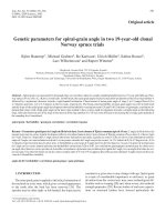
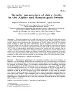
The results obtained with Gibbs sampling are presented in Tables IV and V
and marginal posterior distributions are depicted in Figures 1 and 2. The burn-

in periods varied from 5 to 928 samples, so most samples in the chain were kept
for further processing. The final sample size for the different components var-
ied between 321 and 20 000. After thinning, serial correlations between sam-
ples within each chain were at the most 0.10. The values in the final samples
could therefore be considered sufficiently independent.
In the Suffolk, AM and SM yielded similar posterior distributions. Distri-
butions were fairly symmetric with the mean, mode and median close to each
other and they appeared close to normal. The posterior mean of the heritabil-
ity of litter size was 0.10 and 0.08 for LSN and 0.11 and 0.10 for LSI in AM
and SM respectively. The PE-effect accounted for about 0.06 to 0.09 of the
variance and the YF-effect for 0.05 to 0.06.
Genetic parameters of litter size in sheep 551
Table III. REML estimates for the heritability (h
2
), fraction of the permanent environ-
mental effect (PE
2
) and genetic (r
g
) and environmental correlation (r
pe
) for litter size
after natural oestrus (LSN) and litter size after induced oestrus (LSI) in the Suffolk
and Texel. For the different linear models the Akaike Information Criterion (AIC) is
given, standard errors are given between brackets.
Breed / parameter Model
Suffolk I II III IV Rescaled*
LSN
h
2

0.06 (0.02) 0.06 (0.01) 0.07 (0.02) 0.07 (0.01) 0.12
PE
2
0.02 (0.02) 0.01 (0.00) - - 0.03
LSI
h
2
0.07 (0.03) 0.07 (0.03) 0.07 (0.03) 0.07 (0.03) 0.16
PE
2
0.01 (0.02) - 0.00 (0.02) - -
(LSN,LSI)
r
g
0.57 (0.31) 0.64 (0.28) 0.59 (0.27) 0.59 (0.26) -
r
pe
1.26 (0.00) - - - -
AIC 7758 7755 7756 7755
Texel
LSN
h
2
0.09 (0.01) 0.10(0.01) 0.13 (0.01) 0.13 (0.01) 0.17
PE
2
0.05 (0.01) 0.05 (0.01) - - 0.08
LSI
h
2

0.06 (0.01) 0.08 (0.01) 0.07 (0.01) 0.08 (0.01) 0.13
PE
2
0.03 (0.01) - 0.03 (0.01) - 0.07
(LSN,LSI)
r
g
0.75 (0.10) 0.80 (0.07) 0.81 (0.08) 0.75 (0.06) -
r
pe
0.72 (0.23) - - - -
AIC 57792 57797 57810 57811 -
* Rescaled parameters are presented for model I in Texel and model II in Suffolk.
In the Texel, posterior distributions appeared close to normal. The differ-
ences were noted between AM and SM for the location parameters. In the
AM, the posterior mean of the heritability of litter size was 0.18 for LSN and
0.11 for LSI. In the SM, corresponding values for the heritability were 0.07
and 0.05. The posterior means for the proportion of variance of the PE-effect
were 0.06 and 0.16 for LSN and 0.05 and 0.10 for LSI in AM and SM respec-
tively. For the YF-effects, the means of the posterior distribution ranged from
0.05 to 0.08 and there was no difference between AM and SM.
552 S. Janssens et al.
Table IV. Marginal posterior location parameters (mean, mode, median and standard
deviation) and final sample characteristics (burn in, sample size (N) and serial correla-
tion (corr)) for the heritability (h
2
), variance fraction of the permanent environmental
effect (PE
2
), variance fraction of the year*flock effect (YF

2
) and genetic (r
g
), perma-
nent environmental correlation (r
pe
), year*flock correlation (r
yf
) for litter size after
natural oestrus (LSN) and litter size after induced oestrus (LSI) in the Suffolk.
Parameter Mean Mode Median Std. dev. Burn in N Corr.
Animal model
LSN
h
2
0.10 0.10 0.10 0.02 215 2564 0.06
PE
2
0.06 0.06 0.06 0.01 81 4546 0.00
YF
2
0.06 0.05 0.06 0.01 5 13514 0.03
LSI
h
2
0.11 0.11 0.11 0.03 71 1495 0.07
PE
2
0.07 0.06 0.07 0.02 128 2427 0.02
YF

2
0.06 0.05 0.06 0.02 25 6667 0.00
(LSN,LSI)
r
g
0.44 0.47 0.44 0.13 230 1825 0.02
r
pe
0.40 0.41 0.40 0.17 28 3449 0.03
r
yf
0.33 0.36 0.34 0.17 5 6803 0.03
Sire model
LSN
h
2
0.08 0.08 0.08 0.01 47 20000 0.01
PE
2
0.09 0.09 0.09 0.02 63 5406 0.03
YF
2
0.05 0.05 0.05 0.01 29 13158 0.00
LSI
h
2
0.10 0.09 0.10 0.03 9 10639 0.02
PE
2
0.09 0.08 0.08 0.03 214 2865 0.05

YF
2
0.06 0.05 0.06 0.02 20 6850 0.00
(LSN,LSI)
r
g
0.40 0.45 0.41 0.13 5 14706 0.02
r
pe
0.50 0.56 0.52 0.15 134 3003 –0.01
r
yf
0.33 0.40 0.34 0.17 71 8474 0.01
The posterior means of the genetic correlation between LSN and LSI, were
0.44(AM)and0.40(SM)intheSuffolk and 0.72 (AM) and 0.56 (SM) in
the Texel (Figs. 1 and 2). The mean of the distribution of the correlation be-
tween PE-effects was 0.41 (AM) and 0.50 (SM) in the Suffolk and 0.44 (AM)
Genetic parameters of litter size in sheep 553
Table V. Marginal posterior location parameters (mean, mode, median and standard
deviation) and final sample characteristics (burn in, sample size (N) and serial correla-
tion (corr)) for the heritability (h
2
), variance fraction of the permanent environmental
effect (PE
2
), variance fraction of the year*flock effect (YF
2
) and genetic (r
g
), perma-

nent environmental correlation (r
pe
), year*flock correlation (r
yf
) for litter size after
natural oestrus (LSN) and litter size after induced oestrus (LSI) in the Texel.
Parameter Mean Mode Median Std. dev. Burn in N Corr.
Animal model
LSN
h
2
0.18 0.18 0.17 0.01 69 675 0.07
PE
2
0.06 0.06 0.06 0.01 928 629 0.10
YF
2
0.07 0.07 0.07 0.01 32 4762 0.01
LSI
h
2
0.11 0.11 0.11 0.01 600 424 0.10
PE
2
0.05 0.05 0.05 0.01 391 444 0.09
YF
2
0.05 0.05 0.05 0.01 164 2666 0.01
(LSN, LSI)
r

g
0.72 0.73 0.72 0.05 858 321 0.06
r
pe
0.44 0.47 0.46 0.13 388 475 0.07
r
yf
0.43 0.39 0.43 0.10 102 2511 0.02
Sire model
LSN
h
2
0.07 0.07 0.07 0.01 34 4808 0.04
PE
2
0.16 0.16 0.16 0.01 69 1961 0.02
YF
2
0.08 0.08 0.08 0.01 8 6579 -0.01
LSI
h
2
0.05 0.05 0.05 0.01 242 3011 0.04
PE
2
0.10 0.10 0.10 0.01 23 658 0.04
YF
2
0.06 0.05 0.06 0.01 33 3817 0.02
(LSN, LSI)

r
g
0.56 0.56 0.56 0.07 136 3048 0.03
r
pe
0.72 0.72 0.72 0.07 443 354 0.07
r
yf
0.47 0.48 0.48 0.10 84 2155 0.01
and 0.72 (SM) in the Texel. Corresponding values for the YF*effect were
0.33 (AM) and 0.33 (SM) in the Suffolk and 0.43 (AM) and 0.47 (SM) in
the Texel.
Posterior standard deviations on the variance fractions (i.e. heritability, pro-
portion of the PE-effect, proportion of the YF effect) were between 0.01
and 0.03. For the correlations, the order of magnitude of the standard devi-
ations was between 0.05 and 0.17.
554 S. Janssens et al.
(a)
(b)
Figure 1. Marginal posterior distribution of the genetic correlation between natural
and induced litter size in Suffolk sheep, animal model (a) and sire model (b).
Genetic parameters of litter size in sheep 555
(a)
(b)
Figure 2. Marginal posterior distribution of the genetic correlation between natural
and induced litter size in Texel sheep animal model (a) and sire model (b).
556 S. Janssens et al.
Figure 3. Cumulative percentage of sires for the number of year*flocks per sire
(Suffolk).

Figure 4. Cumulative percentage of sires for the number of year*flocks per sire
(Texel).
4. DISCUSSION
4.1. Data issues
Both the quality of field data and the distribution of effects over animals can-
not be controlled. Imbalance in the data and/or disconnectedness may cause
biased estimates. In order to minimise the risk of bias, data were edited and
Genetic parameters of litter size in sheep 557
“sparse cells” were removed from the dataset. From Figures 3 and 4, the cu-
mulative % of sires appearing in 1, 2, 3, to n different YF-effects, can be eval-
uated. The percentage of sires appearing in only one YF-effect is 10.2% for
LSN and 37% for LSI in the Suffolk. In the Texel breed, these percentages
are respectively 12.4% and 30%. This indicates that most sires are represented
in at least 2 YF-effects. In the Suffolk, one sire had observations on LSN in
44 different YF-effects. In the Texel, the highest count of YF-effects for one
sire was 166. The distribution of sires over YF-effects could be interpreted as
a minimal evaluation of the genetic connectedness. Also the genetic relation-
ships between ewes and between ewes and rams will contribute to the genetic
links.
4.2. Modelling issues
In the preliminary least squares analysis, about 20 to 30% of the variation
in litter size could be attributed to different explanatory variables. The lowest
coefficient of variation was obtained in the Suffolk and for the LSI trait. This
set was the most limited in terms of the number of records and this might ex-
plain the poorer modelling. There is probably scope for improvement of the
model by including other explanatory variables. The preceding litter size (at
birth or at weaning), the weaning to mating interval or a variable describing
the body condition of the ewe could possibly explain non-genetic variation.

However, this information is currently not recorded by the NAMSB and an
extension of the current data collection system in the flock book will be nec-
essary. This extension is only advisable if the extra information can reduce the
residual variance in the model which would result in a higher heritability and
more genetic improvement.
The increase of the mean and the variance of litter size due to hormonal
treatment is also noted in most of the French sheep breeds [3] and in Rasa
Aragonesa sheep [1]. An adverse effect of hormonal treatment on LS has
been found with a reduction of average LS only in prolific breeds, such as
the Romanov, Bleu du Maine, the Flemish breed and in Flemish × Texel-
crosses [3,5]. However, the effects of oestrus induction on LS found in our data
might be slightly biased due to the following reasons: firstly, the ewes were not
randomly assigned to oestrus induction. In Suffolk and Texel, the ewes treated
with hormones before AI or planned matings were probably “preselected” on
general appearance and this could have been a disturbing effect. Secondly, the
ewes returning on induced oestrus cannot be distinguished (in our data) from
ewes mated after normal, i.e. natural oestrus. The ewes returning on induced
558 S. Janssens et al.
oestrus were included as “natural” but an impact of the hormonal treatment on
the next fertilising cycle cannot be excluded. We think, however, that the dis-
turbing effects are limited and that the data were sufficiently good for genetic
parameter estimation.
The separation of the random PE-effect from the residual term is most crit-
ical for LSI because on average, only 1.45 (S) and 1.57 (T) records per ewe
for LSI were available (i.e. 1124 records by 774 ewes in S and 12 550 records
by 7972 ewes in T). For LSN, 2.28 (S) and 1.95 (T) litters per ewe were avail-
able (3885 records by 1701 ewes in S and 27 265 records by 14 009 ewes in T)
which makes the separation of the PE-effect from the residual term feasible.
With REML-techniques, almost no variance was attributed to the PE-effect,
especially for LSI in S. Although S and T do not differ so much in the number

of records per trait, per ewe, differences in the amount of genetic covariance
between animals and in pedigree depth may also have affected the separation
of variance in different components. In S, less daughters per sire were present
than in T (on average 7.9 versus 9.7 ewes/sire) and also pedigree depth was
lower in S as compared to T (3.5 versus 6 generations of known ancestors
on average). The dataset properties mentioned above might explain why the
“best” REML-model was different in S and T.
In the initial Markov chains, burn-in periods were of variable length but con-
siderably shorter than in other studies where up to 5000 and 10 000 samples
were discarded [1, 28]. A flexible choice of the burn-in period is indicated to
save samples. Initial serial correlations between samples were high, indicating
that samples were strongly autocorrelated. The usage of data augmentation is
known to increase auto-correlation in the chain [23] so that more wastage of
samples occurs. In general, final sample sizes were smaller in the runs involv-
ing animal models compared to sire models. Another difference was seen for
posterior distributions involving the PE-effect. In the sire models, the smallest
samples were obtained for chains involving one or both PE-effects. This might
indicate a higher autocorrelation of the Gibbs samples for the permanent en-
vironmental effects than for the genetic or the year*flock effect. In the animal
models, chains involving genetic effects were more autocorrelated and resulted
in smaller final samples for the heritabilities and genetic correlations.
Simulation studies with threshold sire and animal models [15] indicated
convergence problems in the animal models and this was related to the extreme
category problem. Convergence problems were not encountered in our analy-
ses, possibly as the result of treating the YF-effect as random [12,15]. Also the
proportion of YF-effects with a zero variance was restricted in our data (2% in
S and 6% in T) so that the impact of extreme categories was limited.
Genetic parameters of litter size in sheep 559
4.3. Genetic parameters
A mean value of 0.07 for h

2
(LSN) in sheep can be computed from REML-
estimates published before 1995 [8]. Recent REML-estimates for litter size in
sheep ranged from 0.05 to 0.26 [4, 7, 11, 14, 16, 17]. Our REML heritability
estimates for LSN are in agreement with these studies. Heritability estimates
for LSI in Lacaune ewe lambs were 0.05 and 0.06 in two datasets with 1328
and 2201 records, respectively. Only the last estimate was significantly differ-
ent from zero [2] and this value corresponds well with our REML-estimates of
the heritability of LSI in S and T.
In Suffolk, rescaled REML-estimates are higher than the posterior mean ob-
tained with GS whereas in Texel there is good agreement between the rescaled
REML-estimates and posterior means or modes obtained with GS.
Posterior heritabilities obtained with the Gibbs sampler in AM for Suffolk
were close to the posterior mean of 0.08 reported in Rasa Aragonesa sheep [1].
The corresponding Texel results were above this value. GS-results in SM in this
study were lower than the posterior heritabilities for litter size (0.26) in Sabi
sheep [16] and in Baluchi sheep evaluated at three ages (0.34 to 0.43) [28]. In
the latter study, no PE-effect was fitted which is different from our model.
Variance proportions of the PE-effect of litter size are usually small and
in the range of 0.01 to 0.03 [4, 17]. Also in our REML analyses, very little
variance was attributed to the permanent environmental effect whereas with
GS, the distribution of the PE-proportions had a mean between 0.05 and 0.16.
Also, more variance was attributed to PE-effectsinSMascomparedtoAM
and this was seen in both breeds.
The genetic correlation estimates between LSN and LSI obtained with
REML (0.57 to 0.81), were above the value of 0.39 reported in Lacaune ewe
lambs using a sire model [2]. Genetic correlations obtained with SM and GS
corresponded well with the results obtained by Bodin [2].
The differences in genetic correlation estimates found in this study were
partly due to the use of an animal versus a sire model. But, breed differences

might also exist. In prolific breeds, hormonal induction is known to depress
average LS while increasing its variance and this might lead to differences in
genetic correlation estimates between breeds. The moderate to high genetic
correlation, but different from unity, implies that the two types of litter size
should be considered as different traits. Possibly, different sets of genes are in
play. Another reason for the genetic correlation being different from one might
be that insufficient information is provided by the data.
The REML PE-correlation estimate has a large standard error. From the
GS results, it is clear that the PE-correlation was difficult to assess accurately.
560 S. Janssens et al.
Final sample size of the PE-effect was smaller than for the YF or genetic ef-
fect, indicating a slower mixing of the chain. Slower mixing of the chain is
caused by less information coming from the data. In the case of the covariance
between PE-effects, information has to come from subsequent observations of
the two traits in the same animal. Only 26% (S) and 28% (T) of the ewes have
records for both types of oestrus, which means that the within-animal covari-
ance is difficult to estimate and larger standard errors on the covariances and
correlations can be expected.
5. IMPLICATIONS
The magnitude of the heritabilities (0.08 to 0.18 for LSN and 0.05 to 0.11 for
LSI) indicate that genetic improvement of litter size is achievable. Usage of a
threshold model will have an advantage over the use of a linear model because
the heritabilities in the threshold models were higher than in the linear model.
Accounting for the categorical nature of litter size is thus recommended.
A moderately high and positive genetic correlation between natural and in-
duced litter size was found in both breeds and values ranged from 0.40 to 0.81.
Selection for higher (natural) litter size can also be based on observations of
LSI, but progress will be slower. Although natural oestrus is more “informa-
tive” about litter size than induced oestrus, the latter technique is needed to
apply AI or planned matings. These reproductive techniques allow the spread

of the best genes in the population and provide genetic links in the data. Not
discarding the litters after oestrus induction, but including them as a correlated
trait, makes the best use of the information. This can be achieved by imple-
menting a bivariate threshold model for litter size in the Belgian Suffolk and
Texel.
ACKNOWLEDGEMENTS
The Federal Ministry of Agriculture, Medium and Small Enterprises, DG6
– Research and Development, provided funding for conducting this study. The
National Association of Meat Sheep Breeders is acknowledged for supplying
the data.
REFERENCES
[1] Altaribba J., Varona L., Garcia-Cortes L.A., Moreno C., Bayesian inference of
variance components for litter size in Rasa Aragonesa sheep, J. Anim. Sci. 76
(1998) 23–28.
Genetic parameters of litter size in sheep 561
[2] Bodin L., Estimation of genetic parameters of the Lacaune ewe lamb litter size
after fecundation on natural and induced oestrus, Ann. Génét. Sél. Anim. 11
(1979) 413–424.
[3] Bodin L., Elsen J.M., Variability of litter size in French sheep following natural
or induced ovulation, Anim. Prod. 48 (1989) 535–541.
[4] Bromley C.M., van Vleck L.D., Snowder G.D., Genetic correlations for litter
weight weaned with growth, prolificacy, and wool traits in Columbia, Polypay,
Rambouillet and Targhee sheep, J. Anim. Sci. 79 (2001) 339–346.
[5] Calus A.C., Mogelijkheden van intensieve schapenhouderij. Possibilities of in-
tensive sheep breeding, Thesis Geaggregeerde hoger onderwijs, State University
Ghent, Belgium, 1988.
[6] Cameron N.C., Selection indices and prediction of genetic merit in animal breed-
ing, CAB International Wallingford, UK, 1997.
[7] El Fadili M., Leroy P.L., Estimation of additive and non-additive genetic parame-
ters for reproduction, growth and survival traits in crosses between the Moroccan

D’man and Timadhite sheep breed, J. Anim. Breed. Genet. 118 (2001) 341–353.
[8] Fogarty N.M., Genetic parameters for live weight, fat and muscle measurements,
wool production and reproduction in sheep: a review, Anim. Breed. Abstr. 63
(1995) 101–143.
[9] Gianola D., Theory and analysis of threshold characters, J. Anim. Sci. 54 (1982)
1079–1096.
[10] Groeneveld E., VCE4 User’s Guide and Reference Manual, Version 1.3, Institute
of Animal Science, Federal Agricultural Research Center (FAL), Mariensee,
Neustadt, Germany, 1998.
[11] Hagger C., Genetic and environmental influences on size of first litter in sheep,
estimated by the REML method, J. Anim. Breed. Genet. 117 (2000) 57–64.
[12] Hoeschele I., Tier B., Estimation of variance components of threshold characters
by marginal posterior modes and means via Gibbs sampling, Genet. Sel. Evol.
27 (1995) 519–540.
[13] Konstantinov K.V., Erasmus G.J., van Wyk J.B., Evaluation of Dormer sires for
litter size and lamb mortality using a threshold model, S. Afr. J. Anim. Sci. 24
(1998) 119–121.
[14] Lee J.W., Waldron D.F., van Vleck L.D., Parameter estimates for number of
lambs born at different ages and for 18-monthbody weight of Rambouillet sheep,
J. Anim. Sci. 78 (2000) 2086–2090.
[15] Luo M.F., Boettcher P.J., Schaeffer L.R., Dekkers J.C.M., Bayesian inference for
categorical traits with an application to variance component estimation, J. Dairy
Sci. 84 (2001) 694–704.
[16] Matika O., van Wyk J.B., Erasmus G.J., Baker R.L., Genetic parameters in Sabi
sheep, Livest. Prod. Sci. 79 (2003) 17–28.
[17] Matos C.A.P., Thomas D.L., Gianola D., Tempelman R.J., Young L.D., Genetic
analysis of discrete reproductive traits in sheep using linear and nonlinear mod-
els: I. Estimation of genetic parameters, J. Anim. Sci. 75 (1997) 76–87.
[18] Neumaier A., Groeneveld E., Restricted maximum likelihood estimation of co-
variances in sparse linear models, Genet. Sel. Evol. 30 (1998) 3–26.

562 S. Janssens et al.
[19] Olesen I., Perez-Enciso M., Gianola D., Thomas D.L., A comparison of normal
and non-normal mixed models for number of lambs born in Norwegian sheep, J.
Anim. Sci. 72 (1994) 1166–1173.
[20] Olesen I., Svendsen M., Klemetsedal G., Steine T., Application of a multiple-
trait animal model for genetic evaluation of maternal and lamb traits in
Norwegian sheep, Anim. Sci. 60 (1995) 457–469.
[21] SAS


Institute, SAS/S TAT U se r’s Man ua l, Ve rsio n 6, Cary, North Carolina,
United States of America, 1996.
[22] Shaat I., Galal S., Mansour H., Genetic trends for lamb weights in flocks of
Egyptian Rahmani and Ossimi sheep, Small Rumin. Res. 51 (2004) 23–28.
[23] Sorensen D., Gibbs sampling in quantitative genetics, Internal report n
◦
82,
Danish Institute of Agricultural Sciences, 1999.
[24] Van Kaam J.B.C.H.M., Gibanal. Analyzing program for Markov chain Monte
Carlo sequences, Department of Animal Breeding, Wageningen Agricultural
University, The Netherlands, 1998.
[25] Van Tassell C.P., van Vleck L.D., Multiple Trait Gibbs Sampler for Animal
Models: Flexible Programs for Bayesian and Likelihood-Based (Co)Variance
Component Inference, J. Anim. Sci. 74 (1996) 2586–2597.
[26] Van Tassell C.P., van Vleck L.D., Gregory K.E., Bayesian analysis of Twinning
and Ovulation rates using a multiple-trait threshold model and Gibbs sampling,
J. Anim. Sci. 76 (1998) 2048–2061.
[27] Wada Y., Kashiwagi N., Selecting statistical models with information statistics,
J. Dairy Sci. 73 (1990) 3575–3582.
[28] Yazdi M.H., Johansson K., Gates P., Näsholm A., Jorjani H., Liljedahl L E.,

Bayesian analysis of birth weight and litter size in Baluchi sheep using Gibbs
sampling, J. Anim. Sci. 77 (1999) 533–540.
To access this journal online:
www.edpsciences.org