Báo cáo sinh học: " Interval mapping of quantitative trait loci with selective DNA pooling data" pdf
Bạn đang xem bản rút gọn của tài liệu. Xem và tải ngay bản đầy đủ của tài liệu tại đây (231.23 KB, 25 trang )
Genet. Sel. Evol. 39 (2007) 685–709 Available online at:
c
INRA, EDP Sciences, 2007 www.gse-journal.org
DOI: 10.1051/gse:2007026
Original article
Interval mapping of quantitative trait loci
with selective DNA pooling data
Jing Wang
a,b∗
, Kenneth J. Koehler
b
, Jack C.M. Dekkers
a∗∗
a
Department of Animal Science and Center for Integrated Animal Genomics, Iowa State
University, Ames, Iowa 50011, USA
b
Department of Statistics, Iowa State University, Ames, Iowa 50011, USA
(Received 10 October 2006; accepted 21 May 2007)
Abstract – Selective DNA pooling is an efficient method to identify chromosomal regions that
harbor quantitative trait loci (QTL) by comparing marker allele frequencies in pooled DNA
from phenotypically extreme individuals. Currently used single marker analysis methods can
detect linkage of markers to a QTL but do not provide separate estimates of QTL position and
effect, nor do they utilize the joint information from multiple markers. In this study, two inter-
val mapping methods for analysis of selective DNA pooling data were developed and evaluated.
One was based on least squares regression (LS-pool) and the other on approximate maximum
likelihood (ML-pool). Both methods simultaneously utilize information from multiple markers
and multiple families and can be applied to different family structures (half-sib, F2 cross and
backcross). The results from these two interval mapping methods were compared with results
from single marker analysis by simulation. The results indicate that both LS-pool and ML-pool
provided greater power to detect the QTL than single marker analysis. They also provide sepa-
rate estimates of QTL location and effect. With large family sizes, both LS-pool and ML-pool
provided similar power and estimates of QTL location and effect as selective genotyping. With
small family sizes, however, the LS-pool method resulted in severely biased estimates of QTL
location for distal QTL but this bias was reduced with the ML-pool.
selective DNA pooling / interval mapping / QTL
1. INTRODUCTION
Detecting genes underlying quantitative variation (quantitative trait loci or
QTL) with the aid of molecular genetic markers is an important research area
in both animal and plant breeding. However, for QTL with small or moderate
effect, much genotyping is required to achieve a desired power [9] and the
genotyping cost can be prohibitive.
∗
Present address: Pioneer Hi-Bred International, Johnston, Iowa 50131, USA.
∗∗
Corresponding author:
Article published by EDP Sciences and available at
or />686 J. Wang et al.
Selective DNA pooling is an efficient method to detect linkage between
markers and QTL by comparing marker allele frequencies in pooled DNA from
phenotypically extreme individuals [8]. Marker allele frequencies can be esti-
mated by quantifying PCR product in the pool [22] and linkage to a QTL can
be detected by conducting a significance test at each marker. This approach
has been used to detect QTL in dairy cattle [12, 18, 20, 24], beef cattle [13, 26]
and chickens [18, 19, 28].
Analyses of selective DNA pooling data are typically based on single marker
analyses [8], which cannot provide separate estimates of QTL location and
QTL effect, nor can they utilize the joint information from multiple linked
markers around a QTL. Interval mapping methods have been developed to get
around these problems for individual genotyping data [16] but have not been
developed for selective DNA pooling data.
Dekkers [10] showed that pool frequencies for flanking markers contain in-
formation to map a QTL within an interval. In his study, observed marker al-
lele frequencies in the selected DNA pools were modeled as a linear function
of QTL allele frequency in the same pool and recombination rates between
markers, and location and allele frequency of the QTL could then be solved
analytically based on observed frequencies at the two flanking markers. Sim-
ulation results showed that this method provided nearly unbiased estimates
when power was high but was biased when power was low. In addition, es-
timates did not exist for some replicates and others provided estimates out-
side the parameter space. Also, this method is not suitable for pooled analysis
of multiple families and only used data from flanking markers and not from
markers outside the interval [10]. External markers can provide information to
map QTL in the case of DNA pooling data because observed frequencies are
subject to technical errors.
The objective of this study, therefore, was to develop an interval mapping
method to overcome the forementioned problems. Two methods that allow si-
multaneous analysis of selective DNA pooling data from multiple markers and
multiple families were developed. One was based on least squares regression
(LS-pool) and the other on approximate maximum likelihood (ML-pool). Both
methods were evaluated by simulation.
2. MATERIALS AND METHODS
Basic principles of detecting QTL using selective DNA pooling data were
presented by Darvasi and Soller [8]. Figure 1 illustrates its application to a
single half-sib family, with a sire that is heterozygous for a QTL (Qq) and a
Selective DNA pooling QTL mapping 687
p
Q
L
μ
μ
q
μ
μ
Q
q
p
ro
g
en
y
Q progeny
α
f
M
U
(f
m
U
)
p
q
L
p
Q
U
p
q
U
f
M
L
(f
m
L
)
Q
M
q
m
r
sire
μ
U
μ
L
Figure 1. Principles of selective DNA pooling in a sire family, showing the phenotypic
distribution, observed marker allele frequencies ( f
U
M
, f
U
m
and f
L
M
, f
L
m
), and expected
QTL allele frequencies (p
U
Q
, p
U
q
and p
L
Q
, p
L
q
) in the upper (U)andlower(L) phenotypic
tails of progeny from a sire that is heterozygous for a QTL (Qq) and a linked marker
(Mm).
nearby marker (Mm). The sire is mated to multiple dams randomly chosen
from a population in which the marker and QTL are in linkage equilibrium.
In concept, progeny can be separated into two groups, depending on the QTL
allele received from the sire. The dam’s QTL alleles, polygenic effects and
environmental factors contribute to variation within each group of progeny, re-
sulting in normally distributed phenotypes for the quantitative trait within each
group. For selective DNA pooling, progeny are ranked based on phenotype and
the highest and lowest p% are selected. An equal amount of DNA is extracted
from each selected individual and DNA from individuals in the same selected
tail is pooled to form upper and lower pools. The frequency of marker alle-
les in each pool can be determined by densitometric PCR or other quantitative
genotyping methods. Three alternative methods for analysis of the resulting
data will be presented.
688 J. Wang et al.
2.1. Single marker association analysis
This method tests for a difference in allele frequencies between the upper
and lower pools at a given marker, following Darvasi and Soller [8]. With an
approximate normal distribution, the null hypothesis that a marker is not linked
to a QTL is rejected with type I error α if
Z
ij
< Z
α/2
or Z
ij
> Z
1−α/2
,
with Z
ij
=
( f
U
M
ij
+ f
L
m
ij
)
2
− 0.5
Var
⎛
⎜
⎜
⎜
⎜
⎜
⎜
⎝
f
U
M
ij
+ f
L
m
ij
2
⎞
⎟
⎟
⎟
⎟
⎟
⎟
⎠
,
where f
U
M
ij
, f
U
m
ij
, f
L
M
ij
and f
L
m
ij
are the observed frequencies of paternal marker
alleles M and m in the upper (U)andlower(L) pools for the j
th
marker in the
i
th
family, and Z
α/2
and Z
1−α/2
are ordinates of the standard normal distribution
such that the area from –∞ to Z
α/2
or Z
1−α/2
equals α/2or1−α/2, respectively.
Since both sampling errors and technical errors (assumed independent of sam-
pling errors) contribute to deviations of observed allele frequencies from their
expectations, the variance of pool allele frequency under the null hypothesis
can be estimated as [8]:
Var
⎛
⎜
⎜
⎜
⎜
⎜
⎜
⎝
f
U
M
ij
+ f
L
m
ij
2
⎞
⎟
⎟
⎟
⎟
⎟
⎟
⎠
=
1
2
0.25
n
i
+ V
TE
,
where n
i
is the number of individuals per pool for family i,
0.25
n
i
is the variance
of binomial sampling errors under the null hypothesis and V
TE
is the variance
of technical errors associated with estimation of allele frequencies from DNA
pools. Estimates of variance V
TE
could be obtained from previous studies, e.g.,
by comparing pool estimates of marker allele frequencies with the true fre-
quency obtained from individual genotyping. If V
TE
is unknown, the required
variance of allele frequencies can be directly estimated from the available data,
following Lipkin et al. [18]: assuming symmetry, f
U
M
ij
and f
L
m
ij
are expected to
be equal and the only reason for a difference between them is binomial sam-
pling error and technical error. Consequently,
ˆ
Var
⎛
⎜
⎜
⎜
⎜
⎜
⎜
⎝
f
U
M
ij
+ f
L
m
ij
2
⎞
⎟
⎟
⎟
⎟
⎟
⎟
⎠
=
1
4
ˆ
Var
f
U
M
ij
− f
L
m
ij
=
1
4(mk − 1)
m
i=1
k
j=1
f
U
M
ij
− f
L
m
ij
2
,
where m is the number of families and k is the number of markers examined
by selective DNA pooling.
Selective DNA pooling QTL mapping 689
If information from m families is available, the Z-test for each family can
be incorporated into a Chi-square test, assuming that observations from each
family are independent [8]. When several markers are available on a chromo-
some or within a chromosomal region, the marker with the most significant
test statistic is considered to be the marker closest to the QTL.
2.2. Least squares interval mapping (LS-pool)
Consider a chromosome with k markers and a single QTL, with phase and
positions of markers assumed known. Then, following Dekkers [10], the ob-
served frequency of allele M for marker j in the upper and lower pools of
family i ( f
U
M
ij
and f
L
M
ij
) can be modeled in terms of the expected QTL allele
frequency in the same pools for family i (p
U
Q
i
and p
L
Q
i
) and the recombination
rate (r
j
) between marker j and the QTL as follows:
f
U
M
ij
= (1 − r
j
)p
U
Q
i
+ r
j
(1 − p
U
Q
i
) + se
U
ij
+ te
U
ij
,
and f
L
M
ij
= (1 − r
j
)p
L
Q
i
+ r
j
(1 − p
L
Q
i
) + se
L
ij
+ te
L
ij
,
where p
U
Q
i
and p
L
Q
i
are the expected frequencies of the paternal Q allele in the
upper (U)andlower(L) pools in the i
th
family, and se
U
ij
and se
L
ij
, te
U
ij
and te
L
ij
are the sampling and technical errors for marker j in the upper and lower pools
of family i.
Deviating frequencies from their expectation of
1
/
2
under the null hypothesis
of no QTL and replacing p
L
Q
i
with1–p
U
Q
i
, assuming a symmetric distribution
of phenotypes (Fig. 1) and equal selected proportions for both pools, models
can be reformulated as:
f
U
M
ij
− 1/2 = (1 − 2r
j
)(p
U
Q
i
− 1/2) + se
U
ij
+ te
U
ij
,
and f
L
M
ij
− 1/2 = −(1 − 2r
j
)(p
U
Q
i
− 1/2) + se
L
ij
+ te
L
ij
.
Combining equations across k markers results in:
⎡
⎢
⎢
⎢
⎢
⎢
⎢
⎢
⎢
⎢
⎢
⎢
⎢
⎢
⎢
⎢
⎢
⎢
⎢
⎢
⎢
⎢
⎢
⎢
⎢
⎢
⎢
⎢
⎢
⎢
⎢
⎢
⎢
⎢
⎢
⎢
⎢
⎢
⎣
f
U
M
i1
− 1/2
f
U
M
i2
− 1/2
f
U
M
ik
− 1/2
f
L
M
i1
− 1/2
f
L
M
i2
− 1/2
f
L
M
ik
− 1/2
⎤
⎥
⎥
⎥
⎥
⎥
⎥
⎥
⎥
⎥
⎥
⎥
⎥
⎥
⎥
⎥
⎥
⎥
⎥
⎥
⎥
⎥
⎥
⎥
⎥
⎥
⎥
⎥
⎥
⎥
⎥
⎥
⎥
⎥
⎥
⎥
⎥
⎥
⎦
=
⎡
⎢
⎢
⎢
⎢
⎢
⎢
⎢
⎢
⎢
⎢
⎢
⎢
⎢
⎢
⎢
⎢
⎢
⎢
⎢
⎢
⎢
⎢
⎢
⎢
⎢
⎢
⎢
⎢
⎢
⎢
⎢
⎢
⎢
⎢
⎢
⎣
1 − 2r
1
1 − 2r
2
1 − 2r
k
−(1 − 2r
1
)
−(1 − 2r
2
)
−(1 − 2r
k
)
⎤
⎥
⎥
⎥
⎥
⎥
⎥
⎥
⎥
⎥
⎥
⎥
⎥
⎥
⎥
⎥
⎥
⎥
⎥
⎥
⎥
⎥
⎥
⎥
⎥
⎥
⎥
⎥
⎥
⎥
⎥
⎥
⎥
⎥
⎥
⎥
⎦
p
U
Q
i
− 1/2
+
⎡
⎢
⎢
⎢
⎢
⎢
⎢
⎢
⎢
⎢
⎢
⎢
⎢
⎢
⎢
⎢
⎢
⎢
⎢
⎢
⎢
⎢
⎢
⎢
⎢
⎢
⎢
⎢
⎢
⎢
⎢
⎢
⎢
⎢
⎢
⎢
⎣
se
U
i1
se
U
i2
se
U
ik
se
L
i1
se
L
i2
se
L
ik
⎤
⎥
⎥
⎥
⎥
⎥
⎥
⎥
⎥
⎥
⎥
⎥
⎥
⎥
⎥
⎥
⎥
⎥
⎥
⎥
⎥
⎥
⎥
⎥
⎥
⎥
⎥
⎥
⎥
⎥
⎥
⎥
⎥
⎥
⎥
⎥
⎦
+
⎡
⎢
⎢
⎢
⎢
⎢
⎢
⎢
⎢
⎢
⎢
⎢
⎢
⎢
⎢
⎢
⎢
⎢
⎢
⎢
⎢
⎢
⎢
⎢
⎢
⎢
⎢
⎢
⎢
⎢
⎢
⎢
⎢
⎢
⎢
⎢
⎣
te
U
i1
te
U
i2
te
U
ik
te
L
i1
te
L
i2
te
L
ik
⎤
⎥
⎥
⎥
⎥
⎥
⎥
⎥
⎥
⎥
⎥
⎥
⎥
⎥
⎥
⎥
⎥
⎥
⎥
⎥
⎥
⎥
⎥
⎥
⎥
⎥
⎥
⎥
⎥
⎥
⎥
⎥
⎥
⎥
⎥
⎥
⎦
(Model 1),
690 J. Wang et al.
or in matrix notation:
f
i
− 1/2 = X
i
[p
U
Q
i
− 1/2] + se
i
+ te
i
,
where f
i
is a vector with observed marker allele frequencies for family i and
1
/
2
is a vector with elements
1
/
2
. For the least squares analysis, sampling and
technical errors are combined into a single residual vector: e
i
= se
i
+te
i
.
For a given putative position of the QTL, recombination rates r
j
are known
and, thus, elements of matrix X
i
are known, and Model 1 can be fitted using
ordinary least squares:
f
i
− 1/2 = X
i
β
i
+ e
i
.
This model can be extended to multiple independent sire families by simply
expanding the dimensions of the matrices in Model 1. Using a common QTL
position, the multi-family model estimates separate QTL allele frequency de-
viations for each family, which allows for a different QTL substitution effect
for each sire.
Similar to least squares interval mapping with individual genotyping data
[14], the model is fitted at each putative QTL position and ordinary least
squares is used to estimate parameters β
i
= (p
U
Q
i
−
1
/
2
), assuming residuals
are identically and independently distributed. The following test statistics are
calculated at each position and the position with the highest statistic is taken
as the estimate of QTL position:
if V
TE
is known,
χ
2
=
m
i=1
χ
2
i
=
m
i=1
SS
regression,i
Var ( f
M
i
)
H
0
=
m
i=1
(f
i
− 1/2)
X
i
(X
i
X
i
)
−1
X
i
(f
i
− 1/2)
(
0.25
n
i
+ V
TE
)
,
where SS
regression,i
is the sum of squares of regression for family i;
if V
TE
is not known,
F =
m
i=1
SS
regres sion,i
m
m
i=1
SS
error,i
m · (2k − 1)
=
m
i=1
(f
i
− 1/2)
X
i
(X
i
X
i
)
−1
X
i
(f
i
− 1/2)
m
m
i=1
(f
i
− 1/2)
[I − X
i
(X
i
X
i
)
−1
X
i
](f
i
− 1/2)
m · (2k − 1)
,
where SS
error,i
is the sum squares of residuals for family i. Estimated QTL al-
lele frequencies at the best position are then used to estimate QTL substitution
effects for each sire i,
ˆ
α
i
, following Dekkers [10].
In some applications, D values – the difference in observed marker allele fre-
quencies between the upper and lower pools – are used for QTL mapping [17].
Selective DNA pooling QTL mapping 691
To adapt to handle D values, the following model can be used:
⎡
⎢
⎢
⎢
⎢
⎢
⎢
⎢
⎢
⎢
⎢
⎢
⎢
⎢
⎣
D
M
i1
D
M
i2
D
M
ik
⎤
⎥
⎥
⎥
⎥
⎥
⎥
⎥
⎥
⎥
⎥
⎥
⎥
⎥
⎦
=
⎡
⎢
⎢
⎢
⎢
⎢
⎢
⎢
⎢
⎢
⎢
⎢
⎢
⎢
⎣
1 − 2r
1
1 − 2r
2
1 − 2r
k
⎤
⎥
⎥
⎥
⎥
⎥
⎥
⎥
⎥
⎥
⎥
⎥
⎥
⎥
⎦
D
Q
i
+
⎡
⎢
⎢
⎢
⎢
⎢
⎢
⎢
⎢
⎢
⎢
⎢
⎢
⎢
⎣
e
D
i1
e
D
i2
e
D
ik
⎤
⎥
⎥
⎥
⎥
⎥
⎥
⎥
⎥
⎥
⎥
⎥
⎥
⎥
⎦
,
or in matrix notation: D
i
= X
i
D
Q
i
+ e
i
, (Model 2)
where D
M
ij
is the D value of the j
th
marker of the i
th
sire family, D
Q
i
is the
expected D value for the QTL allele of the i
th
sire family, and e
D
ij
are residuals,
including both sampling and technical errors, with variance equal to SE
2
D
ij
,
which can be derived as described in Lipkin et al. [17], accounting for variance
of technical error, the overlap of sire marker alleles with those of its mates,
different numbers of pools and replicates, and different numbers of daughters
per pool. A weighted least squares [23] method can then be applied to allow
for different values of SE
2
D
ij
for different sires. The test statistic, summed over
families at a given putative QTL position, can then be derived as:
χ
2
=
m
i=1
χ
2
D
i
=
m
i=1
D
i
V
−1
i
X
i
(X
i
V
−1
i
X
i
)
−1
X
i
V
−1
i
D
i
,
where V
i
is a diagonal matrix with variances SE
2
D
ij
as elements.
2.3. Approximate maximum likelihood interval mapping
method (ML-pool)
Sampling errors that contribute to observed frequencies at linked markers
for a given family, i.e. elements of vector se
i
in model 1, are correlated. These
correlations are not accounted for by the LS-pool method, which reduces its
efficiency. An approximate maximum likelihood method, ML-pool, was devel-
oped to overcome this problem.
In the ML-pool method, the distribution of e
i
= se
i
+ te
i
is approximated
to multivariate normality, given the multi-factorial nature of technical errors,
near-normality of the distribution of the binomial sampling errors with suf-
ficiently large n
i
(n
i
> 30), and the small probability that modeled frequen-
cies fall outside the parameter space (0–1), since the expected allele frequency
is near 0.5. With the expectation of the vector of marker allele frequencies
for sire i defined as in Model 1 (X
i
β
i
), the covariance matrix is defined as:
Σ
i
=
Σ
U
i
0
0 Σ
L
i
, where matrices Σ
U
i
and Σ
L
i
are the covariance matrices of
692 J. Wang et al.
residuals for marker allele frequencies within the upper and lower pools of
family i. By conditioning on the proportion selected for the upper and lower
pool within a family, marker frequencies from the upper and lower pool are
uncorrelated. Variances and covariances in Σ
U
i
are defined as:
Var (e
U
ij
) = Var( se
U
ij
+ te
U
ij
) = Var ( se
U
ij
) + V
TE
=
p
U
M
ij
(1 − p
U
M
ij
)
n
+ V
TE
.
If markers j and l bracket the QTL (M
j
-Q-M
l
) then:
Cov(e
U
ij
, e
U
il
) = Cov(se
U
ij
+ te
U
ij
, se
U
il
+ te
U
il
) = Cov(se
U
ij
, se
U
il
) =
(1 − 2r
jl
)p
U
Q
i
(1 − p
U
Q
i
)
n
i
,
where r
jl
is the recombination rate between markers (see Appendix online for
detailed derivation).
If the marker order is (M
j
-M
l
-Q):
Cov(e
U
ij
, e
U
il
) =
(1 − 2r
jl
)[(1 − r
l
)p
U
Q
i
+ r
l
(1 − p
U
Q
i
)][1 − (1 − r
l
)p
U
Q
i
− r
l
(1 − p
U
Q
i
)]
n
i
,
assuming p
L
Q
i
= 1–p
U
Q
i
, Σ
L
i
= Σ
U
i
.
Both X
i
β
i
and Σ
i
are functions of p
U
Q
i
and r, the vector of recombination
rates between markers and QTL, which is determined by QTL location. Con-
sequently, for a given QTL location (π
Q
) and certain values of p
U
Q
i
, the like-
lihood function for the vector of observed allele frequencies of k markers for
m independent families, based on approximation to multivariate normality, is:
L(f − 1/2
π
Q
, p
U
Q
) =
m
i=1
L(f
i
− 1/2
π
Q
, p
U
Q
) =
m
i
(2π)
−
k
2
|Σ
i
|
−
1
2
exp[(f
i
− 1/2 − x
i
β
i
)
Σ
−1
i
(f
i
− 1/2 − x
i
β
i
)].
Under the null hypothesis of no QTL, p
U
Q
i
=
1
/
2
for each family and the likeli-
hood is a constant (L
0
(f–
1
/
2
)) and does not depend on QTL location. Under the
alternative hypothesis, the likelihood function (L
A
(f–
1
/
2
)) can be maximized by
a golden-section search algorithm [15] for the optimal p
U
Q
i
of each family at a
given QTL position (π
Q
) and the following log likelihood ratio statistic (LR)
can be calculated
LR(L
Q
, p
U
Q
1
, p
U
Q
2
, ,p
U
Q
m
π
Q
) = ln(
L
o
(f
i
− 1/2)
L
A
(f
i
− 1/2)
).
Selective DNA pooling QTL mapping 693
Each putative QTL position along the chromosome is tested and the set of pa-
rameters (π
Q
and p
U
Q
1
,p
U
Q
2
, , p
U
Q
m
) that provides the highest LR gives the
estimates of QTL position and QTL allele frequencies, which are used to es-
timate QTL allele substitution effects for each sire, as for the LS-pool. With
unknown technical error variance, V
TE
is included as an additional parameter
to be optimized in the search routine.
For D values, the covariance matrix can be adapted by including SE
2
D
ij
on the
diagonal and off-diagonals that are the sum of the covariances for residuals of
observed marker allele frequencies in the upper and lower pools and a similar
likelihood ratio statistic (LR) can be calculated.
2.4. Simulation model and parameters
Ten half-sib families with 500 or 2000 progeny per family were simulated
to validate the proposed methods. The simulated population structure was de-
signed to mimic dairy cattle data used for a selective DNA pooling study by
Lipkin et al. [17] and Mosig et al. [20]. For each individual, six fully informa-
tive markers were evenly spaced on a 100 cM chromosome (including markers
at the ends). Dam alleles were assumed to be different from sire alleles and
in population-wide linkage equilibrium with the QTL. Crossovers were gener-
ated according to the Haldane mapping function, which implies independence
of recombination events in adjacent intervals on the chromosome. A single
additive bi-allelic QTL with population frequency 0.5 was simulated at posi-
tion 11 or 46 cM, with an allele substitution effect of 0.25 phenotypic standard
deviations, which was set equal to 1. Heritability was 0.25 and phenotypic val-
ues of progeny were affected by the QTL along with polygenic effects and
environmental factors, which were both normally distributed, and simulated
as:
y
ij
= μ + g
QT L
ij
+ 1/2 g
sire
i
+ 1/2 g
dam
ij
+ g
M
ij
+ ε
ij
,
where y
ij
is the phenotypic value of progeny j of sire i, μ is the overall mean,
g
QT L
ij
is the QTL effect based on the QTL alleles received from the sire and
dam, g
sire
i
is the polygenic effect of the sire i, g
dam
ij
is the polygenic effect of
dam j mated to sire i, g
M
ij
is the polygenic effect due to Mendelian sampling,
and ε
ij
is the environmental effect for progeny j of sire i. Progeny were ranked
by phenotype within each half-sib family and the top and bottom 10% con-
tributed to DNA pools. For each marker, the true paternal allele frequencies
in pools were obtained by counting and a normally distributed technical error
with mean zero and zero variance (no technical error) or 0.0014 was added.
694 J. Wang et al.
Then, to satisfy the condition that frequencies of the two alleles sum to one,
simulated frequencies were divided by the sum of the simulated frequencies of
the two paternal alleles. The resulting variance due to technical errors in the
observed allele frequencies was either V
TE
= 0.0 or V
TE
= 0.0007. The latter
was equal to the technical error variance estimated by Lipkin et al. [17]. Allele
frequencies were observed for each half-sib family and for all markers.
Single marker analysis, LS-pool and ML-pool were applied to the simu-
lated selective DNA pooling data, with or without previous knowledge about
technical error variance. Sire marker haplotypes were assumed known. For
comparison, the simulated data were also analyzed by selective genotyping
by applying regular least squares interval mapping [14] to individual marker
genotype and phenotype data on individuals with high and low phenotypes.
Estimates of QTL effects were adjusted based on selection intensity following
Darvasi and Soller [8].
For each set of parameters and each mapping method, the criteria for com-
parison of methods were the following: (1) power to detect the QTL, (2) bias
and variance of estimates of QTL location, and (3) bias and variance of esti-
mates of QTL effects. The LS-pool, ML-pool and selective genotyping meth-
ods provide separate estimates of QTL location and QTL effect. For single
marker analyses, position of the most significant marker was used as the esti-
mate of QTL position. For each set of parameters and each mapping method,
10 000 replicates were simulated under the null hypothesis of no QTL to de-
termine 5% chromosome-wise significant thresholds of the test statistics and
3000 replicates were simulated under the alternative hypothesis.
2.5. Validation of the symmetry assumption
One important assumption in both LS-pool and ML-pool is that distribu-
tions of phenotypic values within the group of progeny receiving the “Q” or
“q” allele from the sire are the same and symmetric. Under this assumption,
frequency p
U
Q
i
is expected to be equal to p
L
q
i
and, therefore, only one parameter
for QTL allele frequency needs to be estimated. This symmetry assumption
will be invalid if the QTL is dominant or if the QTL allele frequency among
dams is not 0.5. Under these situations, Qq progeny will not be equally dis-
tributed across the upper and lower pools and it may be more appropriate to fit
two QTL allele frequency parameters in the model, one for each selected pool.
Selective DNA pooling QTL mapping 695
Then Model 1 becomes:
⎡
⎢
⎢
⎢
⎢
⎢
⎢
⎢
⎢
⎢
⎢
⎢
⎢
⎢
⎢
⎢
⎢
⎢
⎢
⎢
⎢
⎢
⎢
⎢
⎢
⎢
⎢
⎢
⎢
⎢
⎢
⎢
⎢
⎢
⎢
⎢
⎢
⎢
⎣
f
U
M
i1
− 1/2
f
U
M
i2
− 1/2
f
U
M
ik
− 1/2
f
L
M
i1
− 1/2
f
L
M
i2
− 1/2
f
L
M
ik
− 1/2
⎤
⎥
⎥
⎥
⎥
⎥
⎥
⎥
⎥
⎥
⎥
⎥
⎥
⎥
⎥
⎥
⎥
⎥
⎥
⎥
⎥
⎥
⎥
⎥
⎥
⎥
⎥
⎥
⎥
⎥
⎥
⎥
⎥
⎥
⎥
⎥
⎥
⎥
⎦
=
⎡
⎢
⎢
⎢
⎢
⎢
⎢
⎢
⎢
⎢
⎢
⎢
⎢
⎢
⎢
⎢
⎢
⎢
⎢
⎢
⎢
⎢
⎢
⎢
⎢
⎢
⎢
⎢
⎢
⎢
⎢
⎢
⎢
⎢
⎢
⎢
⎣
1 − 2r
1
0
1 − 2r
2
0
0
1 − 2r
k
0
01− 2r
1
01− 2r
2
0
01− 2r
k
⎤
⎥
⎥
⎥
⎥
⎥
⎥
⎥
⎥
⎥
⎥
⎥
⎥
⎥
⎥
⎥
⎥
⎥
⎥
⎥
⎥
⎥
⎥
⎥
⎥
⎥
⎥
⎥
⎥
⎥
⎥
⎥
⎥
⎥
⎥
⎥
⎦
p
U
Q
i
− 1/2
p
L
Q
i
− 1/2
+
⎡
⎢
⎢
⎢
⎢
⎢
⎢
⎢
⎢
⎢
⎢
⎢
⎢
⎢
⎢
⎢
⎢
⎢
⎢
⎢
⎢
⎢
⎢
⎢
⎢
⎢
⎢
⎢
⎢
⎢
⎢
⎢
⎢
⎢
⎢
⎢
⎣
e
U
i1
e
U
i2
e
U
ik
e
L
i1
e
L
i2
e
L
ik
⎤
⎥
⎥
⎥
⎥
⎥
⎥
⎥
⎥
⎥
⎥
⎥
⎥
⎥
⎥
⎥
⎥
⎥
⎥
⎥
⎥
⎥
⎥
⎥
⎥
⎥
⎥
⎥
⎥
⎥
⎥
⎥
⎥
⎥
⎥
⎥
⎦
(Model 3).
The symmetry assumption was evaluated and results from least squares models
that fitted one (LS-pool-1) or two QTL frequencies (LS-pool-2), one for the
upper and one for the lower pool, were compared for different combinations of
QTL dominance and QTL allele frequencies among dams. Since the ML-pool
is computationally more demanding and the difference between the LS-pool
and ML-pool was not expected to be large, only LS-pool was investigated.
3. RESULTS
3.1. Comparison of QTL mapping results
3.1.1. Power
Table I shows power for the LS-pool, ML-pool and single marker methods
of analysis of the simulated selective DNA pooling data and of selective geno-
typing analysis of the simulated individual genotyping data. All four methods
resulted in high and similar power (97%) for the large family size and mod-
erate power (51 to 80%) with small family size (Tab. I). Power was the highest
for selective genotyping, because it is not affected by technical errors associ-
ated with pooling and utilizes the distribution of phenotypes within the pheno-
typic tails. Power for selective genotyping was, however, only up to 6% greater
than for the ML-pool. Among methods using selective DNA pooling data, for
most situations, ML-pool provided the highest power, followed by LS-pool
and single marker analysis. The power of the LS-pool was, however, signif-
icantly affected by true QTL position, and was close to or lower than power
from single marker analysis for non-central QTL, and similar to or greater than
power from the ML-pool for central QTL with known V
TE
. For the latter case,
power from the LS-pool was even greater than power from selective genotyp-
ing. These discrepancies resulted from the heterogeneous distribution of the
696 J. Wang et al.
Tabl e I. Power (%) to detect the QTL from analysis of selective DNA pooling data by
least squares (LS-pool), maximum likelihood (ML-pool) and single marker analysis,
and of least squares analysis with selective genotyping data.
Family V
TE
True QTL Selective DNA pooling Selective
size (×10
4
) location LS-pool ML-pool Single marker genotyping
V
TE
un/known V
TE
un/known V
TE
un/known
500
7
11 56 / 67 72 / 72 51 / 67 78
46 70 / 78 73 / 73 55 / 72 79
0
11 57 / 70 74 / 75 54 / 74 78
46 70 / 80 77 / 77 57 / 76 79
2000
7
11 97 / 98 99 / 99 94 / 98 100
46 99 / 99 99 / 99 96 / 98 100
0
11 98 / 99 99 / 100 98 / 99 100
46 99 / 99 99 / 100 98 / 99 100
Variance of technical errors from pooling (V
TE
) was unknown or known. There were 10 half-sib
families with 500 or 2000 progeny and the QTL effect was 0.25 phenotypic standard devia-
tions at 11 or 46 cM on a 100 cM chromosome with six equidistant fully informative markers.
The selected proportion was 10% in each pool and V
TE
was 0.0007 or 0. The results of selec-
tive genotyping were independent of V
TE
and are presented twice. The results were based on
3000 replicates and 5% chromosome-wise thresholds were obtained from 10 000 replicates of
simulation under the null hypothesis.
test statistic used for the LS-pool, as demonstrated in Figure 2, which shows
the mean and variance of the test statistic under the null hypothesis at each
putative QTL position for the LS-pool, ML-pool, and selective genotyping,
with small family size (500 progeny) and unknown V
TE
of 0.0007. Both mean
and variance of the F statistic were greater at positions around the center of
the chromosome for the LS-pool, but similar across positions for the ML-pool
and selective genotyping methods. This heterogeneous distribution of the test
statistic causes power to detect the QTL to be overestimated for central QTL
and to be underestimated for distal QTL, since a uniform significance thresh-
old was applied. The heterogeneous distribution of the test statistic, which is
unique to the LS-pool method, is caused by the fact that the LS-pool uses
information from all markers simultaneously but does not account for corre-
lations in frequencies between linked markers. This results in a greater mean
and variance of the test statistic at central positions under the null hypothesis
for the LS-pool, where more marker data are available in the neighborhood of
the evaluated position, than at the ends of the chromosome.
Incorporating previous knowledge of V
TE
in the analysis resulted in 16 to
21% greater power for single marker analysis and 8 to 13% greater power
for the LS-pool but had a limited impact on power for the ML-pool (Tab. I,
Selective DNA pooling QTL mapping 697
0
1
2
3
4
5
6
7
020406080100
Position
F or LR statistic
average of F of LS-pool
variance of F of LS-pool
average of LR of ML-pool variance of LR of ML-pool
average of F of selective genotying
variance of F of selective genotyping
Figure 2. Mean and variance of the test statistic at each possible QTL position for
the LS-pool, ML-pool and selective genotyping methods under the null hypothesis of
no QTL. Ten half-sib families with 500 progeny were used. The variance of technical
errors from pooling was 0.0007 and assumed unknown. The results were based on
100 000 replicates for LS-pool and ML-pool and 10 000 replicates for the selective
genotyping method. Other simulation parameters were the same as in Table III.
small family size). Power of the LS-pool was 10 to 14% greater for a central
QTL than for a distal QTL, 2 to 5% greater for single marker analysis, but
only 1 to 2% greater for the ML-pool. The presence of technical errors (V
TE
=
0.0007 versus 0) only slightly decreased power (5%) for all methods and in
all situations, except that single marker analysis with known V
TE
and a distal
QTL had 7% greater power when no technical errors were present.
3.1.2. Estimates of QTL position
Table II shows means and standard errors (as a measure of mapping accu-
racy) of estimates of QTL location obtained from the four methods. The results
698 J. Wang et al.
Table II. Means and standard errors (in brackets) of estimates of QTL location (in cM)
from analysis of selective DNA pooling data by least squares (LS-pool), maximum
likelihood (ML-pool) and single marker analysis, and of least squares analysis of se-
lective genotyping data.
Family V
TE
QTL Selective DNA pooling Selective
size (×10
4
) location LS-pool ML-pool Single marker genotyping
500 7 11 21.1 (16.7) 18.0 (19.9) 18.4 (21.3) 15.8 (16.2)
46 46.6 (12.1) 45.6 (16.2) 45.7 (18.1) 45.6 (14.3)
0 11 20.4 (15.1) 16.8 (17.6) 16.7 (19.2) 15.8 (16.2)
46 46.5 (11.1) 45.2 (14.8) 45.1 (16.6) 45.6 (14.3)
2000 7 11 13.4 (7.7) 12.0 (7.1) 12.5 (11.9) 11.2 (4.0)
46 45.8 (5.7) 45.3 (6.7) 43.6 (9.6) 45.7 (4.3)
0 11 12.8 (5.9) 11.3 (4.3) 13.0 (10.4) 11.2 (4.0)
46 45.9 (4.5) 45.4 (4.6) 41.5 (6.0) 45.7 (4.3)
The results are for known technical error variance (V
TE
) but were almost the same with un-
known V
TE
. The results of selective genotyping were independent of V
TE
and are presented
twice. The results were based on 3000 replicates. Other simulation parameters are as in Ta-
ble I.
were little affected by prior knowledge of technical error variance, so only re-
sults with known variance are shown. With a central QTL or with large family
size, all four methods resulted in nearly unbiased estimates of QTL location
(bias 4.5 cM) but with distal QTL and small family size, all four methods
resulted in some bias toward the center of the chromosome. Biases were the
smallest for selective genotyping (<5 cM) and the greatest for the LS-pool (9 to
11 cM). Estimates from the ML-pool had similar biases as single marker anal-
ysis (6 to 8 cM). The presence of technical errors only slightly increased biases
(<2 cM) for all situations and with all four methods. Standard errors (SE) of
estimates of QTL location were reasonable with large family size (<12 cM)
but large (11 to 21 cM) with small family size for all four methods. Standard
errors were up to 4.6 cM larger for distal than central QTL and the presence
of technical errors increased SE’s by 1 to 3.6 cM. Single marker analysis had
location estimates with the largest SE. With large family size, selective geno-
typing had smaller SE of location estimates than other methods. But with small
family size, the LS-pool had the smallest SE, even smaller than selective geno-
typing, except for distal QTL and with the presence of technical errors. This
result is also caused by the heterogeneous distribution of the test statistic for
the LS-pool, which results in a tendency of higher test statistics around the cen-
ter of the chromosome (Fig. 2) and, therefore, regression of position estimates
towards the center.
Selective DNA pooling QTL mapping 699
Table III. Means and standard errors (in brackets) of estimates of location (in cM) for
significant (5% chromosome-wise level) QTL from analysis of selective DNA pooling
data by least squares (LS-pool), maximum likelihood (ML-pool) and single marker
analysis, and of least squares analysis of selective genotyping data.
Family V
TE
QTL Selective DNA pooling Selective
size (×10
4
) location LS-pool ML-pool Single marker genotyping
500 7 11 20.1 (13.2) 14.7 (13.9) 14.8 (15.8) 13.6 (11.3)
46 46.6 (12.1) 45.5 (13.1) 45.0 (14.7) 45.5 (11.6)
0 11 19.7 (11.9) 14.0 (11.6) 13.8 (13.6) 13.6 (11.3)
46 46.1 (9.4) 45.1 (11.9) 44.0 (13.2) 45.5 (11.6)
Only QTL location estimates with known variance of technical errors (V
TE
) are presented as
an example. The results of selective genotyping were independent of V
TE
and are presented
twice. Other simulation parameters were the same as Table I, except that only results with
500 progeny were presented.
3.1.3. Estimates of QT L effects
Only interval mapping methods (LS-pool, ML-pool and selective geno-
typing methods) provide estimates of QTL effects. Single marker analy-
sis does provide estimates of marker-associated effects but these were not
evaluated. All methods gave unbiased or nearly unbiased estimates of QTL
effects and similar SE’s of estimates (results not shown). Means and ac-
curacy of estimates of QTL effects with known or unknown technical er-
rors were essentially the same for the LS-pool and ML-pool. Standard er-
rors were small (0.06–0.07 phenotypic standard deviations) for large families
(2000 progeny) but were doubled (0.13 to 0.14 standard deviations) for small
families (500 progeny). The ratio of SE of estimates of QTL effects was pro-
portional to the square root of the ratio family size, as expected for estimates
from regular linear regression. True QTL location and the presence of technical
error had little effect on estimates of QTL effects.
3.1.4. Comparison of methods based on significant replicates
Generally, only significant QTL mapping results are reported from actual
experiments. Thus, it is also necessary to evaluate methods based on significant
replicates only. Table III shows means and SE’s of estimates of QTL location
based on only significant replicates for the small family size (all methods had
high power with large family size, so the results were almost unchanged with
only significant replicates and therefore omitted). The results with known and
unknown V
TE
were similar and only estimates with known V
TE
are presented.
700 J. Wang et al.
Similar to results from all replicates (Tab. II), biases in estimates of QTL po-
sition for significant QTL were negligible with central QTL (Tab. III). When
the QTL was distal, biases were reduced from 4.8 to 2.6 cM for selective
genotyping, from 6–7 cM to 3–4 cM for single marker analysis and ML-pool,
but from 10 to 9 cM for the LS-pool. Therefore, biases towards the center
of estimates of location were nearly halved for selective genotyping, single
marker analysis, and ML-pool, when considering only significant replicates,
but a large bias remained for the LS-pool with distal QTL. For the ML-pool,
single marker analysis, and selective genotyping, SE’s of estimates of QTL
location were reduced by about 3 cM with central QTL and by 5–6 cM with
distal QTL. But for the LS-pool, standard errors were reduced only by 0–2 cM
with central QTL and by about 3 cM with distal QTL. For all methods, the
QTL effect was overestimated when selecting only significant results (mean
estimates were 0.27 standard deviations while the true effect was 0.25 standard
deviations) but the SE of estimates was almost unchanged (results not shown).
Differences between the four methods in estimates of QTL location and effect
were similar when considering only significant instead of all replicates.
3.1.5. Validation of the symm etry assumption
Table IV shows the sum of true QTL allele frequencies over selected pools,
power, and estimates of QTL location and of QTL substitution effects from
LS-pool-1 (one parameter for QTL allele frequency) and LS-pool-2 (two pa-
rameters for QTL allele frequency, one for each pool), with no and complete
dominance at the QTL and different QTL allele frequencies in the dam pop-
ulation. The results in Table IV indicate that the sum of the true QTL allele
frequencies over both selected pools was very close to one, which suggests
that the symmetry assumption was valid even if the QTL was dominant or the
QTL frequency among dams deviated from 0.5. The LS-pool-1 method con-
sistently had greater power to detect the QTL, and lower bias and standard
errors of estimates of QTL location than the LS-pool-2, except with complete
dominance and high frequency (0.9) of the dominant QTL allele in the dam
population, for which both methods had very low power and poor estimates.
Estimates of QTL effects were similar and unbiased for both methods. The
difference in power between LS-pool-1 and LS-pool-2 was about 20% when
the QTL was co-dominant or when the frequency of the dominant QTL allele
in the dam population was 0.5 or lower. Frequency of the QTL among dams
had little effect on power and estimates of QTL location when the QTL was
co-dominant but had a large impact with complete dominance. Low frequency
Selective DNA pooling QTL mapping 701
Tabl e IV. Comparison of QTL mapping results for least squares interval mapping analysis of selective DNA pooling data with single
(LS-pool-1) or separate (LS-pool-2) QTL frequency parameters fitted for the upper and lower tails for QTL with no and complete
dominance and for different QTL allele frequencies in the dam population.
QTL Dam QTL Sum of true QTL Power (%) QTL location QTL substitution effect
dominance frequency allele frequency LS-pool-1 LS-pool-2 LS-pool-1 LS-pool-2 True LS-pool-1 LS-pool-2
over both tails effect
0.3 1.00 56 34 20.3 (14.8) 25.8 (16.0) 0.25 0.24 (0.13) 0.24 (0.13)
No 0.5 1.00 56 35 20.4 (15.1) 26.1 (16.2) 0.25 0.24 (0.13) 0.24 (0.14)
dominance 0.7 1.00 56 34 20.1 (14.6) 25.8 (15.8) 0.25 0.24 (0.13) 0.24 (0.14)
0.9 1.00 57 35 20.3 (15.1) 25.7 (16.0) 0.25 0.24 (0.13) 0.23 (0.14)
0.3 0.97 85 67 15.7 (9.6) 19.2 (10.8) 0.35 0.34 (0.13) 0.34 (0.13)
Complete 0.5 0.97 53 34 20.4 (15.5) 25.7 (16.0) 0.25 0.24 (0.13) 0.24 (0.14)
dominance 0.7 0.97 18 12 32.0 (24.0) 36.9 (21.6) 0.15 0.14 (0.14) 0.13 (0.14)
0.9 0.99 5 6 47.0 (27.9) 48.0 (23.1) 0.05 0.04 (0.13) 0.04 (0.14)
Ten half-sib families with 500 progeny were used and the true QTL was at 11 cM. Results with unknown technical error and variance
equal to 0.0 are presented as an example. Other simulation parameters were the same as Table III.
702 J. Wang et al.
of a dominant QTL allele in the dam population greatly increased power and
precision of estimates of QTL location, while a high frequency decreased both
power and precision of estimates of location. Estimates of QTL effect were
similar for LS-pool-1 and LS-pool-2, were nearly unbiased, and had similar
standard errors for all situations.
When the QTL is dominant and the dominant allele is rare in the dam pop-
ulation, the ability to detect the QTL is large but when the QTL is dominant
and the frequency of the dominant allele is greater than 0.5 in the dam popula-
tion, it was almost not possible to detect a QTL of moderate effect (Tab. IV).
A similar result was also found for single marker analysis [4]. Dominance and
allele frequencies in the dam population affect the QTL allele substitution ef-
fect [11], which determines power to detect the QTL and, thereby, affects the
bias and accuracy of estimates of QTL location and effect.
4. DISCUSSION
With rapidly improved techniques, the cost of genotyping large numbers of
individuals is decreasing, which reduces the benefits of pooling. However, it
remains important to pursue methods to efficiently collect QTL information,
especially in the first step of genome scan. Selective DNA pooling can be one
of those methods. In addition to QTL mapping in pedigreed populations using
linkage analysis, DNA pooling techniques have been applied to large scale
association analyses in several recent studies [1–3, 6, 21].
In this paper, we present methodology that allows detection and interval
mapping of QTL based on selective DNA pooling data in linkage analyses.
The developed methods have clear advantages over the single marker methods
that are currently employed for analysis of such data [8] and over the analytical
method for analysis of flanking markers that was proposed by Dekkers [10].
These include (1) ability to obtain separate estimates of QTL position and ef-
fect; (2) estimates of location that are guaranteed to be within the parameter
space, which was not possible with the analytical method of Dekkers [10]; (3)
ability for simultaneous analysis of multiple markers and families; and (4) abil-
ity to account for missing or uninformative data for individual markers on in-
dividual sires. The impact of these advantages over current methods will be
discussed further below, within the context of the simulation evaluations that
were conducted. In addition, we demonstrated that the interval mapping anal-
ysis methods for selective DNA pooling data, in particular ML-pool, resulted
in QTL mapping results (power, accuracy, and precision) that were not much
worse than those obtained from selective genotyping analysis, which requires
Selective DNA pooling QTL mapping 703
individual genotyping. Selective DNA pooling allows for a substantial savings
in genotyping costs and analysis of resulting data by the ML-pool resulted
in only 3–6% lower power than selective genotyping, even with small fam-
ily size and distal QTL (Tab. I). In addition, the ML-pool resulted in less than
2.2 cM greater bias toward the center than selective genotyping, less than 4 cM
greater SE estimates of location, as indicators of mapping accuracy (Tab. II).
These results indicate that most QTL information from selective genotyping
data is contained in marker allele frequencies in the phenotypic extremes and
that ML-pool can efficiently retrieve this information, even if a certain level
of error is present in estimates of marker allele frequencies. Although the
least squares regression method that was used here is not the most efficient
method for analysis of selective genotyping data, it is computationally much
less demanding and is expected to give similar results than maximum likeli-
hood methods [16, 27] for the balanced data sets that were analyzed here.
The interval mapping methods developed here for selective DNA pooling
data utilize information from all markers on the chromosome to detect the
presence of a QTL at a given position. With individual genotyping and fully
informative markers, only flanking markers provide information to detect a
QTL at a given position and external markers provide no additional informa-
tion. This is not the case for selective DNA pooling data because of the tech-
nical errors that are associated with allele frequency estimates at each marker
and, thus, simultaneous use of data on all markers results in some averaging of
technical errors. In the present analyses and simulations, technical errors were
assumed independent across markers. In practice, however, allele frequencies
on linked markers are usually estimated from the same batch, by the same ma-
chine, and laboratory analyses are conducted by the same person. In addition,
there will be variation in the amount of DNA that is present in the pool from
each individual. All these factors cause correlations between technical errors
at linked markers. Ignoring correlations among technical errors will result in
some biases in estimates of QTL location, similar to the biases introduced from
ignoring correlations among sampling errors when comparing the LS-pool to
the ML-pool method.
Simulation results show that the magnitude of the variance of technical
errors (V
TE
) only had a small effect on QTL mapping results for all three
pool analysis methods, including single marker analysis (Tabs. I and II). Baro
et al. [4] and Darvasi and Soller [8] observed a larger effect of V
TE
for single
marker analysis, but they evaluated a much wider range of V
TE
(from 0 to 0.1)
than what has been obtained in practice [18]. Interval mapping methods that
simultaneously use multiple markers should theoretically be more robust to
704 J. Wang et al.
technical errors than single marker analysis because technical errors will be
averaged out by considering information from linked markers but this trend
was not very clear in the current study (Tabs. I and II). Utilizing prior knowl-
edge of technical error variance did, however, result in the greatest increases
in power for single marker analysis (up to 20%), followed by the LS-pool (up
to 13%), and minimal (2%) for the ML-pool (Tab. I). The small increment
for the ML-pool was probably due to more accurate estimates of V
TE
for the
ML-pool than LS-pool when V
TE
is unknown.
When comparing LS-pool and ML-pool methods, both methods provided
similar QTL mapping results for the large family size; but with small family
size, the LS-pool resulted in lower power and severe biases in estimates of
location when the QTL was distal (Tabs. I and II). The ML-pool method gen-
erally had equal or greater power to detect the QTL than the LS-pool method,
except when the QTL was positioned at the center and technical error variance
was known (Tab. I). The ML-pool also resulted in smaller biases but in lower
accuracy of location estimates than the LS-pool (Tab. II). The differences be-
tween the ML-pool over LS-pool stem from the fact that the ML-pool accounts
for correlations in allele frequencies between linked markers and is, therefore,
based on a more appropriate model than the LS-pool. The ML-pool Method
is, however, computationally more intensive, while the LS-pool can be readily
applied with standard statistical software.
Because of the computational ease and flexibility of least-squares analyses,
some methods were explored to correct the large biases in position estimates
that were observed for the LS-pool with small family size and distal QTL. In
addition, since estimates of QTL location from all methods resulted in some
biases in location estimates, methods to successfully correct biases for the LS-
pool may also help to correct biases from other methods. There are two rea-
sons for bias in location estimates from the LS-pool when the QTL is distal:
(1) heterogeneous distribution of the test statistic across the chromosome and
(2) non-central position of the QTL within the parameter space. The former is
unique to the LS-pool (Fig. 2). A non-central position of the QTL is a source of
bias that is common to all QTL mapping methods and is caused by the bounds
that are imposed on deviations of location estimates from the true position by
the boundaries of the chromosome. Therefore, in addition to the position of the
QTL within the flanking marker interval, its position on the chromosome can
have a large impact on estimates of the QTL position, including estimates from
single marker analysis and selective genotyping with regular interval mapping
(Tab. II). Biases introduced by non-centrality will be greater for methods with
lower power; because deviations from the true position will be larger and will,
Selective DNA pooling QTL mapping 705
therefore, have a greater impact on methods for analysis of DNA pooling data.
Based on the reasons for biases in estimates of QTL location in the LS-pool
described above, different methods for correcting the bias were developed and
evaluated. These included two approaches aimed at correcting biases due to
heterogeneous distribution of the test statistic: use of flanking markers only,
and standardization of the test statistic by correcting for the mean and variance
of the test statistic under the null hypothesis (Fig. 2). In addition, a parametric
bootstrap method [7] was employed to develop a “correction” table that pro-
vides the average estimated location for each true QTL position. To obtain this
table, phenotypic values for each individual were simulated and the estimate
of the QTL effect obtained from the original data by the LS-pool was used as
the true QTL effect, since the effect estimates were found to be nearly unbiased
in the LS-pool. Although all three methods reduced biases in estimates of lo-
cation, several additional problems were created, including an overabundance
of estimates at marker positions and a reduction in mapping accuracy. Further
research is needed to effectively correct biases in estimates of QTL location.
With single marker analysis and selective genotyping method, the QTL po-
sition relative to flanking markers has an impact on the mapping result (power,
accuracy and precision) of single marker analysis and selective genotyping
using the regular interval mapping method. However, in the LS-pool and ML-
pool, when all the informative markers along the chromosome are simultane-
ously used, the true QTL position relative to the chromosome is more impor-
tant, especially for the LS-pool, where a heterogeneous distribution of the test
statistic was observed under the null hypothesis.
Both LS-pool and ML-pool methods were robust to potential deviations
from the assumption that the frequency of the favorable QTL allele in the upper
tail is expected to be equal to the frequency of the unfavorable QTL allele in
the lower tail (E(p
U
Q
i
) = E(p
L
q
i
)). Two factors that could violate this assumption
were explored: dominance at the QTL and different QTL allele frequencies
among dams. In both cases, however, it was redundant to include two fre-
quency parameters in the model, which will reduce power and accuracy and
precision of estimates. Other factors that could result in E(p
U
Q
i
) not to be equal
to E(p
L
q
i
) are (1) selection of unequal proportions in the two tails, or (2) non-
normality of the distribution of phenotypes. Both could be accommodated in
the one-parameter model by including the expected relationship between p
U
Q
i
and p
L
q
i
. With different selection proportion and normally distributed pheno-
types, this relationship can be derived as a function of selection intensities
corresponding to the proportions selected in the upper and lower tails, based
on the effect of selection on allele frequencies [11], and the QTL effect, which
706 J. Wang et al.
itself is a function of p
U
Q
i
, following Darvasi and Soller [8]. With non-normality
of the distribution of phenotype, the expected relationship between p
U
Q
i
and p
L
q
i
can be derived based on the approximation to some known distributions such
as Beta or Gamma distribution, and similar strategies described above could
be modified to apply.
In this research, LS-pool and ML-pool methods were developed for a half-
sib design but the same procedures can also be applied to backcross or F
2
de-
signs. Similar to single marker analysis [8], the framework of analysis was
based on defining two genotype groups. In a half-sib design, the two genotype
groups are defined by receiving alternate QTL alleles from the sire. In a back-
cross design, the two genotype groups are defined as individuals with QQ and
Qq (or qq and Qq) genotypes. In an F
2
design, with the assumption of a co-
dominant QTL, the two groups can be defined as individuals with QQ and qq
genotypes. Once the two genotype groups are defined, LS-pool and ML-pool
methods can be applied in a similar way as described for the half-sib design.
The LS-pool and ML-pool methods developed here fit only one QTL but
multiple QTL may be present on the same chromosome. Methods can, how-
ever, be extended by multiple non-interacting QTL on the same chromosome
as follows: consider a marker and two QTL (1 and 2) with recombination rates
with the marker designated by r
1
and r
2
, and alleles that are in coupling phase
with allele M (m) in the sire designated by Q
1
(q
1
)andQ
2
(q
2
). Let p
Q
1
Q
2
des-
ignate the frequency of haplotype Q
1
Q
2
among the selected group of progeny,
with similar notations for the other three haplotypes. Then, depending on the
position of the marker allele relative to the two putative QTL and assuming the
Haldane mapping function, the frequency of marker allele M among a selected
group of progeny can be modeled as:
for order MQ
1
Q
2
:E
(
f
M
)
= (1 − r
1
)p
Q
1
+ r
1
p
q
1
,
for order Q
1
Q
2
M:E
(
f
M
)
= (1 − r
2
)p
Q
2
+ r
2
p
q
2
,
and for order Q
1
MQ
2
:E
(
f
M
)
= (1 − r
1
)(1 − r
2
)p
Q
1
Q
2
+ (1 − r
1
)r
2
p
Q
1
q
2
+
r
1
(1 − r
2
)p
q
1
Q
2
+ r
2
r
2
p
q
1
q
2
.
The latter expectation can be reformulated in terms of QTL allele frequencies
and a disequilibrium parameter δ = p
Q
1
Q
2
− p
Q
1
p
Q
2
[11], which represents the
disequilibrium that is introduced between the loci by selection [5]: E
(
f
M
)
=
(1 − r
1
)(1 − r
2
)(p
Q
1
p
Q
2
+ δ) + (1 − r
1
)r
2
(p
Q
1
p
q
2
− δ) + r
1
(1 − r
2
)(p
q
1
p
Q
2
− δ) +
r
2
r
2
(p
q
1
p
q
2
+ δ).
Setting p
Q
i
= (1 − p
q
i
) for both QTL results in a non-linear model with three
parameters, p
Q
1
, p
Q
1
,andδ, which can be solved by maximum likelihood.
Note that the disequilibrium parameter δ, can also be expressed as a function
of QTL effects and selection intensity [5] and, therefore, as a function of QTL
Selective DNA pooling QTL mapping 707
allele frequencies and intensity, further reducing the number of parameters to
estimate. Power to detect more than one QTL on a chromosome will, however,
be limited for most designs, even more so than for individual genotyping data.
Both the LS-pool and ML-pool require knowledge of marker haplotypes of
parents, which is usually not known in practice. Haplotypes can be identified
based on progeny, genotyped individually, or based on cosegregant pools [25],
but requires extra costs.
Another limitation of the selective DNA pooling interval mapping methods
is that there is no easy way to obtain chromosome-wise significant thresholds
that account for multiple correlated tests conducted on the chromosome. One
possibility is simulation, in which the phenotypic value and marker informa-
tion of the progeny are simulated to mimic the real data. However, this depends
on assumptions about the model and the phenotypic distribution. In addition,
both the LS-pool and ML-pool also assume that the multiple sire families are
independent, which may not be true in practice.
ACKNOWLEDGEMENTS
This work was motivated by the work of Morris Soller and Ehud Lipkin
and we gratefully acknowledge fruitful discussions with them on methods for
analysis of selective DNA pooling data and their applications.
REFERENCES
[1] Bader J.S., Sham P., Family-based association tests for quantitative traits using
pooled DNA, Eur. J. Hum. Genet. 10 (2002) 870–878.
[2] Bader J.S., Bansal A., Sham P., Efficient SNP-based tests of association for quan-
titative phenotypes using pooled DNA, GeneScreen 1 (2001) 143–150.
[3] Bansal A., van den Boom D., Kammerer S., Honisch C., Adam G., Cantor C.R.,
Kleyn P., Braun A., Association testing by DNA pooling: an effective initial
screen, Proc. Natl. Acad. Sci. USA 99 (2002) 16871–16874.
[4] Baro J.A., Carleos C., Corral N., Lopez T., Canon J., Power analysis of QTL
detection in half-sib families using selective DNA pooling, Genet. Sel. Evol. 33
(2001) 231–247.
[5] Bulmer M.G., The Mathematical Theory of Quantitative Genetics, Clarendon
Press, Oxford, 1985.
[6] Butcher L.M., Meaburn E., Liu L., Fernandes C., Hill L., Al-Chalabi A., Plomin
R., Schalkwyk L., Craig I.W., Genotyping pooled DNA on microarrays: a sys-
tematic genome screen of thousands of SNPs in large samples to detect QTLs
for complex traits, Behav. Genet. 34 (2004) 549–555.
708 J. Wang et al.
[7] Chernick M.R., Bootstrap Methods: A Practitioner’s Guide, Wiley Series in
Probability and Statistics, John Wiley & Sons Inc., New York, 1999.
[8] Darvasi A., Soller M., Selective DNA pooling for determination of linkage be-
tween a molecular marker and a quantitative trait locus, Genetics 138 (1994)
1365–1373.
[9] Darvasi A., Weinreb A., Minke V., Weller J.I., Soller M., Detecting marker-QTL
linkage and estimating QTL gene effect and map location using a saturated ge-
netic map, Genetics 134 (1993) 943–951.
[10] Dekkers J.C., Quantitative trait locus mapping based on selective DNA pooling,
J. Anim. Breed. Genet. 117 (2000) 1–16.
[11] Falconer D.S., Mackay T.F.C., Quantitative Genetics, 4th edn., Prentice Hall,
Harlow, UK, 1996.
[12] Fisher P.J., Spelman R.J., Verification of selective DNA pooling methodology
through identification and estimation of the DGAT1 effect, Anim. Genet. 35
(2004) 201–205.
[13] Gonda M.G., Arias J.A., Shook G.E., Kirkpatrick B.W., Identification of an ovu-
lation rate QTL in cattle on BTA14 using selective DNA pooling and interval
mapping, Anim. Genet. 35 (2004) 298–304.
[14] Haley C.S., Knott S.A., A simple regression method for mapping quantitative
trait loci in line crosses using flanking markers, Heredity 69 (1992) 315–324.
[15] Heath M.T., Scientific Computing, An Introductory Survey, 2nd edn., McGraw-
Hill, New York, 2002, pp. 271–272.
[16] Lander E.S., Botstein D., Mapping mendelian factors underlying quantitative
traits using RFLP linkage maps, Genetics 121 (1989) 185–199.
[17] Lipkin E., Mosig M.O., Darvasi A., Ezra E., Shalom A., Friedmann A., Soller
M., Quantitative trait locus mapping in dairy cattle by means of selective milk
DNA pooling using dinucleotide microsatellite markers: analysis of milk protein
percentage, Genetics 149 (1998) 1557–1567.
[18] Lipkin E., Fulton J., Cheng H., Yonash N., Soller M., Quantitative trait locus
mapping in chickens by selective DNA pooling with dinucleotide microsatellite
markers by using purified DNA and fresh or frozen red blood cells as applied to
marker-assisted selection, Poult. Sci. 81 (2002) 283–292.
[19] McElroy J.P., Dekkers J.C., Fulton J.E., O’Sullivan N.P., Soller M., Lipkin E.,
Zhang W., Koehler K.J., Lamont S.J., Cheng H.H., Microsatellite markers asso-
ciated with resistance to Marek’s disease in commercial layer chickens, Poult.
Sci. 84 (2005) 1678–1688.
[20] Mosig M.O., Lipkin E., Khutoreskaya G., Tchourzyna E., Soller M., Friedmann
A., A whole genome scan for quantitative trait loci affecting milk protein per-
centage in Israeli-Holstein cattle, by means of selective milk DNA pooling in a
daughter design, using an adjusted false discovery rate criterion, Genetics 157
(2001) 1683–1698.
[21] Norton N., Williams N.M., O’Donovan M.C., Owen M.J., DNA pooling as a
tool for large-scale association studies in complex traits, Ann. Med. 36 (2004)
146–152.
Selective DNA pooling QTL mapping 709
[22] Pacek P., Sajantila A., Syvanen A.C., Determination of allele frequencies at
loci with length polymorphism by quantitative analysis of DNA amplified from
pooled samples, PCR Methods Appl. 2 (1993) 313–317.
[23] Searle S.R., Linear Models, John Wiley & Sons, New York, 1971.
[24] Sharma B.S., Jansen G.B., Karrow N.A., Kelton D., Jiang Z., Detection and
characterization of amplified fragment length polymorphism markers for clinical
mastitis in Canadian Holsteins, J. Dairy Sci. 89 (2006) 3653–3663.
[25] Tchourzyna E., Khutoreskaya G., Soller M., Friedmann A., Lipkin E. Haplotype
identification by single parent cosegregant DNA pools, in: Jay. L. (Ed.), Lush to
Genomics: Vision for Animal Breeding and Genetics, 1999, Ames, Iowa, USA.
[26] Xiao Q., Wibowo T.A., Wu X.L., Michal J.J., Reeves J.J., Busboom J.R.,
Thorgaard G.H., Jiang Z., A simplified QTL mapping approach for screening and
mapping of novel AFLP markers associated with beef marbling, J. Biotechnol.
127 (2007) 177–187.
[27] Xu S., Vogl C., Maximum likelihood analysis of quantitative trait loci under
selective genotyping, Heredity 84 (2000) 525–537.
[28] Zhou H., Li H., Lamont S.J., Genetic markers associated with antibody response
kinetics in adult chickens, Poult. Sci. 82 (2003) 699–708.