Traffic Analysis and Design of Wireless IP Networks phần 5 pps
Bạn đang xem bản rút gọn của tài liệu. Xem và tải ngay bản đầy đủ của tài liệu tại đây (558.67 KB, 38 trang )
applications running on users’ terminals (personal computers and mobile termi
-
nals) that demand services. Information streams in digital systems consist of a
series of bits: zeros and ones. Network nodes and terminals segment the infor
-
mation stream into packets. Then, we add headers and tails to the packets’ infor
-
mation data to include addressing and control information, on the way from
application down to the physical medium. In the opposite way we extract head
-
ers and tails to provide the information to the target application. Various appli
-
cations use various transport protocols depending upon their traffic demands
(e.g., TCP and UDP). These protocols use sockets to communicate with the
application layer. Between transport protocols and link layer protocols on the
Internet (e.g., SONET and ATM) we have the IP protocol. Therefore, we refer
-
ence the aggregate traffic on the Internet as IP traffic or Internet traffic.
In [3] the authors reported measurements from trunks in a commercial
Internet backbone over two ranges: 24-hour and 7-day. They captured aggre
-
gate Internet traffic as well as traffic per protocol. It shows that Web traffic
dominates as the single largest Internet application, with TCP accounting for
the most of the traffic: 95% or more of the bytes, 85% to 95% of the packets,
and 75% to 85% of the flows. Most of the TCP traffic is actually Web traffic,
which dominates as the single largest Internet application, with client-server
accounting for more than half of the bytes (65–80%), packets (55–75%), and
flows (65–75%) seen on the measured links. Before the invention of the Web,
most of the TCP traffic was due to file transfer (FTP), electronic mail, and some
interactive applications [4]. After the introduction of the WWW, which is based
on Hypertext Transport Protocol (HTTP) on the application layer and TCP on
the transport layer, Web traffic became dominant in the aggregate Internet traf-
fic composition [5]. So far, all analyses of Internet traffic show that TCP traffic
is the dominant one. However, one should expect such results based on the
principles of today’s Internet, which was created to provide basically one service
type (best effort) for all services and does not have proven mechanisms for QoS
support. In such a scenario of only best-effort service, one may expect users to
prefer applications that are based on reliable protocols at the end-peers of the
communication path.
Figure 5.1 shows traffic measurements on a link between an ISP and the
worldwide Internet. These measurements show traffic separation upon transport
protocol used by the application. The same conclusion for the dominant role of
TCP traffic on Internet may be found in other analyses [3, 4].
5.2.2 Internet Traffic Components
We usually classify Internet traffic upon the transport protocol (TCP and
UDP) or application (Web, telnet, FTP, or e-mail) used. Furthermore, each of
these traffic segments consists of many multiplexed streams from different
Characterization and Classification of IP Traffic 137
connections. One user may initiate one or more streams simultaneously (e.g.,
parallel connections for one session due to acceleration goals, or more than one
session initiated from single browser).
We have shown that TCP is the dominant protocol on the Internet today.
Figure 5.2 shows the distribution of aggregate TCP traffic upon application
type. According to the given data, WWW accounts for 55% to 90% of the TCP
traffic. A smaller segment of TCP traffic is generated from FTP, Simple Mail
Transfer Protocol (SMTP), and other protocols on the application layer.
Although TCP traffic is dominant on the Internet today, there is also a
large segment of UDP traffic. Today, UDP traffic is mainly used for interserver
138 Traffic Analysis and Design of Wireless IP Networks
0%
10%
20%
30%
40%
50%
60%
70%
80%
90%
100%
Other
UDP
TCP
Mar 00
May-00
July-00
Sept 00
Nov 00
Jan 01
Mar 01
May-01
July-01
Internet traffic composition
Figure 5.1 Internet traffic analysis on a protocol basis.
0%
10%
20%
30%
40%
50%
60%
70%
80%
90%
100%
Other
SMTP
FTP
HTTP
Mar 00
May-00
July-00
Sept 00
Nov 00
Jan 01
Mar 01
May-01
July-01
TCP traffic composition
Figure 5.2 TCP traffic analysis.
communication and for Domain Server Name (DSN) traffic. UDP is convenient
for real-time services and it may be used in combination with the Real-Time Pro
-
tocol (RTP). However, here we need QoS support on the Internet, especially on
the access network.
5.3 QoS Classification of IP Traffic
The analysis of IP traffic shows the heterogeneity of the network considering
different types of services and applications. The result is a wide range of services
with various characteristics and different demands to the network. To provide
network design, especially when we have wireless access to the Internet, we need
to classify the traffic that exists today as well as the traffic expected to occur on
the network in the future. We are going to make classification of IP traffic upon
QoS demands from different services.
In Table 5.1 we show services that exist on the Internet as well as services
that we expect to exist when QoS support is given. We characterize services
based upon:
1. Service type (audio, video, data, and multimedia);
2. Distribution of information.
Characterization and Classification of IP Traffic 139
Table 5.1
Classification of Internet Applications by Information Type,
Real-Time Requirements, and Demands for QoS Support
Application Audio Video Data Real Time QoS
WWW — — X 2 3
IP telephony X — — 1 1
Multimedia
conference
XXX1 1
Audio streaming X — — 2 2
Video streaming X X — 2 2
File download — — X 3 3
Electronic mail — — X 3 3
Multimedia mail X X X 3 2
E-commerce — — X 1 1
Services on
demand
XXX2 2
Requirements: 1–high; 2–medium; 3–low.
Table 5.1 does not list all possible services—it is not even possible to do so.
However, we consider services with different QoS demands and different types,
what seems to be enough to perform classification of the traffic. Today’s most
common applications on the Internet do not have requirements for real-time
service, neither strict QoS support. Examples include WWW and e-mail. These
applications use best-effort service, which is the basic service of the current
Internet.
Most of the applications given in Table 5.1 are multimedia applications,
containing audio, video, and data/images. From the user perspective, one may
classify applications in three main groups:
•
Interactive applications (e.g., IP telephony);
•
Distributive services (e.g., audio or video streaming and Web TV);
•
Services on demand (e.g., e-mail, video or audio on demand, and data
transfers).
We classify service’s requirements based on packet loss, packet delay and
delay variation (jitter), and throughput. We approach the problem first through
discussions, and then by statistical analysis of traces from real traffic
measurements.
Let us look at the interactive applications first. They have very stringent
requirements on packet delay and delay jitter. When people are interactive
in real time, introduced delay or jitter more than few hundred milliseconds
causes a significant impact on the perceived quality of communication. One
example is voice telephony over an IP network. According to [6], a delay of 0 to
150 ms is acceptable for telephony; between 150 ms and 400 ms can also be
acceptable, but more than 400 ms is not. The total acceptable delay must be
divided into a delay budget for each node on the path between the sender
and receiver. Speaking in that fashion, other audio and video interactive com
-
munications also have very stringent delay and delay variation requirements.
Furthermore, losses are not desirable, although limited losses can easily go unno
-
ticed by using error-concealment techniques. The main interactive real-time
service, which is telephony, requires low bandwidth due to statistical characteris
-
tics of the human voice: it is placed in 3.1 kHz bandwidth (it is narrowband
service), there are silent periods between talk spurts (one may apply ON-OFF
model for voice sources), and it is predictable. Due to above listed characteristics
of telephony—such as sensitivity to packet delay and delay jitter, sensitivity to
packet loss (although lower compared to delay), and low bandwidth require
-
ments (compared to other services, such as multimedia)—it is necessary for
packets from these applications to enter almost empty buffers. This is possible if
packets from IP telephony and similar services are not mixed with other traffic
140 Traffic Analysis and Design of Wireless IP Networks
in the buffers (e.g., TCP traffic). If we put all packets in same buffers, that
would break the queuing theory irreparably and in real networks add unman
-
ageable delays and possible losses to the time-sensitive audio data. This is the
situation we have today. A simple solution is to place “higher priority” data,
such as IP telephony packets, into separate buffers and serve this queue before
other data. This would be a priority scheme. It should be mentioned here that
many other schemes exist to isolate and protect time, or even loss of sensitive
data from interactive real-time applications, but the priority scheme is the sim
-
plest one.
On the other hand, services such as e-mail do not have stringent require
-
ments on packet delay and jitter. Reliable transport of information may be
made by retransmission of lost packets. Therefore, e-mail should be sent over
the link when some resources would be free. Other applications, such as
WWW, do not demand low delay and jitter, but they are not tolerant to these
parameters as e-mail is. This is because WWW applications are client-server
interactive services. From its WWW client, the user sends a request to some
server on the network, and then waits for the response. If losses or delay on
the network are higher, it will deteriorate the service by causing discontinuity of
data transmission and unacceptable delays in the communication (what is the
acceptable delay is also more or less a relative issue). Therefore, we may say that
WWW services demand higher QoS than the classical best-effort service found
on the Internet today. However, best-effort suits well e-mail and scheduled file
transfers.
Distribution services, such as audio and video distribution, are rather tol-
erant to delay and delay variation. Acceptable delays are in the range of several
seconds, which depends on the playback buffers in receivers. These delays are
higher than the delay thresholds for interactive communication. Loss toleration
depends upon type of service. For example, video distribution requires lower
losses than videoconferencing. Packet losses reduce video perceived quality
because the information is already compressed when it is sent over the transmis
-
sion link. Video coders use spatial and temporal coding to remove redundancy
information within video frames. For example, the widespread standards for
video compression and coding are Moving Pictures Experts Group (MPEG) and
H.261/263 (from ITU-T). Video applications, based on these standards, are
widespread on the Internet today. Most video services on the Internet are on-
demand. A typical example is the MPEG-4 standard, which supports flexible
video transmission: it adapts to the available bandwidth on the link and provides
transport of data in the error-prone environment [7]. It is important to note that
video applications have the highest bandwidth requirements per connection, as
well as the bursty nature of the traffic [8]. Therefore, we do not give the same
priority to video services as we give to interactive services, which are less sensitive
to QoS and require less bandwidth.
Characterization and Classification of IP Traffic 141
Considering the above discussion on QoS requirements of today’s and
future Internet applications, as well as the traffic characterization of the Internet
(with two main traffic types according to the transport protocol: TCP and UDP
traffic), we propose in Table 5.2 a global classification of Internet applications
into two main traffic classes:
•
Class-A: traffic with QoS support, serviced with higher priority;
•
Class-B: traffic without QoS support, serviced with lower priority.
Within class-A, we further divide the traffic into three subclasses:
•
Subclass-A1: traffic with highest priority of all;
•
Subclass-A2: traffic with variable bit rate and support for real-time com
-
munication (VBRrt);
•
Subclass-A3: best-effort traffic with minimal QoS guarantees, but
higher than best-effort traffic, which is defined as class-B.
The mapping of Internet applications from Table 5.1 to the proposed traf-
fic classes is given in Table 5.2. Subclass-A1 is the most demanding one, which
includes IP telephony, bank transactions, or high-quality multimedia conferenc-
ing. It is handled by giving it reserved peak bandwidth, and it is differentiated
from other traffic by using priorities. Subclass-A2 traffic has higher QoS con-
straints on packet loss and delay, but it is more tolerable than subclass-A1. This
traffic commonly has time-variable bandwidth demands. Subclass-A3 is pro
-
posed for applications with constraint on packet delay, such as Web surfing and
immediate file transfers. Class-B does not request any explicit QoS guarantees
142 Traffic Analysis and Design of Wireless IP Networks
Table 5.2
Classification of Internet Applications
Class Subclass Flow type Application
A A1 Highest priority IP telephony, videoconference,
e-commerce
A2 VBR real-time Video/audio streaming, service
on demand
A3 BE-min WWW, immediate file
download, multimedia mail
B BE (best-effort) E-mail, scheduled file download
from the network. It is equivalent to the best-effort service model, the basic serv
-
ice model of the current Internet.
We classify the traffic into a limited number of classes, the number of
which does not depend on the load of the network or the number of established
connections at the moment. Therefore, we do not have scalability problems in
the network by adding more IP traffic and increasing the number of flows,
because network nodes should store information on QoS parameters per traffic
class only, not per flow. To remind the reader, the Integrated Services model for
QoS support on the Internet has problems with scalability due to resource reser
-
vations for each flow. More likely for existing carriers would be to allocate a part
of their bandwidth for this service and through mechanisms such as Differenti
-
ated Services provide QoS support. It should be followed by adequate charging
model (i.e., higher prices for services with higher QoS requirements). Class dif
-
ferentiation in the wired access network may be done by using the DiffServ
model and exploiting the DS field in IP headers. An alternative way is to use dif
-
ferentiation of the traffic by defining other fields in the packet’s headers.
Because we have a limited number of classes (Table 5.2), and for compatibility
with IP standards (IPv4 and IPv6), we should use the ToS field in IPv4 and the
DS field in IPv6 for traffic differentiation (refer to Section 3.4.3).
5.4 Statistical Characteristics
For the purpose of our analysis we use traces from traffic measurements. Accord-
ing to the previous discussions, we use traces of aggregate TCP traffic because
TCP is dominant on the Internet today. From TCP traces we extract the
WWW traffic, which is dominant application on Internet. Also, we extract
traces of single WWW connections from the aggregate Web traffic (client-server
communication). Besides Internet traces taken from measurements, we also use
traces generated from VBR video traffic. We analyze video traces due to the spe
-
cific character of video information considering the bandwidth requirements
(higher than most of other services) and variable bit rate.
For modeling purposes and for analysis, we use the set of traces given
in [9]. But first let us define the terms that we are using here. A TCP or
WWW trace file is a sequence of rows of data, where each row contains data
for a single IP packet, such as: time when packet arrives at the network node
that collects the data, IP address (usually they are masked due to users confi
-
dentiality), TCP port numbers at both end nodes on the communication path,
and length of the information field of the packets (e.g., ACK packets have
length zero). These traces have been used many times by the science commu
-
nity [5, 10–12], and therefore can be trusted. However, one should be aware
that there are many other trace collections from different networks. We also
Characterization and Classification of IP Traffic 143
use VBR video traces due to the specifics of this traffic. These traces are pro
-
duced from MPEG coded movies. Video traces are sequences containing the
size of each video frame, where frames are generated from video coders every
40 ms when using frame rate 25 Hz (PAL standard, common for Europe), or
every 33 ms when using frame rate 30 Hz (NTSC standard, common for
North America).
So far we have considered the traffic without specifying the type of access
network: wired or wireless. We use this approach because one may expect that at
the maturity of wireless IP networks there should be offered all services found in
the wired Internet, and ISDN-based services that are offered by commercial
telecommunication networks today, either wired or wireless. In this chapter we
focus on the analysis of current Internet services because they are less predictable
than current commercial telecommunication services, such as circuit-switched
telephony, SMS, and other teleservices or supplementary services supported by
ISDN standards.
5.4.1 Nature of IP Traffic
One may define the nature of traffic using its statistical parameters and time
dynamics. To capture the nature of Internet traffic, we analyze traces from TCP
traffic and VBR video sources.
When compared to the voice, data and multimedia traffic are character-
ized with much less predictability and higher burstiness [13]. For example,
many voice streams may be multiplexed over a single link by assigning fixed
bandwidth to each stream. We usually reference fixed bandwidth allocations as
communication channels. When a new voice call is initiated, the network allo
-
cates channels in both directions, to and from the user. Furthermore, we will
refer to resources allocated for a single connection as a single channel, but
implicitly we should have in our minds that there are always two channels, one
for each direction. In circuit-switched networks, other users cannot use a chan
-
nel that is allocated to a call until that call is terminated or handed over to a
neighboring cell (in wireless cellular networks).
Each network node on the communication path should store information
on all established connections through that node. Also, all information within a
single connection follows the same path through the network from the sender to
the receiver. On the other hand, data traffic is characterized with a wide range of
time durations of calls, ranging from very short (a couple of seconds) to very
long (hours) with high burstiness, various bandwidth requirements (from very
low to very high), and with different QoS demands due to heterogeneity of
applications and information types. In such an environment, the current Inter
-
net provides mechanisms where each packet may be routed through the Internet
independently from other packets belonging to the same connection.
144 Traffic Analysis and Design of Wireless IP Networks
TEAMFLY
Team-Fly
®
Figure 5.3 shows time-dependent activity in TCP traces, which we use in
this chapter. Traces are obtained from [9]. We reference TCP traces as tcptrace1
and tcptrace2. Each trace is 60 minutes long. To capture the nature of Internet
traffic, we show time dependence of traffic at different time scales (e.g., bytes per
10 ms and bytes per 1 second). To obtain Figure 5.4, we used TCP trace
tcptrace1. One may notice that traffic in Figure 5.4 is bursty, independent of the
time scale. For instance, in Figure 5.4(b) the time-scale is 1,000 times longer (10
seconds), but we notice the same traffic behavior. This multiscale burstiness
Characterization and Classification of IP Traffic 145
Figure 5.3 TCP traces at time scale 10 ms: (a)
tcptrace1
; and (b)
tcptrace2
.
does not fit the traditional Poisson process, which is successfully used for model
-
ing and design of traditional voice-based telecommunication networks. Voice
traffic is predictable, while TCP traffic is not. The Poisson process fails to cap
-
ture the burstiness in the traffic [10, 13].
TCP traffic looks the same (similar) over time scales ranging from millisec
-
onds to hours. Such processes are known as self-similar processes [5, 14] or
146 Traffic Analysis and Design of Wireless IP Networks
0
1,000
2,000
3,000
4,000
5,000
6,000
7,000
8,000
9,000
10,000
0 0.5 1 1.5 2 2.5 3 3.5
Time (seconds)
0
500,000
1,000,000
1,500,000
2,000,000
2,500,000
3,000,000
3,500,000
4,000,000
4,500,000
5,000,000
0 500 1,000 1,500 2,000 2,500 3,000 3,500
Time (seconds)
TCP traffic (byte/10 ms)
TCP traffic (byte/10 sec)
(a)
(b)
Figure 5.4 TCP traffic at different time scales,
tcptrace1
: (a) 10-ms aggregation periods; and
(b) 10-second aggregation periods.
fractals (the word is used for the first time by Benoit Mandelbrot to denote a
mathematical object whose appearance remains unchanged regardless of the dis
-
tance from which it is viewed).
Previously we showed that WWW is currently the dominant traffic type
on the Internet. Therefore, we extract WWW traffic from the aggregate TCP
traces, using the information about the ports at destination to which a packet is
addressed (e.g., TCP uses port 80 for WWW applications). In Figure 5.5 we
show the extracted WWW traffic from tcptrace1. Aggregate WWW traffic is a
multiplex of many WWW connections, which are characterized by active peri
-
ods: surfing the data from the network and downloading Web pages and images;
and passive periods when user absorbs the information from the content by
looking, hearing, or reading the contents.
From the aggregate WWW traffic, we may extract traces of individual
WWW connections by using analysis of IP address in packet headers. Time
dynamics of individual WWW connections are shown in Figure 5.6 (it is usu
-
ally server-client communication). One may notice different traffic intensity of
the WWW connections. The second characteristic of WWW traffic is that
packet length is usually a multiple of 500 bytes. This may be explained by the
typical size of TCP segments of 512 or 536 bytes, because Web traffic is utiliz-
ing TCP on the transport layer.
For analyses of real-time video transmission, we use two VBR video traces,
obtained from MPEG coded movies. For the analyses, we use hour-long traces,
obtained from the movies Armageddon and The Truman Show. We reference
these traces by video1 and video2, respectively. Time diagrams for both
Characterization and Classification of IP Traffic 147
0
1,000
2,000
3,000
4,000
5,000
6,000
7,000
020406080100
Time (seconds)
WWW traffic (byte/10 ms)
Figure 5.5 WWW trace extracted from
tcptrace1
.
sequences are given in Figure 5.7. One may notice a bursty nature of the video
traffic, similar to that observed at TCP and WWW traces, for aggregate traffic as
well as individual connections. The burstiness in video stream is result of the
content changing, from one frame to the next one. For example, MPEG coding
includes different types of video frames such as intraframe coding, based on
entropy coding, and frames that additionally include motion compensation to
previous or next frames. The different ways of coding result in different traffic
characteristics for different frame types. So, video traffic may be also considered
as bursty and therefore we may use self-similar processes to describe it [15].
148 Traffic Analysis and Design of Wireless IP Networks
Figure 5.6 Single WWW connections, extracted from aggregate WWW traffic by random
choice: (a) WWW flow with lower intensity; and (b) WWW flow with higher
intensity.
The analyses of the traces show that TCP, WWW, and VBR video are sta
-
tistically self-similar by nature. Self-similar processes are often used for traffic
modeling of packet networks. In the next section we focus on self-similar
processes and their properties.
5.4.2 Self-Similar Processes
We demonstrate that Internet traffic and real-time traffic are self-similar, that
none of the commonly used models is appropriate to capture its behavior. First,
let us define self-similarity. Traffic processes are said to be self-similar if they look
Characterization and Classification of IP Traffic 149
0
5,000
10,000
15,000
20,000
25,000
30,000
0 20 40 60 80 100
Time (seconds)
0
5,000
10,000
15,000
20,000
25,000
30,000
0 20 40 60 80 100
Time (seconds)
(a)
(b)
VBR video traffic (byte/frame)
VBR video traffic (byte/frame)
Figure 5.7 VBR video traces: (a)
vbrvideo1
; and (b)
vbrvideo2.
qualitatively the same irrespective of the time scale from which we look at them.
In the case of Internet traffic or VBR video, self-similarity is manifested in the
absence of a natural length of a burst; at every time scale ranging from a few milli
-
seconds to minutes and hours, bursts consists of bursty subperiods separated
by less bursty subperiods [14]. Some authors use the name fractals to refer to
processes with self-similar properties. Below we give mathematical and statistical
properties of self-similar processes. Overall conclusions for IP traffic so far are
based on intuition (i.e., observed plots on different time scales look intuitively
very “similar” to one another). Besides this intuitive property, fundamental prop
-
erties of self-similar stochastic processes are:
•
Long range dependence (LRD) and long-tailed distribution;
•
Slowly decaying variance.
Let X be a wide-sense stationary process in the discrete time domain,
defined as X = {x
t
; t = 0, 1, 2…}. The process has a constant mean value µ =
E{x
t
}, variance σ
2
= E{(x
t
– µ)
2
} <∞ and an autocorrelation function r(k) =
E{(x
t
– µ)(x
t+k
– µ)}, k = 0, 1, 2,….
Traffic processes that are used in teletraffic literature to model voice traffic
are exclusively short-range dependent (SRD)—that is, they exhibit autocorrela-
tions r(k) that decay exponentially fast [16]:
()rk a k
k
~,as→∞
(5.1)
where 0<a<1 is a constant. Here and henceforth, “~” denotes that the expres-
sions on both sides are asymptotically proportional to each other. However, the
data and multimedia traffic turned out to differ drastically from voice traffic.
Statistically, temporal high variability (or burstiness) in traffic processes is cap
-
tured by long-range dependence (i.e., autocorrelations that exhibit a power low
decay). Considering the Internet packet traffic, autocorrelation is slow decaying
in the following form:
()rk k k~,
−
→∞
β
as
(5.2)
where 0<
β<1. Autocorrelation function of a self-similar sequence tends to be
the same on different time scales. Analytically, m-accumulated time sequence
X
(m)
is defined by
() ()
{}
XXk
m
k
m
==; , , 12
(5.3)
where X
(m)
is a sequence of samples (e.g., traffic in bytes) generated by summing
sample blocks with size m of the original sequence:
150 Traffic Analysis and Design of Wireless IP Networks
()
X
m
X
k
m
i
ikmm
km
=⋅
=−+
⋅
∑
1
1
(5.4)
If the time sequence is self-similar, the autocorrelation function of the
aggregated process X
(m)
is equal to the autocorrelation function of the original
process for all values of m. One may say that self-similar processes have the same
autocorrelation function on all time scales. For nonself-similar processes, it is
valid that
()
()rk m k
m
→→∞=0012as for , ,
(5.5)
Because self-similar processes are defined by their first and second moment
(mean and variance), we may find in the literature the following phrase: “exactly
second-order self-similar process” [14]. The process X is called exactly second-
order self-similar if the corresponding aggregated processes X
(m)
have the same
correlation structure as X; that is,
() ()rk rkk m
m
== =; , , ; , , 012 12
(5.6)
So, a process is self-similar if aggregated processes are identical with X at
least with respect to their mean values and variances (second-order statistical
property). The nature of such a process is described by the self-similarity
parameter H = 1–
β/2.
However, the last relation usually is not exact for real-time series. If r
(m)
(k)
agrees asymptotically (i.e., for large m and large k) with the correlation r(k)ofX,
then X is called an asymptotically second-order self-similar process. An example
of the asymptotically self-similar process is fractional AutoRegressive Integrated
Moving-Average (fARIMA) [14].
5.4.2.1 The
H
(Hurst) Parameter
An attractive property of the self-similar processes for modeling the time series
of IP traffic is the degree of self-similarity, which is expressed with a single
parameter. Considering the relation (5.2), the parameter expresses the speed of
decay of the series autocorrelation function.
But initially, the H parameter and self-similar processes are not introduced
for the analyses of telecommunication traffic data. Hurst first discovered this
property by investigating the amount of storage required in the Great Lakes of
the Nile river basin [17]. He found that the expected value of the quality
R(n)/S(n) asymptotically followed a power law:
() ()
[]
ERn Sn cn n
H
/,≈→∞
(5.7)
Characterization and Classification of IP Traffic 151
where c is a positive constant, R(n) is the adjusted range of the samples observed
(in our case they are traffic samples expressed in bits), S(n) is the sample stan
-
dard deviation, and H is the Hurst parameter with range 0.5 < H < 1.
If we denote with X
i
the sequence of the samples, then the rescaled
adjusted range R(n)/S(n) may be calculate by using [15]
()
()
()()
()
Rn
Sn
WW W WW W
Sn
nn
=
−max , , , , min , , , ,00
12 12
(5.8)
where
()WiXkXnk n
k
i
n
=− =
=
∑
, , , ,12
1
(5.9)
In order to calculate the H parameter, we need to calculate R(n)/S(n) for
different values of n. Then, we need to plot a diagram where log(E[R(n)/S(n)]) is
plotted on the y-axis and log(n) is plotted on the x-axis. We calculate the H
parameter using linear regression for the estimation of the parameter:
() ()
[]
()
()
H
ERn Sn
n
=
log /
log
(5.10)
The above-presented method for estimation of the H parameter is called
the R/S method. In addition to R/S analysis, other methods can be used to esti-
mate H such as variance time and periodogram analysis. The value of H is in
range (0.5,1). For independent identically distributed (i.i.d.) processes, the H
parameter approaches 0.5, while for computer traffic it approaches 1.
The variance time method relies on the slowly decaying variance of a self-
similar series. The variance of X
(m)
is plotted against the aggregation factor m on
a log-log plot, and the H parameter is given by H = 1–
β/2. The periodogram
method uses the slope of the power spectrum of the series as frequency
approaches zero. On a log-log plot, a periodogram is a straight line with slope
β –1= 1–2H close to the origin. However, there are also other methods for
calculation of the H parameter, but they are less frequently used.
5.4.3 Statistical Analysis of Nonreal-Time Traffic
We first analyze Internet nonreal-time traffic traces to obtain their statistical
properties and to check an assumption on their self-similar behavior such as:
slow decaying autocorrelation function, long-range dependence, and/or slow
decaying variance.
152 Traffic Analysis and Design of Wireless IP Networks
In Figure 5.8 we show normalized autocorrelations (correlation coeffi
-
cients) for TCP traces tcptrace1 and tcptrace2. We calculated the correlation
coefficient by using a time scale of 10 ms [i.e., each sample of the trace is the
accumulated traffic in 10-ms time intervals (time intervals are consecutive and
nonoverlapping)]. One may notice slow decay of autocorrelation coefficients
with an increase of the number of lags, which are used for the calculation of the
autocorrelation. In this case each lag is a time period of 10 ms.
Analysis confirms the long-range dependence of TCP traffic, which is
proved by the existence of long tails in autocorrelation functions of traces. The
Characterization and Classification of IP Traffic 153
–0.4
–0.2
0
0.2
0.4
0.6
0.8
1
0 20406080100
Time lag (10 ms periods)
.
.
–0.4
–0.2
0
0.2
0.4
0.6
0.8
1
0 20 40 60 80 100
Time lags (10 ms periods)
.
Correlation coefficients
Correlation coefficients
(a)
(b)
Figure 5.8 Normalized autocorrelation coefficients of TCP traces: (a) correlation coeffi
-
cients of
tcptrace1
; and (b) correlation coefficients of
tcptrace2
.
same conclusion holds for different TCP traffic intensities: at lower traffic inten
-
sity in Figure 5.8(b), and at higher traffic intensity in Figure 5.8(a).
Furthermore, we analyze WWW traffic traces in Figure 5.9. We show cor
-
relation coefficients for two traces of aggregated WWW traffic, wwwtrace1 and
wwwtrace2, extracted from the TCP sequences tcptrace1 and tcptrace2. We used
the same time scale as for TCP traces.
One may notice a periodical component in the WWW traces, which
decays for a larger number of lags. We have not noticed such a component in
the aggregate TCP traffic. One simple explanation for this phenomenon is the
154 Traffic Analysis and Design of Wireless IP Networks
–0.4
–0.2
0
0.2
0.4
0.6
0.8
1
0 20406080100
Time lag (10 ms periods)
.
.
–0.4
–0.2
0
0.2
0.4
0.6
0.8
1
0 20 40 60 80 100
Time lags (10 ms periods)
.
Correlation coefficients
Correlation coefficients
(a)
(b)
Figure 5.9 Normalized autocorrelation function of WWW traces: (a) correlation coefficients
of
wwwtrace1
; and (b) correlation coefficients of
wwwtrace2
.
TEAMFLY
Team-Fly
®
nature of the WWW traffic. Each WWW session contains active time peri
-
ods, when user clicks on a link and downloads a page with text and figures,
and passive time periods of perception/absorption of the information/con
-
tents (reading the text, looking at figures, listening to audio). Active and passive
user periods alternate during a single communication. The periodicity of auto
-
correlation decreases with multiplexing larger number of WWW flows on
the link.
Besides the analysis of autocorrelation for aggregate TCP and WWW traf
-
fic, we further analyze correlation coefficients of two single WWW traces, each
with a duration of 10 minutes, randomly chosen from the aggregate WWW traf
-
fic. We may notice fast decay of the autocorrelation function in Figure 5.10(a),
something that is a property of SRD processes. In contrast, Figure 5.10(b) shows
a slow decaying autocorrelation function of the other WWW connection and a
periodical component with period of 9 seconds. One conclusion is that there is
no single conclusion from the analyses of WWW connections.
It is difficult to design a network for such a traffic “portfolio.” The ques-
tion is what causes Web-traffic self-similarity. We will refer to this question later
in this chapter.
5.4.4 Statistical Analysis of Real-Time Services
We analyzed the best-effort traffic. However, in a network with multiple traffic
classes we also need to analyze real-time services, such as IP telephony and audio
and video streaming. For voice services we usually allocate a fixed amount of
resources, although we may also exploit statistical multiplexing by using IP
telephony. Voice conversation is sensitive to delay. Therefore, we should limit
packet delay. The best solution to provide low delay to telephony streams is to
differentiate IP telephony traffic from the best-effort traffic, as we discussed pre
-
viously in this chapter.
However, there are mechanisms to classify IP packets from different flows,
for example, by using the source and destination addresses and paths for the pro
-
tocols. This should be done in Internet nodes. Also, mechanisms exist to sepa
-
rate packets from different flows into separate queues in a node (e.g., a router).
It is convenient to use a priority scheme to separate delay-sensitive voice traffic
from other flows, such as Web traffic. This can be accomplished by applying a
DiffServ model in network nodes. In addition, MPLS should be applied in the
network domain to support IP telephony.
The problem over IP telephony arises when users are not on the same net
-
work (e.g., one user is in America and the other one is in Europe). On the way
between the end users, voice packets pass through several hops, which may
belong to different network operators. Telephony, by itself, is sensitive because
of two main reasons:
Characterization and Classification of IP Traffic 155
1. Telephony (except telegraphy) is the oldest telecommunications serv
-
ice, and it is still the basic service in telecommunications. In a period
longer than a century users got accustomed to a certain quality of
telephony. They would not tolerate any noticeable degradation on the
quality that they are used to.
2. It is interactive conversational real-time service, which is delay-
sensitive. ITU-T has specified in the Recommendation G.114 [6] the
maximum tolerable delay for one-way voice connection.
156 Traffic Analysis and Design of Wireless IP Networks
–0.4
–0.2
0
0.2
0.4
0.6
0.8
1
0 20 40 60 80 100
Time lag (10 ms periods)
.
.
–0.4
–0.2
0
0.2
0.4
0.6
0.8
1
0 20 40 60 80 100
Time lags (10 ms periods)
.
Correlation coefficients
Correlation coefficients
(a)
(b)
Figure 5.10 Normalized autocorrelation function for individual WWW connections with
different traffic intensity: (a) lower intensity; and (b) higher intensity.
Also, there is constraint on packet loss for IP telephony traffic [18]. It is
the operator’s choice how to design the network considering the IP telephony.
Some value ranges for UMTS bearer service attributes may be found in [18].
Wireless IP networks should include a variety of services. Voice service is
the basic service that defines a network as a telecommunications network, either
wired or wireless. We may refer to all other services as additional services. In 2G
mobile networks, such as GSM, additional services are called supplementary
services, while services that consider the transmission of voice as an audio, or
video telephony, are named teleservices. This nomenclature is compatible with
the ISDN concept. One may investigate all possible services at a given moment,
but the job will always be unfinished because while analyzing one service set,
another service is already considered, recommended, or implemented some
-
where. Therefore, we should limit discussions to the most representative services
that have influence on the network behavior. If we classify telephony as a basic
service, then we may classify video as the most demanding service (e.g., video
streaming). Considering video communication, the most common standardized
video coding scheme is MPEG. MPEG-1 is used for local video storage retrieval
(e.g., on CD-ROM, hard disk); MPEG-2 is convenient for high-bandwidth
broadcast (e.g., digital TV) or retrieval video (e.g., DVD); and MPEG-4 is
defined for mobile and error-prone environments. (For the sake of complete-
ness, we should mention that there are additional MPEG implementations,
such as MPEG-7 and MPEG-21, but they are oriented more to content-based
retrieval.)
We choose to analyze VBR video traffic as the third characteristic serv-
ice—besides telephony and WWW. We show that transmission of video infor-
mation has similar properties as aggregate TCP or WWW traffic. Similarly
to TCP and WWW traces, we consider video traces, which are shown in
Figure 5.7. They are bursty over a wide range of time scales. Figure 5.11 shows
autocorrelation functions of video sequences vbrvideo1 and vbrvideo2, obtained
from MPEG coded movies.
For the calculation of the autocorrelation we use lags equal to interframe
periods, which are 40 ms for vbrvideo1 (frame rate of 25 Hz), and 33.3 ms for
vbrvideo2 (frame rate of 30 Hz).
We used traces, each with 10
4
samples, to obtain the autocorrelation func
-
tions given in Figure 5.11. Analyzing the autocorrelation functions of VBR
video traces, one may conclude slow-decay. It points to the self-similar nature of
the traffic.
Also, strong periodicity is present in the autocorrelation functions of VBR
video traces. This is due to the periodical property of MPEG video coding
(i.e., the existence of longer referent video frames and smaller spatially or time-
dependent frames (with reduced redundancy). Video frames are grouped
into group of pictures (GoP), which are also periodic. So, we have a different
Characterization and Classification of IP Traffic 157
explanation for self-similarity present in VBR video traffic from the explanation
we had for WWW traffic (where it is mainly due to the user behavior).
5.4.5 Genesis of IP-Traffic Self-Similarity
Because self-similarity is believed to have a significant impact on network per
-
formance, understanding the causes of self-similarity may be crucial. In [19] it is
shown that traffic due to WWW transfers can be self-similar when demand is
high. We also showed that a single WWW connection could be LRD as well as
158 Traffic Analysis and Design of Wireless IP Networks
–0.4
–0.2
0
0.2
0.4
0.6
0.8
1
0 20406080100
Time lag (frames)
.
.
–0.4
–0.2
0
0.2
0.4
0.6
0.8
1
0 20 40 60 80 100
Time lags (frames)
.
Correlation coefficients
Correlation coefficients
(a)
(b)
Figure 5.11 Autocorrelation of VBR video traces: (a) correlation coefficients of
vbrvi
-
deo1
; and (b) correlation coefficients of
vbrvideo2
.
SRD depending upon user behavior. To analyze the heavy-tailed property of the
Web, one may do several analyses: on transmission times, silent period tails, dis
-
tributions of active and silent periods. Transmission times are heavy-tailed due
to the character of user time needed for absorption of obtained information.
Because active periods are more heavy-tailed than silent periods, it is believed
that file sizes in the Web (which determine active periods) are likely the primary
cause for Web-traffic self-similarity. One conclusion is that human behavior is
the main cause for such traffic characteristic. If so, changes in protocols and
document display are not likely to fundamentally remove self-similarity from
the Web, although they will influence that characteristic.
The third possible reason for self-similarity of WWW traffic may be found
in TCP congestion avoidance mechanisms. The authors of [20] showed that
TCP flows have a chaotic nature.
Our analysis of single WWW connections showed that Web traffic self-
similarity depends upon user activity, considering separate WWW connections.
At lower user activity, which results in lower mean bit rate, we capture behavior
similar to SRD processes, which are usually modeled with Poisson processes. In
[21] the authors show that aggregate WWW traffic at a lower network load
(without losses in the buffers) is also well modeled with the Poisson process.
Higher intensity WWW connections show self-similar behavior, LRD, and the
periodical autocorrelation function. This periodical component we also found
in aggregate TCP traffic, which is also self-similar by nature.
In Table 5.3 we present statistical properties of the following analyzed traf-
fic traces: mean bit rate, peak rate, P/M ratio (peak to mean), and CoV (covari-
ance). Internet traces are analyzed on a smaller time scale (10 seconds) and on
longer time scale (1 hour). Considering the statistics, single WWW connec-
tions, singlewww1 and singlewww2, have the highest covariance and the highest
peak-to-mean ratio. This is due to the on-off (active-passive) character of single
connections, with longer off periods than on periods in the aggregate TCP or
WWW traffic. Aggregation of traffic lowers the covariance and burstiness. In
addition, an increase of traffic intensity causes a decrease of these statistical
parameters. The same conclusion holds on different observation time periods
(i.e., tcptrace1 and tcptrace2,orwwwtrace1 and wwwtrace2) but also at different
traffic intensity (i.e., singlewww1 and singlewww2).
Considering mean bit rates, there is no significant differences on different
time intervals (1 hour and 10 minutes). This conclusion usually holds in cases
where observation periods are in the same time scale as the connection duration.
We defined the Hurst parameter as a measure of self-similarity. Table 5.4
provides values of H parameter for the analyzed traffic sequences. Calculations of
H are performed using R/S methodology (which is described in Section 5.4.2).
Single WWW connections have a smaller H parameter. Aggregate traffic
sequences have higher H values, closer to 1 then to 0.5 (H = 0.5 for i.i.d.
Characterization and Classification of IP Traffic 159
processes). One may conclude that self-similarity in Internet traffic increases with
the aggregation of traffic flows. The smallest H in Table 5.4 is for single connec
-
tions, while H is highest for aggregate TCP traffic. Within the same time scale,
sequences with higher bit rates have higher self-similarity (higher H values). So,
160 Traffic Analysis and Design of Wireless IP Networks
Table 5.3
Statistical Parameters of the Traffic Sequences
Sequence
Mean Rate
(Mbps)
Peak Rate
(Mbps) P/M CoV
tcptrace1
(1 hour) 2.103 10.184 4.84 0.741
tcptrace1
(10 minutes) 2.174 9.344 4.30 0.713
tcptrace2
(1 hour) 1.007 10.576 10.50 1.255
tcptrace2
(10 minutes) 0.812 9.344 11.51 1.373
wwwtrace1
(1 hour) 0.338 6.552 19.38 1.887
wwwtrace1
(10 minutes) 0.410 5.936 14.47 1.685
wwwtrace2
(1 hour) 0.096 8.192 84.86 3.695
wwwtrace2
(10 minutes) 0.086 6.554 76.29 3.550
singlewww1
(10 minutes) 0.00467 2.458 526.16 14.616
singlewww2
(10 minutes) 0.02414 3.686 152.69 8.529
vbrvideo1
1,412 6.212 4.40 0.575
vbrvideo2
1,564 8.605 5.50 0.785
Table 5.4
H
(Hurst) Parameter for Different Traffic Traces
Sequence
H
(Hurst)
Parameter
tcptrace1
0.97
tcptrace2
0.93
wwwtrace1
0.88
wwwtrace2
0.85
singlewww1
0.68
singlewww2
0.77
vbrvideo1
0.98
vbrvideo2
0.95
self-similarity of IP traffic increases with the aggregation and intensity of the traf
-
fic. In the opposite case, with lower traffic intensity and single connections, traf
-
fic is less self-similar.
Video sequences have H close to 1. Hence, VBR video traffic is also self-
similar. The H parameter for video traffic is usually in the range of 0.8 to 1.
For the purpose of complete traffic characterization we should also con
-
sider marginal distributions, or, in other words, histograms of the sequences.
We show histograms of the sequences tcptrace1 and vbrvideo1 in Figures 5.12
and 5.13, respectively. For both histograms we may notice slow decay of the his
-
tograms towards larger sample sizes. For the TCP traces, each sample is the
Characterization and Classification of IP Traffic 161
0 5,000 10,000 15,000 20,000 25,000 30,000
Number of b
y
tes
1.0E–05
1.0E 04–
1.0E 03–
1.0E 02–
1.0E 01–
1.0E 00+
Normalized probability
Figure 5.13 Histogram of VBR video sequence
vbrvideo1
.
1.0E–05
1.0E 04–
1.0E 03–
1.0E 02–
1.0E 01–
1.0E 00+
0 2,000 4,000 6,000 8,000 10,000 12,000 14,000
Number of b
y
tes
Normalized probability
Figure 5.12 Histogram of TCP sequence
tcptrace1
.