Traffic Analysis and Design of Wireless IP Networks phần 7 potx
Bạn đang xem bản rút gọn của tài liệu. Xem và tải ngay bản đầy đủ của tài liệu tại đây (422.5 KB, 38 trang )
()λ
h
hc= *
(7.39)
where the new call rate a(c*) and handover rate h(c*) are given by (7.35) and
(7.33), respectively. State departure rate,
µ, can be calculated according to
(4.119)—that is, µ=
µ
c
+ µ
h
, where µ
c
and µ
h
are the call completion rate (in
the cell) and the call handover rate (to the neighboring cells), respectively.
By solving the Markov state diagram by using birth-death processes [5], we
can calculate call-dropping probability. For that purpose, we need to obtain the
handover-blocking probability. Blocking of a handover happens when all logical
channels at the target cell are busy (or the number of idle channels is less than the
bandwidth requirements for that call). Hence, handover-blocking probability
equals the probability that the system is in state C, as shown in Figure 7.2.
The total offered traffic (in Erlangs) to a cell is A =
λ/µ, while A
2
= λ
h
/µ is
the handover traffic in Erlangs. From the Markov chain we obtain the steady-
state probabilities:
()
()
() ( )
Pj
A
j
Pjc
AA
j
Pjc
j
cjc
=
≤≤
≥+
−
!
,*
!
,*
**
00
01
2
(7.40)
Using (7.40) we can calculate the probability P(0)—that is, the probability
that there are no allocated channels in the cell. Then, we can obtain the prob-
ability that the system (i.e., the cell) has allocated j channels by
()
Pj
Aj
A
i
AA
i
jc
AA
j
i
cic
ic
C
i
c
c
=
+
≤≤
−
=+=
∑∑
/!
!!
,*
**
*
*
*
2
10
2
0
()
ic
i
cic
ic
C
i
c
j
A
i
AA
i
jc
−
−
=+=
+
≥+
∑∑
*
**
*
*
/!
!!
,*
2
10
1
(7.41)
Handover-blocking probability is equal to the probability that all logical
channels in the cell are busy. Therefore, it is given by
P
AA
C
A
i
AA
i
Fh
cCc
i
cic
ic
C
i
c
=
+
−
−
=+=
∑∑
**
**
*
*
!
!!
2
2
10
(7.42)
Analytical Analysis of Multimedia Mobile Networks 213
If we use the above relation to calculate P
Fh
, we can calculate the call-
dropping probability P
D
by using (7.14). New call blocking probability is
()
PPj
AA
j
A
i
AA
i
Bn
jc
C
cjc
jc
C
i
cic
ic
==
+
=
−
=
−
=
∑
∑
*
**
*
**
*
!
!!
2
2
+=
∑∑
10
C
i
c *
(7.43)
In a special case, when A = A
2
, (7.43) becomes the Erlang-B formula,
which is widely used in the dimensioning of telecommunication networks (refer
to Chapter 4). The explanation of this phenomenon is simple. If we do not con
-
sider reservations for handovers, we get one Poisson arrival process equal to the
sum of new call and handover intensities, which is served by the channel pool of
the cell.
From (7.43) one may conclude that at a given throughput A, new call-
blocking probability increases with decreasing of c*. At the same time call-
dropping probability decreases. So, we have two opposing requirements on new
calls and handovers.
We may evaluate the relation between the handover blocking probability
and number of handovers per call. Using (7.33), (7.36), (7.38), and (7.39), we
define a new parameter
θ as follows:
()
() ()
()
()
θ
λ
µ
µ
λ
λ
λλ
µ
== =
+
=
+
=
+
=
+
=
A
A
hc
ac hc
T
H
H
hh
nh
cch
2
22
1
1
1
11
*
**
/
()
2
2
1+ H
(7.44)
where H = 1/(
µ
c
T
ch
) = T
c
/T
ch
is average number of handovers per call. If we
include
θ into the relation for calculation of handover blocking probability, we
get
P
A
C
A
i
A
i
Fh
C
Cc
i
ic i
ic
C
i
c
=
+
−
−
=+=
∑∑
!
!!
*
*
*
*
θ
θ
10
(7.45)
We get that
θ→0 when H→0 (i.e., there are no handovers), thus giving
zero handover-blocking probability. In such a case, the threshold c* approaches
214 Traffic Analysis and Design of Wireless IP Networks
TEAMFLY
Team-Fly
®
C, because there are no handovers to the cell. For θ→1 (i.e., H→∞) the thresh
-
old c* approaches a value determined by the Erlang system, because in that case
almost all arrival calls would be handovers.
7.4.2 Optimization of Mobile Networks
Another problem is optimization of the network, which we define as the deter
-
mination of an optimal number of channels in a cell upon given constraints on
new call blocking probability P
Bn
(C, g) and handover blocking probability P
Fh
(C,
g). We consider integer numbers of cell capacity C and guard channels g. Then,
the optimization problem is the following:
()
()
Minimize such thatC
PCg P
PCg P
Bn b
Fh h
,
,
≤
≤
0
0
(7.46)
When we have no guard channels, then both probabilities equal the
Erlang-B formula (i.e., P
Bn
(C, g) = P
Fh
(C, g) = E
B
(A, C), where A is the offered
traffic to the cell). The number of guard channels always satisfies the trivial con-
dition g≤C. Also, C>0, g≥0, always holds. Therefore, we will analyze the opti-
mization problem considering the first quadrant of the (C, g) plane shown in
Figure 7.3.
Let C ′ and C ″ be the number of channels in the cell, such that P
Bn
(C ′,0)
= P
b0
, P
Fh
(C ″,0)= P
h0
. It is easy to show that the following relations are
true [6]:
Analytical Analysis of Multimedia Mobile Networks 215
C
g
C
´
C
´´
g
=C
0
PC,g P
Bn b
()>
0
C
*
g
*
PC,g P
Fh h
()>
0
PC,g P
Bn b
()=
0
PC,g P
Fh h
()=
0
Figure 7.3 Optimization of a mobile network.
•
P
Bn
(C, g) is an increasing function of g (for a fixed C): P
Bn
(C, g)>P
Bn
(C,
g – 1).
•
P
Bn
(C, g) is a decreasing function of C (for a fixed g): P
Bn
(C, g)<P
Bn
(C –
1, g).
•
P
Bn
(C, g) is an increasing function of C and g, that is, P
Bn
(C, g)>P
Bn
(C –
1, g – 1).
•
P
Fh
(C, g) is a decreasing function of g, that is, P
Fh
(C, g)<P
Fh
(C, g – 1).
•
P
Fh
(C, g) is a decreasing function of C, that is, P
Fh
(C, g)<P
Fh
(C –1,g).
•
P
Fh
(C, g) is a decreasing function of C and g, that is, P
Fh
(C, g)<P
Fh
(C –
1, g – 1).
We can consider two different cases considering the values C ′ and C ″:
1. C ′≥C ″, in this case P
b0
≥P
h0
, and therefore the active constraint is
P
Bn
(C, g)≤P
b0
. The optimal number of channels is the minimum
number of channels C = C*, such that P
Bn
(C, g)≤P
b0
. Obviously, in
this case guard channels are not needed; thus, g* = 0. From Figure 7.3
we can conclude that C* = C ′.
2. C ′<C ″, this is the case shown in Figure 7.3. In this case optimiza-
tion should satisfy both constraints, P
Bn
(C, g)≤P
b0
and P
Fh
(C, g)≤P
h0
.
The smallest number of channels that satisfies the constraints is C =
C*, for which P
Bn
(C*, g*) = P
Fh
(C*, g*). To obtain the optimization
pair (C*, g*), we can use a binary search algorithm.
Optimization is performed for the BTP, which may vary. For example,
BTP of traditional voice service is during the working hours (e.g., between 1
p.m. and 2 p.m.), while browsing the Internet can have a BTP in late evening
(e.g., around 12 a.m.). However, these characteristics can vary in different geo
-
graphical areas. If a network is launched into commercial operation, then real-
traffic measurements will be used for dimensioning and design of the system. In
the rest of the day we may expect lower blocking probabilities than during BTP.
If the system is overloaded, then call blocking probabilities continuously
increase due to the unbalanced system. If such an overload of the network con
-
tinues during longer time intervals (e.g., 0.5 hour or 1 hour), then the system is
not well dimensioned. We perform dimensioning of mobile networks by using
analytical models or simulations under given traffic parameters and constraints
on the QoS. For initial dimensioning of the mobile network, we can use predic
-
tions for the traffic parameters based on a theoretical approach or values taken
by measurements in existing networks.
216 Traffic Analysis and Design of Wireless IP Networks
7.5 Traffic Loss Analysis in Multiclass Mobile Networks
In this section we provide a generalization of the traffic theory in mobile
networks in multiclass environment. We consider several traffic classes with
different traffic parameters, such as call arrival process, call duration, and
bandwidth requirements, offered to a group of logical channels. This approach
considers mainly real-time services, where we allocate certain bandwidth,
which must be divided into logical channels. We may, however, consider
nonreal-time services as well, if they require some QoS guarantees (e.g.,
bandwidth).
In a multiclass environment we need to restrict the number of simultane
-
ous calls for each traffic class. Thus we define the following class limitations for
calls of class k by the following relations:
012≤≤≤ =icCk K
kk
, , , ,
(7.47)
cC
k
k
K
>
=
∑
1
(7.48)
where i
k
is number of simultaneous calls of traffic class k, c
k
is the limit in
number of channels that can be allocated to that class at the same time, C is the
total number of channels in the cell, and K is the number of traffic classes. If
(7.48) is not satisfied, then we get separate groups corresponding to K independ-
ent one-dimensional Markov chains.
7.5.1 Application of Multidimensional Erlang-B Formula in Mobile Networks
In this approach we consider a group of logical channels in a cell. We assume
that all calls (new calls and handovers, from all traffic classes) are well modeled
with the Poisson process. Let
λ
n,k
and λ
h,k
be new call arrival rate and incoming
handover rate of traffic class k. Also, we assume exponential distribution of call
duration for each traffic class. Let
µ
c,k
and µ
h,k
be call completion rate and outgo
-
ing handover rate of traffic class k. An important assumption in this case is that
all traffic classes require the same number of logical channels per call (e.g., one
channel per call). We have the following restrictions:
012
0
1
≤≤≤ =
≤≤
=
∑
icCk K
iC
kk
k
k
K
, , , ,
(7.49)
where i
k
is number of calls from class k.
Analytical Analysis of Multimedia Mobile Networks 217
The total arrival process is a superposition of Poisson processes from dif
-
ferent traffic classes. Thus, it is also a Poisson process with total arrival rate in
the cell
()
λλλ=+
=
∑
nk hk
k
K
,,
1
(7.50)
The total (channel) holding time is hyper-exponentially distributed as
given by
()
()
()
()
ft e
nj hj
ni hi
i
K
j
K
cj hj
cj h
=
+
+
+
=
=
−+
∑
∑
λλ
λλ
µµ
µµ
,,
,,
,,
,,
1
1
()
j
j
t
j
j
K
j
t
e=
=
−
∑
λ
λ
µ
µ
1
(7.51)
where
λ
k
= λ
n,k
+ λ
h,k
and µ
k
= µ
c,k
+ µ
h,k
are call arrival rate and call departure
rate from traffic class k, respectively. The mean value of the total holding time is
T
A
A
ch total
j
j
K
j
jj
j
K
j
j
K
,
/
====
=
==
∑
∑∑
λ
λµ
λµ
λλλ
1
11
1
(7.52)
where A
j
is offered traffic from class j, while A is the total offered traffic to the
cell. An example of a Markov state diagram for K = 2 is shown in Figure 7.4.
Let p(n
1
, n
2
, , n
K
) denote the state probability of the system with n
1
ongo
-
ing calls from class 1, n
2
calls from class 2, , n
K
ongoing calls from class K. Due
to the independence of the calls from different traffic classes, we obtain
()()()()
pnn n pn pn pn
Q
A
n
A
n
A
n
KK
nn
K
n
K
K
12 1 2
1
1
2
2
12
, ,
!!
=
=
!
(7.53)
where Q is normalization constant. By the binomial expansion of Poisson
processes, we can obtain the normalization constant:
()
()
pn n n n Q
AA A
n
Q
A
n
K
K
n
n
12
12
+++ ==
+++
=
!!
(7.54)
218 Traffic Analysis and Design of Wireless IP Networks
()
Q
AA A
n
K
n
n
C
=
+++
=
∑
1
12
0
/
!
(7.55)
From (7.54) we get a recursive relation for the state probabilities as follows:
() ()pn
A
n
pn=−1
(7.56)
It is more convenient to define relative state probabilities q(n) instead of
absolute state probabilities p(n), that is,
()
()
()
pn
qn
QC
nC==, , , , ,012
(7.57)
where
()
()
QC q j
j
C
=
=
∑
0
(7.58)
Analytical Analysis of Multimedia Mobile Networks 219
C
,0
1,0
0,0 2,0
1,1
0,1 2,1
C–
1,1
0, –1
C
0,
C
λ
2
C
µ
2
C–
1,0
λ
1
1, –1
C
λ
2
λ
2
λ
2
λ
2
( –1)
C
µ
2
µ
1
( –1)
C
µ
2
λ
1
λ
2
2µ
2
µ
1
λ
1
µ
2
λ
2
µ
1
2µ
2
λ
1
λ
2
2µ
1
λ
1
λ
2
µ
2
2µ
1
3µ
1
λ
1
( –1)
C
µ
1
3µ
1
µ
2
λ
1
λ
1
λ
2
( –1)
C
µ
1
µ
2
C
µ
1
Figure 7.4 Two-dimensional Markov state diagram for two traffic classes.
In this case we may chose q(0) = 1, and then use the recursive equation
(7.56) to obtain q(j), j = 1, 2, , C, as given by
() () ()
()qj
A
j
qj
A
j
qj q
i
i
K
=−= − =
=
∑
1101
1
,
(7.59)
Relative state probabilities provide easy normalization of the absolute state
probabilities (e.g., when we truncate the system due to some restrictions).
If we do not define guard channels for handovers, then the blocking prob
-
ability of the cell with C logical channels can be calculated by
()
()PpnnnpC
BK
nC
j
j
K
==
∑
∀==
=
∑
12
1
, , ,
(7.60)
If we introduce guard channels for handover calls in a cell, then we can cal-
culate handover and new call blocking probability by using (7.42) and (7.43),
respectively.
7.5.2 Multirate Traffic Analysis
In the previous section we used the assumption of equal bandwidth requirements
from all traffic classes. However, 3G and future generations of mobile networks
should support different traffic types with different bandwidth requirements at
the same time. Thus, a voice call may require one logical channel (e.g., slot),
while multimedia streaming may require several channels simultaneously. We
consider resource sharing by all K traffic classes. Let b
j
be the number of channels
required by a call from traffic class j. We get additional limitations:
bn c C j K
jj j
≤≤ =, , ,12
(7.61)
where n
j
is the number of active calls of class j, while c
j
is limitation of that class
(i.e., maximum number of channels in a cell that can be allocated). However, all
traffic classes may occupy maximum C channels, which is the cell capacity:
bn C
jj
j
K
≤
=
∑
1
(7.62)
In Chapter 5 we classified the traffic in wireless IP networks into two
main classes: class-A for services with QoS guarantees, and class-B for best-effort
220 Traffic Analysis and Design of Wireless IP Networks
service. Class-A traffic should be serviced with priority over class-B traffic.
Therefore, class-B streams are invisible to class-A. Each class may be divided into
subclasses and traffic subtypes. All call types allocate a certain number of chan
-
nels at call start and keep them until call termination.
7.5.2.1 Aggregation Method
In multiclass multirate networks we need to solve a multidimensional Markov
diagram, where dimension is equal to the number of classes. At high dimen
-
sions, the size of the state space will explode and we become unable to evaluate
the system by calculating the individual state probabilities. We eliminate this
problem by aggregation of the states.
If we assume Poisson arrival processes for all traffic classes, then we may
use a modification of (7.59) to obtain the relative state probabilities [7, 8]; that
is,
()
()
()qj
Abq j b
j
q
ii i
i
K
=
−
=
=
∑
1
01,
(7.63)
If no channels are reserved for handovers and there are no restrictions (i.e.,
c
j
= C, j = 1, 2, , K), we can calculate the blocking probability of k traffic class
by
()
PP pj
Bn k Fh k
jCb
C
k
,,
==
=− +
∑
1
(7.64)
If we define g guard channels for handovers to the cell (which will be
shared among all traffic classes), then blocking probabilities of each traffic type
can be calculated by
()
Ppj
Fh k
jCb
C
k
,
=
=− +
∑
1
(7.65)
()
Ppj
Bn k
jC gb
C
k
,
=
=−− +
∑
1
(7.66)
Numerical Example
Let there be K = 2 traffic classes. The traffic parameters for each class are speci
-
fied in Table 7.1.
Analytical Analysis of Multimedia Mobile Networks 221
The relative state probabilities can be calculated by using (7.63):
q(0) = 1
q(1) = [A
1
b
1
q(1 – b
1
) + A
2
b
2
q(1 – b
2
)]/1 = A
1
b
1
q(0) = 1/2
q(2) = [A
1
b
1
q(2 – b
1
) + A
2
b
2
q(2 – b
2
)]/2 = [A
1
b
1
q(1) + A
2
b
2
q(0)]/2 =
9/8
q(3) = [A
1
b
1
q(3 – b
1
) + A
2
b
2
q(3 – b
2
)]/3 = [A
1
b
1
q(2) + A
2
b
2
q(1)]/3 =
25/48
q(4) = [A
1
b
1
q(4 – b
1
) + A
2
b
2
q(4 – b
2
)]/4 = [A
1
b
1
q(3) + A
2
b
2
q(2)]/4 =
241/384
q(5) = [A
1
b
1
q(5 – b
1
) + A
2
b
2
q(5 – b
2
)]/5 = [A
1
b
1
q(4) + A
2
b
2
q(3)]/5 =
1,041/3,840
q(6) = [A
1
b
1
q(6 – b
1
) + A
2
b
2
q(6 – b
2
)]/6 = [A
1
b
1
q(5) + A
2
b
2
q(4)]/6 =
10,681/46,080
()
()
Qqj
j
6 197 053 46 080
0
6
==
=
∑
,/,
Now, we can calculate absolute state probabilities according to (7.57):
p(0) = q(0)/Q(6) = 0.23385
p(1) = q(1)/Q(6) = 0.11692
p(2) = q(2)/Q(6) = 0.26308
p(3) = q(3)/Q(6) = 0.12179
p(4) = q(4)/Q(6) = 0.14676
222 Traffic Analysis and Design of Wireless IP Networks
Table 7.1
Traffic Parameters of Two Traffic Classes in a Cell
Traffic Class 1 Traffic Class 2
λ
n,
1
= 1.5 calls/time unit λ
n,
2
= 0.9 calls/time unit
λ
h,
1
= 0.5 calls/time unit λ
h,
2
= 0.1 calls/time unit
µ
c,
1
= 2.5 time unit
–1
µ
c,
2
= 0.9 time unit
–1
µ
h,
1
= 1.5 time unit
–1
µ
h,
2
= 0.1 time unit
–1
A
1
= λ
1
/µ
1
= 0.5 Erlang
A
2
= λ
2
/µ
2
= 1 Erlang
b
1
= 1 channel/call
b
2
= 2 channels/call
n
1
=
C
= 6 (no restrictions)
n
2
=
C
= 6 (no restrictions)
p(5) = q(5)/Q(6) = 0.06339
p(6) = q(6)/Q(6) = 0.05420
Using (7.64) we obtain blocking probabilities for both traffic classes:
P
Bn,1
= P
Fh,1
= p(6) = 0.0542 = 5.42%
P
Bn,2
= P
Fh,2
= p(5) + p(6) = 0.06339 + 0.0542 = 0.11759 = 11.76%
The reader should note that the above values of traffic parameters and
obtained blocking probabilities are given for the example’s purpose (i.e., they are
not for a real-network scenario).
So far, in the analysis of multirate mobile networks, we assumed state-
independent Poisson processes (e.g., the number of users is many times greater
than the number of channels for each traffic class), and no restrictions on the
number of channels for all traffic classes. If we introduce restrictions for each
class i to c
i
channels in a cell, as defined by (7.61), and allow state-dependent
Poisson processes, we get a generalization of the previous approach of the aggre-
gation of the states, denoted as a convolution algorithm [7].
7.5.2.2 Convolution Algorithm
The convolution algorithm for mobile networks is described in the following
steps:
1. Calculate the state probabilities of each traffic class, as if it is the only
one in the system:
() () ()
{}
Pp p pCk K
kk k k
==01 12, , , , , , ,
(7.67)
2. For each traffic class k, calculate the aggregation state probabilities by
successive convolutions of the state probabilities of all traffic classes, as
defined in step 1, excepting the class k:
QPPPP PPk K
Ck
kk K K
==
−+ −12 1 1 1
12* * * * * * * , , , ,
(7.68)
where the convolution is defined as
() () ( ) ( ) ( ) ( )
{}
PP
pp pmp m pmptm
ij
ij ij ij
m
tCcc
ij
*
, , ,
min ,
=−−
=
=+
∑
00 1
0m =
∑
0
1
(7.69)
Analytical Analysis of Multimedia Mobile Networks 223
3. Calculate the traffic parameters of traffic class k. So far, we used one
value for call congestion, time congestion, and traffic congestion,
because they are equal in a case of state-independent Poisson processes.
In this case, we have to calculate each type of congestion separately,
because of the state-dependent arrivals (in a general case). This is done
during the convolution between the aggregation probabilities Q
C|k
and
state probabilities of traffic class k:
() ()
()
()
()
()
()
{}
()
() ()
()
()
QQPQ Q QC
Qj Qjmpm pmj
C
k
Ck
kC
k
C
k
C
k
C
k
Ck
kk
m
==
=−=
=
* , , ,01
0
j
mS
k
∑∑
∈
(7.70)
where S
k
= {all pairs (j, m); m≤j≤C and m≥(c
k
– b
k
), or j>(C – b
k
)},
while p
k
(m| j) is the probability that m channels in the cell are allocated
to k traffic class at the total number of occupied channels j. The nor-
malization constant is
() ()
()
QQj
k
C
k
j
C
=
=
∑
0
(7.71)
We can calculate call congestion by using (4.67):
()
()
()
()
()
B
mp mj
mp mj
ck
kk
jm S
kk
m
j
j
c
k
k
,
,
=
∈
==
∑
∑∑
λ
λ
00
(7.72)
where λ
k
(x) is the arrival rate of k traffic class at x allocated channels to
that class.
Time congestion of k class can be calculated by using its defini
-
tion (4.68), as
()
()
()
B
Qj
Q
tk
C
k
jS
k
k
,
=
∈
∑
(7.73)
Finally, carried traffic by k traffic class can be calculated according to
relation (4.69):
()
Yjpji
kk
j
i
i
c
k
=
==
∑∑
00
(7.74)
224 Traffic Analysis and Design of Wireless IP Networks
TEAMFLY
Team-Fly
®
Then, we can calculate traffic congestion by using (4.71) as
B
AY
A
Tk
kk
k
,
=
−
(7.75)
where A
k
is the offered traffic to the cell by k class.
According to [7], the calculation time of the convolution algorithm is lin
-
ear in the number of traffic classes K and quadratic in the number of logical
channels in the cell C. To illustrate this procedure, we give an example of
numerical analysis.
Numerical Example
We use the same parameters from Table 7.1. We analyze the blocking probabili
-
ties with no restrictions on the number of channels to be able to compare the
results from the convolution algorithm to those of the aggregation algorithm
from the previous section.
Table 7.2 shows the convolution algorithm for two traffic classes.
Using the results from Table 7.2, we calculate time congestion of each
traffic class by using (7.73) and global state probabilities:
B
t,1
= p
12
(6) = 0.0542 = 5.42%
B
t,2
= p
12
(5) + p
12
(6) = 0.1176 = 11.76%
From (7.72), we find out that call congestion equals the time congestion,
because
λ
k
(x) = λ
k
for all x, k = 1, 2 (we assumed state-independent Poisson
processes). Thus,
Analytical Analysis of Multimedia Mobile Networks 225
Table 7.2
The Convolution Algorithm for Two Traffic Classes
State
ip
1
(
i
)
p
2
(
i
)
q
12
(
i
)
p
12
(
i
)
0 0.6065 0.3750 0.2274 0.2338
1 0.3033 0 0.1137 0.1169
2 0.0758 0.3750 0.2559 0.2631
3 0.0126 0 0.1185 0.1218
4 0.0016 0.1875 0.1427 0.1468
5 0.0002 0 0.0617 0.0634
6 0.0000 0.0625 0.0527 0.0542
∑ 1 1 0.9726 1
B
c,1
= B
t,1
= 5.42%
B
c,2
= B
t,2
= 11.76%
For traffic congestion, from (7.74) we obtain
() ()()()
[]
Yjpjipjijpij
j
i
ij
i
i
11
00
6
21
0
0 4599==−−=
====
∑∑∑
.Erlang
0
6
∑
B
AY
A
T ,
%
1
11
1
0 0802 802=
−
==
() ()()()
[]
Yjpjipjijpij
j
i
ij
i
i
22
00
6
12
00
1716==−−=
====
∑∑∑
.Erlang
6
∑
B
AY
A
T ,
%
2
22
2
0 1418 14 18=
−
==
One should note that, in the above example, the carried traffic Y
2
and the
offered traffic A
2
= 2 [Erlang] are evaluated considering the number of occupied
channels per call of traffic class 2 (b
2
= 2 channels/call). The value A
2
= 1
[Erlang], given in Table 7.1, is calculated by using the call arrival and call depar-
ture intensity (in that case, two channels are considered as one logical channel
for traffic class 2).
Time congestion is usually used as a congestion measure. It is exactly the
same as blocking probability calculated by the aggregation algorithm in the pre
-
vious section. Time congestion equals call and traffic congestion in the case of
independent Poisson arrivals and equal bandwidth requirements of all traffic
classes. But, in the case of different bandwidth requirements of each class and/or
class limitations, time, call, and traffic congestion of the same class may differ.
The aggregation algorithm is only able to calculate the time congestion for a
traffic class. On the other hand, the convolution algorithm calculates all three
types of congestion. Also, it allows class restrictions (e.g., by specifying c
k
< C
for some traffic class) and different types of arrivals (e.g., dependent Poisson
arrivals, such as Engset streams). Thus, we may consider the convolution algo
-
rithm as a generalized one for dimensioning multiclass multirate networks.
7.6 Traffic Analysis of CDMA Networks
In previous sections we analyzed single class and multiple class networks with
hard capacity. However, some technologies in 2G and 3G mobile networks have
226 Traffic Analysis and Design of Wireless IP Networks
soft capacity (refer to definitions of hard and soft capacity in Section 6.8.3). We
want to calculate maximum traffic intensity that can be supported with a given
blocking probability. The traffic intensity can be measured in Erlangs as follows:
[]
[]
Traffic intensity Erlang
Call arrival rate calls/second
=
[]
Call departure rate calls/second
(7.76)
If the capacity is hard blocked (i.e., limited by the amount of hardware),
than the capacity could be obtained from the Erlang-B formula. But, if the
maximum capacity is limited by the amount of interference in the air interface,
it is by definition soft capacity, since there is no single fixed value for the maxi
-
mum capacity. For a soft capacity limited system, the capacity cannot be calcu
-
lated directly from the Erlang-B formula, because it would give too pessimistic
results. In the case of soft capacity, the total channel pool is larger than just the
average number of channels per cell, since the adjacent cells share part of the
same interface. Therefore, more traffic can be offered with the same blocking
probability than in the hard blocking case.
The soft capacity can be explained as follows: The less interference that
comes from the neighboring cells, the more channels there are available in the
middle cell, as shown in Figure 7.5.
With a low number of channels per cell (i.e., for high bit rate real-time
data users), the average traffic load must be quite low to guarantee low blocking
probability, leaving extra capacity available in the neighboring cells, which can
be borrowed in the middle cell, and therefore, interference sharing gives soft
capacity. The soft capacity is important for high bit rate real-time applications,
such as video streaming.
7.6.1 Capacity Analysis of CDMA Network
We now provide the theoretical background for the calculation of the capacity
in a CDMA network. The number of simultaneous connections that may exist
Analytical Analysis of Multimedia Mobile Networks 227
Soft capacity of the middle
cell when all cells are equally
loaded
Soft capacity of the middle cell
when less interference is
coming from the adjacent cells
Figure 7.5 Soft capacity in a CDMA network.
with an acceptable level of interference defines the capacity of the cell. We con
-
sider CDMA’s uplink and downlink capacity separately.
7.6.1.1 Uplink Capacity
Uplink capacity of a CDMA network is limited by the amount of interference
caused by mobile terminals that can be tolerated in a given cell. Interference in
the uplink consists of superposition of the signals from mobile terminals at the
base station. Therefore, power control needs to be applied at mobile terminals.
Such power control tends to minimize all users’ received signal powers at the
base station, while maintaining satisfactory wireless link performance. The main
interference comes from the same cell users, but much interference also arrives at
the base station from the users in adjacent cells (i.e., users attached to the neigh
-
boring base stations). In the following calculation of uplink capacity we assume
identical users and ideal power control.
We suppose that a receiver for each user at the base station can operate at
a bit-energy to noise-density level of E
b
/N
0
. Calculation of the soft capacity
requires knowledge about the uplink load factor and its calculation. Therefore,
we derive the uplink load equation in this section. Energy per bit from a user j
can be calculated by
()
EGPW
b
j
jj
= /
(7.77)
where G
j
is the processing gain of user j, P
j
is the received signal power from user
j, and W is the entire spread-spectrum bandwidth rate per processing gain. Total
noise density is calculated by
NIW
total0
= /
(7.78)
where I
total
is the total received wideband power including the thermal noise in
the base station. We may consider that total interference includes own-cell inter
-
ference I
own
, other-cell interference I
other
, and thermal noise I
0
:
III I
total own other
=+ +
0
(7.79)
So, energy per bit divided by the noise spectral density (i.e., E
b
/N
0
), or in
other words, carrier to interference ratio C/I, from a user j is defined as
()()
EN CI G
P
IP
b
jj
j
j
total j
//
0
==
−
(7.80)
We may write (7.80) in the following form:
228 Traffic Analysis and Design of Wireless IP Networks
()
EN
W
R
P
IP
b
j
jj
j
total j
/
0
=⋅
−ν
(7.81)
where W is the chip rate, v
j
is the activity factor of user j [9], and R
j
is the bit rate
of user j. From the last equation, after some algebra we obtain P
j
as follows:
()
P
W
EN R
ILI
j
b
j
jj
total j total
=
+
⋅⋅
=
1
1
0
/ ν
(7.82)
In the above relation we introduced a factor L
j
for user j, defined as L
j
=
P
j
/I
total
. We refer to this factor as to a load factor for user j. The total received
interference is a sum of the thermal noise I
0
, the other-cell interference I
other
, and
the received powers from all N users in the same cell:
I PII LIII
total j other j total other
j
N
j
N
=++=⋅++
==
∑∑
00
11
(7.83)
We define a load-factor parameter as the ratio of the own-cell + other-cell
interference [i.e., (I
own
+ I
other
)] and the total noise in the cell I
total
, as given by
η
UL
own other
total
own
total
other
own
II
I
I
I
I
I
=
+
=+
1
()()=+=+
=
=
∑
∑
LI
I
iiL
jtotal
j
N
total
j
j
N
1
1
11
(7.84)
In the last equation we introduced additional parameter i, which takes
into account the interference from the other (neighboring) cells. It is defined as
i
I
I
other
own
=
(7.85)
If we replace (7.82) into (7.84) we get the following relation for the load-
factor:
()
()
η
ν
UL
b
j
jj
J
N
i
W
EN R
=+
+
⋅⋅
=
∑
1
1
1
0
1
/
(7.86)
Analytical Analysis of Multimedia Mobile Networks 229
Furthermore, we define a parameter called noise-rise as the ratio between
the total received wideband power and the thermal noise power. Then, using
(7.83) we obtain
Noise rise
I
I
I
III
I
total total
total own other
ow
==
−−
=
−
0
1
1
()
n other total UL
II+
=
−/
1
1 η
(7.87)
The load factor shows the noise rise over the thermal noise due to interfer
-
ence. When
η
UL
becomes close to 1, the corresponding noise rise approaches
infinity and the system has reached its pole capacity. Using the last equation, we
obtain the so-called pole equation:
()
()
P
G
EN
I
i
i
b
i
UL
=
+
−
1
1
1
0
0
/
η
(7.88)
The pole equation (7.88) shows that for a given spreading processing gain
(spreading factor) a critical number of users exist. The required minimum dis-
tance that should be maintained from the critical loading of the network is
specified by a maximum allowed uplink load factor
η
UL
.
The analytical framework for the uplink load, presented in this section, is
commonly used to make a semi-analytical prediction of the average capacity of a
CDMA cell and planning noise rise in the dimensioning process. The reason for
showing uplink load factor first is the fact that the soft capacity algorithm uses
uplink load factor assumption for calculating the number of channels in a cell
for certain type of service (i.e., bit rate).
7.6.1.2 Downlink Capacity
In the downlink direction we use a similar approach as in the uplink. An addi
-
tional new parameter is the orthogonality factor in the downlink, which is
denoted as
α
j
. CDMA employs orthogonal codes in the downlink to separate
users. If there is no multipath propagation, then the orthogonality remains
when the mobile receives the signal from the base station. In the no-multipath
case
α
j
= 1. Multipath always exists, however; thus orthogonality is usually
between 0.4 and 0.9. In the downlink, the other-to-own-cell interference ratio
depends on the user location and therefore is different for each user j. Therefore,
we denote it as i
j
. Similar to the uplink load factor, we define a downlink load
factor on a similar principle as follows:
230 Traffic Analysis and Design of Wireless IP Networks
()
()
[]
ην α
DL j
b
j
j
j
N
jj
EN
WR
i=⋅ ⋅−+
=
∑
/
/
0
1
1
(7.89)
where –10⋅log
10
(1–η
DL
) is equal to the noise rise over thermal noise due to the
multiple access interference. The load factor can be approximated by its average
value across the cell as follows:
()
()
[]
ην α
DL j
b
j
j
j
N
EN
WR
i=⋅ −+
=
∑
/
/
0
1
1
(7.90)
7.6.1.3 Traffic Analysis
Because the traffic analysis in the downlink includes different values of the
parameter i, depending on the user location, too many assumptions have to be
made, thus leading to no basic conclusion. Therefore, we conduct traffic analysis
in the uplink only, through analysis of the uplink load factor and noise rise. In
this analysis we consider 3G WCDMA mobile networks. Different services are
included in the analysis, defined by the data rate and signal-to-noise ratio E
b
/N
0
.
Instead of showing the number of users N, the total data throughput per cell of
all simultaneous users is shown.
Examples of uplink load factor and noise rise are shown in Figures 7.6
and 7.7, respectively. The figures are obtained using the E
b
/N
0
for different
Analytical Analysis of Multimedia Mobile Networks 231
0
0.1
0.2
0.3
0.4
0.5
0.6
0.7
0.8
0.9
1
0 400 800 1,200 1,600 2,000
Throu
g
h
p
ut (Kb
p
s)
12.2 Kbps; i=0.55
12.2 Kbps; i=0.7
144 Kbps; i=0.55
144 Kbps; i=0.7
384 Kbps; i=0.55
384 Kbps; i=0.7
Uplink load factor
Figure 7.6 Uplink load factor versus uplink data throughput for different
i
.
services from Table 7.3. We consider different data rates (i.e., services): 12.2
Kbps (for voice service), 144 Kbps and 384 Kbps (for data services). The uplink
parameters are analyzed for different values of i. For example, from Figures 7.6
and 7.7 we get that, for 144-Kbps service data rate, noise rise of 4.6 dB corre-
sponds to a 65% load factor, and noise rise of 9.6 dB corresponds to 89% load
factor. For the same service, a throughput of 800 Kbps can be supported with
2.8-dB noise rise, and 1,500 Kbps with 9.6-dB noise rise.
Uplink load factor increases as data rate decreases. It is highest for voice
service. This is because voice service has the highest E
b
/N
0
, as well as the highest
throughput. The latter is directly related to the number of supported users N.
The voice service can support more users than services with higher bit rates.
Figure 7.6 shows that as interference from the adjacent cells increases, load fac
-
tor increases as well, because the interference affects the loading in a certain cell.
232 Traffic Analysis and Design of Wireless IP Networks
0
2
4
6
8
10
12
14
16
18
20
0 400 800 1,200 1,600 2,000
Throu
g
h
p
ut (Kb
p
s)
12.2 Kbps; i=0.55
12.2 Kbps; i=0.7
144 Kbps; i=0.55
144 Kbps; i=0.7
384 Kbps; i=0.55
384 Kbps; i=0.7
Noise rise (dB)
Figure 7.7 Uplink noise rise versus uplink data throughput for different
i
.
Table 7.3
E
b
/
N
0
for Different Services in WCDMA Network
Service
E
b
/
N
0
[dB]
12.2-Kbps voice service 4
144-Kbps real-time data 1.5
384-Kbps nonreal-time data 1
The voice service also has the highest noise rise, as shown in Figure 7.7.
For a certain throughput it can serve the largest number of users, causing a rise
in interference. The noise rise is higher for higher values of the i parameter,
because in such cases more interference is coming from the neighboring cells,
thus influencing the uplink noise rise.
7.6.2 Calculation of the Soft Capacity
In the soft capacity calculation algorithm, shown in this section, we assume that
we have the same number of subscribers in all cells. Also, we assume that call
arrivals (start of the connections) and call departures are Poisson processes.
We defined soft capacity in Chapter 6 (6.27). Hence, soft capacity is
defined as the increase of Erlang capacity by applying soft blocking instead of
hard blocking with the same maximum number of channels per cell on average.
We can approximate uplink soft capacity by using a calculation of the total
interference at the base station. The total interference includes both own-cell
and other-cell interference. Therefore, the total channel pool that is offered to
the users in the cell can be obtained by multiplying the number of channels per
cell in the equally loaded case by 1 + i:
()
()
i
I
I
PI
PI I
CI
other
own
Sown
Sother own
+= +=
+
=
11
/
/
/
isolated
()
cell
multicell
isolated cell capacity
multicell capa
CI/
=
city
(7.91)
where P
s
is the receiving power of the signal from the mobile terminal at the base
station.
We can use the Erlang-B formula for estimation of the soft capacity by
applying it to the extended channel pool. To be able to apply the Erlang-B for
-
mula, we assume that there is a single traffic type (i.e., bit rate) at a time. The
soft capacity calculation algorithm is summarized as follows:
1. Using the equation for the uplink load factor (7.86), calculate the
number of channels per cell, N, in the equally loaded case.
2. Calculate the maximum offered traffic from the Erlang-B formula in
order to obtain the Erlang capacity in the hard blocking case.
3. Multiply the number of channels with hard blocking by 1 + i to
obtain the total number of channels with soft blocking.
4. Calculate the maximum offered traffic from the Erlang-B formula in
the soft blocking case.
Analytical Analysis of Multimedia Mobile Networks 233
5. Divide the Erlang capacity by 1 + i in order to obtain the Erlang
capacity in the soft blocking case.
6. Calculate the soft capacity using (6.27).
We should mention once more that the above procedure gives only an
estimation of the soft capacity, because it is based on the assumptions of equally
loaded cells and a single traffic type in the cell. It can be used, however, in
dimensioning and planning of WCDMA networks. We illustrate this algorithm
via numerical examples in the following section.
7.6.3 Numerical Analysis
For the purpose of giving numerical examples, we implemented the soft capacity
calculation algorithm described in the previous section. It works on a recursive
basis. In numerical examples we use the parameters given in Table 7.4 [10].
We show soft capacity calculations for different values of the factor i (i.e., i
= 0.3, 0.55, and 0.7) in Figures 7.8 through 7.10, respectively. The calculations
are performed for different user data rates, ranging from 12 Kbps up to 512
Kbps, and for different blocking probabilities, as listed in Table 7.4.
The results of the calculations show that soft capacity is a function of bit
rate for real-time connections and is increasing with the service bit rate. The
real-time connections with high bit rate get more soft capacity than the ones
with low bit rate. It can be noted that the soft capacity value decreases as the
234 Traffic Analysis and Design of Wireless IP Networks
Table 7.4
Assumptions in the Soft Capacity Calculations
Bit rates
Voice: 12.2 Kbps
Real-time data: 16–512 Kbps
Voice activity factor () Voice: 67%
Data: 100%
Signal-to-noise ratio (
E
b
/
N
0
) Voice: 4 dB
Data 16–32 Kbps: 3 dB
Data 64 Kbps: 2 dB
Data 144–512 Kbps: 1.5 dB
Other-to-own-cell interference (
i
) 0.3; 0.55; 0.7
Noise rise 3dB
Blocking probability 1%; 2%; 3%; 5%; 7%; 10%
TEAMFLY
Team-Fly
®
blocking probability increases. This is because more traffic can be served in the
neighboring cells affecting the air interface capacity in the middle one, thus
leading to less soft capacity. The same conclusions are valid in all three cases
(i.e., for different values of the i parameter).
One may notice that soft capacity goes above 100% for i = 0.55 and i =
0.7 in Figures 7.9 and 7.10, when we use 512-Kbps service’s data rate and a
blocking probability of 1% in the former and 1% and 2% in the latter cases.
Analytical Analysis of Multimedia Mobile Networks 235
0
5
10
15
20
25
30
35
40
45
12.2 16 32 64 144 384 512
Data rate (Kb
p
s)
B=1%
B=2%
B=3%
B=5%
B=7%
B = 10%
Soft capacity (%)
Figure 7.8 Soft capacity versus service data rate for
i
= 0.3.
0
20
40
60
80
100
120
12.2 16 32 64 144 384 512
Data rate (Kb
p
s)
B=1%
B=2%
B=3%
B=5%
B=7%
B = 10%
Soft capacity (%)
Figure 7.9 Soft capacity versus service data rate for
i
= 0.55.
The main reason for such results is the feature of small trunk groups (e.g., logical
channels, slots) to have lower trunk efficiency than larger trunk groups, and
therefore soft capacity is higher. Soft capacity is very useful for high bit rate serv-
ices, which cause lower trunk efficiency.
Furthermore, from the figures we may conclude that soft capacity
increases as the other-to-own-cell interference factor (i) increases. A higher i
value means that more capacity can be borrowed from the neighboring cells,
thus leading to higher soft capacity.
In this analysis we showed the total data throughput per cell, instead of
showing the number of users. The number of users, however, can be obtained by
dividing the total throughput with service data rate (we assumed single service
data rate at a time). For example, if we consider 144-Kbps data rate, then total
throughput of 1,440 Kbps will correspond to 1,440 Kbps / 144 Kbps = 10 users.
Thus, we obtained soft capacities for different blocking probabilities by
using the iterative calculations and exploiting the Erlang-B formula. These
results may be used for dimensioning the WCDMA wireless links or in the
admission control algorithms.
7.7 Discussion
In this chapter we created an analytical framework for analysis of mobile net
-
works with single traffic type (e.g., voice traffic) and with multiple traffic types
(i.e., multimedia networks). We can use analytical and/or simulation techniques
236 Traffic Analysis and Design of Wireless IP Networks
0
20
40
60
80
100
120
140
12.2 16 32 64 144 384 512
Data rate (Kb
p
s)
B=1%
B=2%
B=3%
B=5%
B=7%
B = 10%
Soft capacity (%)
Figure 7.10 Soft Capacity versus service data rate for
i
= 0.7.
for dimensioning and design of the mobile networks. There are two main
requirements at the design phase of a telecommunications network:
1. High quality of service, which satisfies the users;
2. Maximum utilization of network resources, which increases the reve
-
nue of the mobile operator.
Both requirements are opposite, and therefore dimensioning and design of
mobile networks should balance them.
Traffic analysis and network dimensioning differs between circuit-
switched mobile networks such as 2G, and heterogeneous wireless networks
such as 3G. While in the former case we can use the Erlang-B formula adapted
to mobile environment (i.e., considering handovers), in 3G mobile networks we
have a multimedia environment and different wireless access techniques (e.g.,
combinations of FDMA, TDMA, and CDMA). Multimedia networks are sup
-
posed to support different services with different traffic parameters and band-
width requirements. For their analysis we can exploit the multidimensional
Erlang-B formula, the aggregation method, or the more generalized convolution
algorithm. Additionally, CDMA networks use soft capacity as well (e.g., IS-95
in 2G, and WCDMA and cdma2000 in 3G), and it should be considered in the
traffic analysis. We can also use the Erlang-B formula for iterative calculation of
soft capacity in CDMA networks.
The purpose of traffic analysis is to model network behavior under differ-
ent traffic conditions. Usually, mobile networks are dimensioned at given
constraints on QoS parameters, such as new call blocking probability,
handover-blocking probability, call-dropping probability, and average holding
time. Then, network optimization is needed to provide the highest utilization of
the resources under the given QoS constraints.
In a real network, QoS is supported by admission control as well as conges
-
tion control (Section 8.7.6). While admission control admits/rejects call/handover
requests, congestion control is targeted to the modification of allocated resources
of the ongoing connections. The latter approach is supported in 3G mobile net
-
works via PDP context modification. PDP context is modified when requested
QoS falls outside the limits that were granted at the PDP context activation, due
to network congestion (e.g., data bursts) or because of changes in the application
needed (e.g., AMR voice codec). Although such QoS modifications of the ongo
-
ing connections are not analytically tractable, one should be aware of the issue.
References
[1] Lam, D., D. C. Cox, and J. Widom, “Teletraffic Modeling for Personal Communications
Services,” IEEE Communications Magazine, Vol. 35, No. 2, February 1997.
Analytical Analysis of Multimedia Mobile Networks 237