Traffic Analysis and Design of Wireless IP Networks phần 10 potx
Bạn đang xem bản rút gọn của tài liệu. Xem và tải ngay bản đầy đủ của tài liệu tại đây (417.55 KB, 42 trang )
error-prone. Weighted fair queuing model WFQ allows any flow i to be granted
channel capacity over a given time interval [t
1
, t
2
] so it minimizes (6.1) from
Chapter 6. In WFQ each packet is associated with a start tag and a finish tag,
which correspond to the virtual time at which the first bit of the packet and the
last bit of the packet are served by that mechanism. Let B(t) denote the set of
backlogged flows at time t. If we denote with A
i, k
the arrival time of the kth
packet of the ith flow, and S
i, k
and F
i, k
are start time and finish time for that
packet, respectively, then we may write
()
{}
SVAF
ik ik ik,,,
max ;=
−1
(11.1)
where V(t) is the virtual time at time t, which denotes the current round of serv
-
ice. Thus, the packets are sorted according to the minimum eligible finish time.
The finish time is computed from the start time by adding the time needed to
send a packet of size L
p
:
FS
L
r
ik ik
p
i
,,
=+
(11.2)
where r
i
is the rate of the flow i. If we denote with C(t) the link capacity at time
t, which is dynamically varying, we can obtain the progression of the virtual
time by using the following:
() ()
()
dV t
dt
Ct
r
iBt
i
=
∈
∑
(11.3)
Often, approximations of WFQ are used, such as WRR and start-time fair
queuing (STFQ) that do not need to compute dV/dt given by (11.3).
However, WFQ provides two important guarantees: a bounded delay and
associated minimum throughput of the flow. In WFQ the flow cannot reclaim
time from another flow that used its empty channel time (when the first flow
had no packets to transmit). However, in a wireless environment a flow may be
backlogged, but unable to transmit due to channel errors.
We will show how the WFQ behaves in a wireless environment through a
simple example. Let flows f
1
and f
2
be two flows that share a wireless channel,
and let both have equal weights. So, when both flows are error-free, each of
them should receive W
1
= W
2
= 0.5 channel allocation. Let us consider time
window [0,1]. We assume that flow f
1
is error-free over the entire time window.
But, let us suppose that flow f
2
perceives channel error in the time interval
[0,0.5]. Then, in the interval [0,0.5] WFQ will allocate all bandwidth to flow f
1
,
because f
2
perceives channel errors. In the interval [0.5,1] both flows are error-
QoS Provisioning in Wireless IP Networks Through Class-Based Queuing 327
free, and WFQ allocates half of channel capacity to each of them. Finally, over
the considered time window, flow f
1
gets average channel allocation W
1
= (1 +
0.5)/2 = 0.75, while flow f
2
gets W
2
= (0 + 0.5)/2 = 0.25. So, the first flow
receives 0.25 more channel allocation than the fair share of 0.5, while the second
flow receives 0.25 less than its error-free channel share.
The question is whether, in a case of error-prone channel, the backlogged
flow should be compensated for the lost capacity in the future. In other words,
should the channel loss and empty queues be treated in the same way or differ
-
ently? Most of the wireless fair queuing algorithms apply a compensation model
for flows that perceive channel error during some time intervals. However, com
-
pensation of the flows should be limited to avoid degradation of other flows. So,
there is a trade-off between separation and compensation of the flows.
11.3.2 WFQ Algorithms
There are several different approaches for wireless fair queuing. One should
note, however, that all of them are based on compensation (i.e., lead and lag
model—or credit and debit model) and are created for nonreal-time communi-
cation such as best-effort traffic. Almost all of these algorithms are created for
wireless LANs (e.g., IEEE 802.11). All of them are modifications and adapta-
tions of WFQ or its approximation algorithms (e.g., WRR) to wireless
networks.
In this section we describe the most well-known wireless fair scheduling
algorithms. At this point, it is convenient to define certain terms—such as lag-
ging flow, leading flow, backlogged flow—that are used in the descriptions of
the algorithms.
A flow is said to be leading if it has received channel allocation in excess of
its error-free service. A flow is lagging if it has received less channel allocation
than its error-free service. A flow is backlogged if it has packets to transmit over
the channel.
Idealized Wireless Fair Queuing
Idealized wireless fair queuing (IWFQ) uses WFQ for the error-free service [6].
Both start and finish tags are assigned according to the WFQ. The service tag for
a flow is set to the finish tag of its head-of-line packet. IWFQ selects the flow
with a minimum service tag among all backlogged flows that are error-free. The
lead of the leading flow is the difference between its real service tag and its serv
-
ice tag in an error-free channel. However, the service tag is not allowed to
increase/decrease by more/less than a predefined bound. IWFQ always allocates
the slot (channel time) to the error-free flow with the lowest tag until it either
perceives an error channel or its finish tag becomes greater than that of some
other flow with an error-free channel. IWFQ was the first algorithm to propose
adaptation of WFQ to a wireless environment [9]. It provides long-term fairness
328 Traffic Analysis and Design of Wireless IP Networks
and bounded delay channel access. The possible drawback is that lagging flows
can capture the channel, and starve out other flows. Hence, IWFQ does not
support graceful degradation of service.
Wireless Packet Scheduling
The wireless packet scheduling (WPS) packet scheduler uses WRR with spreading
as its error-free service [10]. WRR with spreading is identical to the schedule
generated by WFQ if all flows are backlogged. WPS generates a frame of slot
allocation from the WRR-spreading algorithm and provides fairness by swap
-
ping time allocations between mobile terminals experiencing error bursts and
currently error-free terminals. The compensation is two-fold. WPS first tries to
swap slots within a frame. If this fails, then it maintains the difference between
the real service and the fair service for the flow by changing the effective weight
in each frame based on the result of the previous frame. Hence, it attempts to
provide graceful trading of the bandwidth between the leading and the lagging
flows. This way it provides bounded delay channel access and long-term fair-
ness, and at the same time it prevents the total channel capture by using the
effective weights.
Channel-Condition Independent Packet Fair Queuing
In channel-condition independent packet fair queuing (CIF-Q), for error-free serv-
ice STFQ is used [5, 10]. As we already stated, STFQ is an approximation of
WFQ that does not require dV/dt computation by setting the virtual time V(t)
to the start tag of the transmitting packet. Each flow has a lag, which is defined
as the difference between the error-free service and the real perceived service. If
the lag is positive, than the flow is lagging; while in the opposite case it is a lead
-
ing flow. This scheduling mechanism provides a graceful linear degradation for
leading flows. For that purpose CIF-Q introduces a parameter
α, which is a
probability that a leading flow will retain its allocated slot, while 1 –
α is the
probability that it will relinquish the slot to the lagging flows. CIF-Q can pro
-
vide short-term and long-term fairness and bounded delay channel access.
Server-Based Fairness Approach
Server-based fairness approach (SBFA) reserves part of the bandwidth for com
-
pensation of the lagging flows via so-called virtual compensation flow [11]. It
conceptually differs from other wireless fair scheduling algorithms. When a
backlogged flow is allocated channel time, but it cannot transmit due to channel
errors, then it requests service time (e.g., a slot) in the compensation flow. When
a compensation flow is allocated a slot, it gives the slot to the flow to which its
head-of-line request belongs. If there are no slots for compensation, then the
bandwidth of the compensation flow is shared among all flows. SBFA does not
monitor the lead of the leading flows. Hence, leading flows do not give up their
QoS Provisioning in Wireless IP Networks Through Class-Based Queuing 329
lead. This algorithm provides long-term fairness, but not short-term fairness or
worst-case delay bounds. A lagging flow may request compensation slots until it
receives its error-free fair service. However, SBFA is bounded by the reserved
bandwidth for the virtual compensation flow. If this portion of the link band
-
width is less than the lags of all backlogged flows over some time interval, then
long-term fairness cannot be guaranteed.
Wireless Fair Service
The wireless fair service (WFS) scheduling algorithm [12] uses WFQ scheduling
for error-free wireless link. It allocates to each flow two parameters: a rate weight
r
i
and delay weight ϕ
i
for a flow i. The start tag is computed using the rate
weight: S
i,k
=
()
VA S
L
r
ik ik
ik
i
,,
,
,
−
−
+
1
1
. The finish tag is computed using the
delay tag: F
i,k
= S
i,k
+ L
i,k
/ϕ
i
. Using the delay and bandwidth weights allows for
delay-bandwidth decoupling. If a backlogged flow perceives channel errors, its
lag is increased only if there is a backlogged error-free flow that increases its lead.
Each flow is bounded by per-flow parameters—that is, a lead bound l
i
max
and a
lag bound b
i
max
. A leading flow with a current lead l
i
relinquishes l
i
/l
i
max
of its
allocated service time. A lagging flow with a current lag b
i
receives a fraction b
i
/
b
j
jB∈
∑
of all relinquished slots by leading flows, where B is the set of back-
logged flows. This way, WFS provides fair compensation among the lagging
flows. Degradation of leading flows is graceful, and a fraction of the bandwidth
relinquished by the leading flows decreases exponentially. The WFS algorithm
provides both short-term and long-term fairness, as well as delay and through-
put bounds.
Channel State Dependent Packet Scheduling
Channel state dependent packet scheduling (CSDPS) uses a WFQ-like scheduling
discipline for error-free service (e.g., WFQ and WRR). This algorithm does not
provide compensation between lagging and leading flows. CSPDS does not
measure lead and lag of flows, and therefore it is simple for implementation.
When service time is allocated to a flow that perceives channel error, then that
flow is skipped and the service time is given to the next eligible flow in the WRR
cycle. Thus, it may happen that a leading flow increases its lead. Because there is
no compensation, this mechanism does not provide short-term and long-term
fairness. However, it provides throughput guarantees to error-free channels.
Also, if all flows are backlogged with equal probability, lagging flows can reduce
their lag over the long term.
Discussion on Design Approaches for Wireless Fair Scheduling
Considering the described algorithms, we may distinguish among three design
issues in wireless fair scheduling algorithms [7]: (1) error-free service algorithm,
330 Traffic Analysis and Design of Wireless IP Networks
(2) lead-lag model, and (3) compensation algorithm. For error-free service
WFQ is used, or its modifications WRR with spreading and STFQ. There are
two possibilities for the lead-lag model: (2a) lagging flow is compensated irre
-
spective of whether its lost service time was used by an error-free flow (e.g.,
IWFQ, CIF-Q, SBFA); and (2b) lagging flow is compensated only if another
flow that took its slot is prepared to relinquish a slot in the future (e.g., WPS,
WFS). Considering the compensation between lagging and leading flows, in
general, there are three approaches: (3a) no compensation—the flow perceiving
channel error is skipped (e.g., CSPDS); (3b) swapping service time (i.e., slots)
between the leading and the lagging flows (e.g., IWFQ, WFS, CIF-Q); and (3c)
reservation of bandwidth for compensation (e.g., SBFQ).
All of the algorithms are created on the basis that the channel state is
known. So, the scheduler should have information about the channel state for
each backlogged flow. The key idea is the monitoring of the wireless channel for
each flow and then making predictions about the future channel state. Errors are
usually bursty in nature and correlated in successive time intervals. But they are
usually uncorrelated over longer time intervals, thus making channel prediction
possible using the Markov state model, even using a simple one-step prediction
by the two-state Markov model [4, 7] (Section 6.5).
11.3.3 Service Differentiation Applied to Existing Systems
In this section we give examples of particular proposals for service differentiation
in existing or standardized mobile packet-based networks, such as IEEE 802.11
wireless LAN and 3G mobile networks.
Service Differentiation in IEEE 802.11 Wireless LAN
Wireless LANs provide superior bandwidth compared to any existing cellular
technology. The state-of-the-art standard in this area is IEEE 802.11b, which
provides data rates up to 11 Mbps using the 2.4-GHz frequency band (there are
also higher speed alternatives, such as IEEE 802.11a and IEEE 802.11g). How
-
ever, it lacks QoS support—that is, it does not have implemented mechanisms
for service differentiation.
For example, service differentiation may be based on modification of func
-
tion of the IEEE 802.11 network, which was initially created to support best-
effort traffic. IEEE 802.11 networks have two basic functions on the MAC
layer: point coordination function (PCF) and distributed coordination function
(DCF). PCF is intended to support real-time services by polling mobile termi
-
nals in its service area. DCF is created for best-effort traffic by using the
CSMA/CA protocol. In the DCF mode, a terminal must sense the medium
before sending a packet. The sensing time must be long enough to avoid colli
-
sion between different mobile terminals, and this time is referred to as distrib
-
uted interframe space (DIFS). If a mobile terminal detects a signal, it backs off a
QoS Provisioning in Wireless IP Networks Through Class-Based Queuing 331
random time interval within a specified contention window (CW). The 802.11
standard specifies alternation between PCF and DCF intervals, although
PCF may be not supported by some wireless card interfaces. Support of
both PCF and DCF may lead to inefficient usage of wireless resource. There
-
fore, some authors [13] propose an extension of DCF to provide service differ
-
entiation. One way to accomplish such a task is to create a DiffServ-enabled
MAC, where packets are differentiated by DS field in the IP packet’s header.
Specifying different CW sizes for different services provides support to differ
-
ent classes in this algorithm. Packets with a smaller CW value are more likely
to be transmitted first; that is, high-class service can get better service than
lower-class service. To provide absolute QoS guarantees, one needs an accu
-
rate estimation of traffic parameters in the cell. For such purposes, one may
find it suitable to use a virtual MAC (VMAC) that simulates real MAC behav
-
ior and thus provides, in advance, traffic information needed for admission
control.
Currently, there are efforts to provide higher QoS support through an
extension to the IEEE 802.11 standard called IEEE 802.11e [14]. With the aim
to provide service differentiation, a new access mechanism is selected called
enhanced DCF (EDCF). EDCF combines two differentiation techniques. First,
the contention window can be set differently for different priority classes, simi-
lar to the approach presented above. For further differentiation, different inter-
frame space can be used for different classes [instead of DIFS, we will have
arbitration interframe space (AIFS)]. In the latter case higher-priority classes will
have smaller AIFS.
Service Differentiation in 3G CDMA-Based Mobile Networks
Several 3G mobile standards are CDMA-based, such as UMTS and cdma2000.
Therefore, we consider an example of service differentiation in a CDMA net
-
work. In such networks, resource allocation to users is mainly controlled by SIR
and spreading control. One approach [15] is to use adaptive power control
based on fixed target SIR, in conjunction with variable spreading control to
adjust bandwidth offered to a user in a particular frame. In such an environ
-
ment, class-based scheduling can be provided by introducing additional parame
-
ter elasticity (besides the bandwidth requirements), which refers to how the rate
will decrease in a period of congestion. In the uplink, the mobiles can reduce its
rate upon congestion according to the elasticity. In the downlink, the limiting
factors are path loss and total base station transmitted power to users. Therefore,
in the downlink case elasticity must be considered together with the path loss
the corresponding mobile terminal sees from base station. To provide multiclass
communication from a single mobile terminal, each class should be assigned a
different code. Also, base stations control the scheduling in the wireless channel.
While downlink scheduling is trivial because the base station has a complete
332 Traffic Analysis and Design of Wireless IP Networks
knowledge about the traffic, uplink scheduling requires signaling information
from mobile terminals to base stations.
The above approach in CDMA mobile networks can be extended by allo
-
cation of resources proportionally to weights, thus leading to fair allocation [16].
With such an approach, naturally one should take into account the difference in
resource scarcity for the uplink and downlink. First, let us consider service dif
-
ferentiation in the uplink. We assume that each mobile user has associated
weight that corresponds to its service class. In 3G UMTS’s WCDMA, transmis
-
sion occurs in fixed-frame sizes with minimal duration of 10 ms, and the rate
may change only between frames (it is fixed within a single frame). Let us denote
with r
i
= R
i
ν
i
the transmission rate of the user i (R
i
is the bit rate, and ν
i
is the
activity factor), and with SIR
i
=(E
b
/N
0
)
i
the signal-to-interference ratio of user i.
If we assume a large number of users in a cell (e.g., low-rate service), then the
assumption (W/r
i
SIR
i
)>>1 is valid. In this case, using (7.86) we obtain
()
rSIR
i
WW
ii
UL
UL
i
N
=
+
=
′
=
∑
η
η
1
1
(11.4)
where W is the chip rate (e.g., W = 3.84 Mcps for WCDMA) and
η
UL
is the
uplink load factor. With the aim of achieving fair resource allocation, wireless
channels should be allocated in proportional weights [16], as given by
rSIR
w
w
W
ii
i
j
j
UL
=
′
∑
η
(11.5)
Assuming that the user can potentially control both the transmission rate
in the uplink and the SIR, we can use the above relation to calculate the needed
SIR
i
for fixed rate requirements r
i
(e.g., CBR service), or to provide a given frame
error ratio (FER) for user i (i.e., fixed SIR
i
) by applying rate adaptation (i.e., by
varying r
i
).
In the downlink the limiting factors are the base station’s total transmis
-
sion power and multipath fading. Because of multipath fading, the received sig
-
nal quality at mobile terminals will fluctuate. Therefore, it is convenient to use
average power levels in the downlink and then calculate the transmission rate.
The average power for user i can be written as
P
w
w
P
i
i
j
j
DL
=
∑
η
(11.6)
where
η
DL
is the downlink load factor (Section 7.6.1.2), and P is the total trans
-
mission power of the base station. Because of the multipath, users at different
QoS Provisioning in Wireless IP Networks Through Class-Based Queuing 333
locations in the cell experience different path loss and interference. Therefore,
one may find it suitable to use average values on these parameters with the aim
of avoiding dependence of service differentiation upon the mobile’s location.
Then transmission rates in the downlink can be calculated by
r
w
w
W
SIR I L
P
i
i
j
j
i
DL
=
∑
η
(11.7)
where I
and L are average values of the interference and the path loss in the cell,
respectively.
11.4 Wireless Class-Based Flexible Queuing
The wireless class-based flexible queuing (WCBFQ) algorithm is a scheduling
scheme created to support multiple traffic classes in wireless IP networks [i.e.,
real-time flows, CBR, VBR, as well as best-effort traffic (Web, FTP, and so
forth)]. It should be applied at wireless access points.
Our tendency in creating this scheduling algorithm was to take into
consideration the high BER in the wireless environment. BER is flow-specific
due to the different location of single users and the different states of the air
interface. Location-dependent errors are more likely to be expected than uni-
formly distributed errors over the whole bandwidth of the cell. In such condi-
tions we have to satisfy guaranteed services when they are experiencing high
error rate by increasing their share of the bandwidth. On the other hand, it is
not desirable to allow flows in the error state to decrease significantly the per
-
formances of the entire wireless link. The WCBFQ scheduler model is shown in
Figure 11.1.
11.4.1 Class Differentiation
The base station assigns the traffic flow a channel according to a hierarchy of
priorities. The first differentiation of the traffic is into two main classes: class-A
with bandwidth guarantees, and class-B for best-effort traffic. A class selector
(Figure 11.1) separates arriving packets into different queues for every class.
According to the discussion in Chapter 5, class-A is divided into CBR subclass,
VBR subclass, and BEmin. CBR subclass should be used for real-time applica
-
tions that have strict demands on network delay, such as voice over IP. This is
high-priority class. The flows belonging to the CBR subclass will be first served
until the buffer for this class is emptied. VBR is intended for real-time applica
-
tions with time-varying rate, such as video streams. Because video usually has
334 Traffic Analysis and Design of Wireless IP Networks
TEAMFLY
Team-Fly
®
higher bandwidth demands than voice, it is given lower priority to this subclass
compared with CBR. That is a consequence of the characteristics of video infor
-
mation, where information is referred to a limited number of video frames per
second that are less deterministic than traffic such as voice (Chapter 5). Also,
video flows require many times greater bandwidth than voice-oriented services.
Video communication is usually one-way (e.g., video streaming), although it
can be bidirectional (e.g., video telephony). In the latter case one may decide to
apply CBR subclass instead of VBR. Due to such characteristics of VBR sources,
we give lower priority to VBR subclass than to CBR. But, to avoid monopoliza
-
tion of the bandwidth by the CBR flows, we should limit the maximal capacity
that can be allocated to them. This can be accomplished by an admission con
-
trol mechanism. The last subclass of class-A is dedicated to users who want to
have some QoS guarantees (they should pay more for their services than class-B
users).
Let us use B for a bandwidth of the wireless link. The weights assigned to
flows in a subclass j are w
ji
,i= 1, …, N, where N is the number of active flows
QoS Provisioning in Wireless IP Networks Through Class-Based Queuing 335
Admission control
Weight adjustment
To
wireless
link layer
Base station
Classifier
Class-A1
Class-A2
Class-A3
Class-B
FCFS
High
Low
WFQ
WFQ
WF
High
Low
WF- Wireless fair (e.g., WPS, WFS, etc.)
WFQ - Weighted fair queuing
FCFS - First come first serve (i.e.
,
FIFO)
Med.
Priority scheduling
Priority scheduling
Figure 11.1 Model of WCBFQ scheduler.
on the link. We define the throughput of each flow, normalized on the link
bandwidth admitted for that subclass (RT: relative throughput):
()
()
()
RT t
wt
wt
ji
ji
ji
i
N
j
N
f
C
=
==
∑∑
11
(11.8)
When the wireless path is error-free, the flow should get bandwidth share
b
ji
(t):
() ()
()
()
bt RTt B
wt
wt
B
ji ji
ji
ji
i
N
j
N
f
C
==
==
∑∑
*
11
(11.9)
The above relations refer to a situation when we are using absolute weights
for all flows from all classes over the entire bandwidth of the wireless link. How-
ever, we may also apply weights relatively within each class that uses fair-like
queuing.
We assume that the base station has knowledge of the channel state (e.g.,
by monitoring or prediction), as well as which mobiles attend to send uplink
data. Since location-dependent error is a specific of the wireless interface, [3]
suggests queuing the packets during the error period. But this is not appropriate
for traffic with strict delay requirements, such as voice traffic. In our scheduler
there is no queuing of the packets during error state, but also there is no com-
pensation on errors for real-time flows because it is redundant.
Maximum delay for a CBR flow i without errors is denoted as D
CBR
max
, and
it is given by
D
L
B
L
B
w
w
t
CBR i
pp
j
jF
N
i
p
CBR
CBR
,
max
,max ,max
=+ +
∈
∑
∆
(11.10)
where N
CBR
is number of CBR flows, maximum packet length is L
p,max
, and F
CBR
is the set of all CBR flows. The last term ∆t
p
includes all delays due to process
-
ing, such as framing, segmentation, encoding, spreading, rate matching, and
multiplexing. Usually, however, queuing delay in packet networks is higher than
processing delay in order of magnitude, due to the statistical multiplexing of
data.
Because the CBR subclass has the highest priority, CBR packets use all of
link bandwidth B until they are all served. The maximum delay corresponds to
the situation when the packet of a flow is the last on the list of the active CBR
336 Traffic Analysis and Design of Wireless IP Networks
flows. Total buffer space for CBR flows can be calculated using (11.11), where
L
CBR
is the maximum length of CBR packets and N
CBR
is the number of CBR
flows:
QLN
CBR CBR CBR
=
(11.11)
When all CBR queues are emptied, the scheduler will start serving VBR
flows. The bandwidth that is left for VBR flows can be calculated by (11.12).
BB b
VBR i
iCBR
=−
∈
∑
(11.12)
Considering (11.11), the buffer requirement for the flows of the VBR sub
-
class of class-A is calculated as follows:
LN
B
r
VBR burst
pCBR
VBR
=+
max
(11.13)
In the calculation of buffer space for VBR flows, the bursty nature of the
VBR traffic (e.g., video) should be taken into account. The additional length of
the VBR queue, which is aimed to capture burstiness of VBR flow, is denoted as
q
burst
. If maximum burst duration is t
burst
with peak rate of the flow r
peak
and
admitted rate r
VBR
, then it can be calculated using
()
qtrr
burst burst peak VBR
=−
(11.14)
Because VBR flows are serviced with a lower priority than CBR traffic,
the additional delay due to higher-level traffic must be considered. The worst-
case delay of VBR flow includes delay due to serving higher-level A1 packets,
and delay for serving packets from other VBR flows. Using the effective
throughput of VBR traffic, we may calculate the worst-case delay by the follow
-
ing equation:
D
NL
B
L
B
w
w
L
VBR i
CBR p
VBR
p
VBR
j
jF
i
p
VBR
,
max
,max ,max ,
=++
∈
∑
max
B
t
VBR
p
+∆
(11.15)
The third subclass, called best-effort with minimum guarantees (BEmin),
is targeted to nonreal-time traffic with minimal QoS guarantees. Therefore, we
use a fair scheduling mechanism for this subclass, such as WFQ or WRR,
together with admission control to provide the minimal QoS support. These
flows are serviced with lowest priority from all subclasses within class-A.
QoS Provisioning in Wireless IP Networks Through Class-Based Queuing 337
Therefore, the packets of this subclass have to wait until CBR and VBR queues
are drained out. Also, a packet might wait for all other BEmin flows to be
served. Therefore, the A3 traffic subclass requires the following buffer space:
Q
LN
B
r
Q
r
r
BE
pCBR
BE
VBR
iF
VBR
jF
B
i
VBR
j
VBR
min
max
min
=+
∈
∈
∑
∑
E min
(11.16)
Each of the classes, class-A and class-B, are scheduled in different queues.
Modification of the WFQ is applied for class-A traffic. Class-B flows get the
remaining part of the bandwidth after class-A flows are serviced. Most class-B
flows are based on the TCP protocol. TCP adjusts to the available bandwidth by
managing its congestion window, and in longer time intervals TCP flows get
equal bandwidth shares of the link. However, some application may start several
simultaneous TCP connections to get a larger share of the bandwidth. Hence,
TCP gets as it can, but best-effort can suffer from some other aggressive flows
that are established between peers based on some other protocol or agent mod-
ule. Therefore, if one needs minimal QoS guarantees, then the A3 subclass for
best-effort traffic should be used. Otherwise, the option is class-B, which does
not offer any QoS guarantees. All class-B packets are serviced according to the
FCFS principle.
11.4.2 Scheduling in an Error State
Now, we will introduce the error state in the wireless link. Different policies
should be applied on different classes while the channel is in error state. We
assume that error rate is measured by MAC level or is predicted, so error rate per
flow is a time-dependent function E
ji
(t), for every flow i within a class j. This
measurement assumes fast link-level acknowledgment.
According to the WCBFQ algorithm, when a CBR flow is experiencing
errors, its weight will be increased in order to get its effective share of the band
-
width as it is in error-free state. The weight adjustment should be done only
during noticeable flow error rate. To avoid frequent flip-flops to and out of error
mode, we introduce hysteresis thresholds: high error threshold (HET) and low
error threshold (LET), which are in the range from 0 to 1 (e.g., 1 corresponds to
100% error rate, and 0 corresponds to error-free state), and always HET>LET.
Only when E
ji
(t )>HET will the flow transit from error-free to error mode in
the scheduler. The flow will return to error-free mode after being in the error
mode when E
ji
(t )<LET. This is done to avoid the ping-pong effect and unnec
-
essary computation. After crossing the HET, the weight of the erroneous CBR
flow is adjusted according to the following relation:
() ()
[]
wt Et wiF
i
eff
iiCBR
1−=∈,
(11.17)
338 Traffic Analysis and Design of Wireless IP Networks
where w
i
eff
(t ) is the adjusted effective weight of the flow i when it is in error
mode with error ratio E
i
(t )<1. Weight adjustment of a CBR flow while it is in
error state is possible only when the following condition is satisfied:
Bb b b
i
iF
j
jF
k
kF
CBR VBR BE
≥+ +
∈∈ ∈
∑∑ ∑
min
(11.18)
In the above relation are given guaranteed bandwidth shares of class-A
flows: CBR, VBR, and BEmin, in error-free state.
To compensate for the increase in weight of a CBR flow, first, the band
-
width share will be taken from the class-B flows. If it is not enough, it will
be taken from BEmin flows—but BEmin minimum bandwidth guarantees
should remain. If it is not enough, the next step is to decrease the weights of the
VBR flows, but they should have at any time the admitted rate at the call admis
-
sion phase. If it is not enough (e.g., the network is highly loaded), then the sched
-
uler will not be able to adjust entirely the weight of the CBR flow in error state.
Adjustment of weights causes degradation of the other flows by decreasing
their throughputs. But when the error rate is high, the affected flow can signifi-
cantly decrease throughput of the other flows especially if it occupies a larger
amount of the bandwidth. To avoid such a situation, the increase of the w
i
eff
(t)
should be less than a predefined limit L
i
w
i
, where L
i
>1. For example, a typical
value for voice service based on CBR traffic type will be L
i
= 2, which corre-
sponds to a 50% error ratio in the wireless channel. We distinguish two regions
considering the error rate E
i
: (1) 1/(1 – E
i
)<min{L
i
;1+ B
free
/(Bw
i
)}, which
we refer to as an adjusting region (or outcome region [1]); and (2) 1/(1 –
E
i
)≥min{L
i
;1+ B
free
/(Bw
i
)}, which we refer to as an effort region. In the effort
region we may be limited by the limit factor L
i
for flow i or by the amount of
nonreserved resources. According to the discussion above, the adjusted effective
weight for a CBR erroneous flow will be
w
w
E
Lw w
BB
B
i
eff
i
i
ii i
admitted
=
−
+
−
min ; ;
1
(11.19)
Using the adjusted weight, we obtain the following throughput in the
adjusting region:
()
()
b
wE
w
B
w
E
E
w
B
w
w
i
eff
i
eff
i
j
jF
i
i
i
j
jF
i
CBR CBR
=
−
=
−
−
=
∈∈
∑∑
1
1
1
j
jF
i
CBR
Bb
∈
∑
=
(11.20)
The above relation shows that this algorithm adjusts the flow’s throughput
exactly to its value in error-free state. However, the limit-factor L
i
is necessary to
QoS Provisioning in Wireless IP Networks Through Class-Based Queuing 339
limit the adjustment so that flows with high error rates cannot degrade the per
-
formance of the whole link.
In reality, the CBR class should be dedicated to voice over IP. Voice serv
-
ice demands lower bit rates, so each connection will usually occupy a small share
of the bandwidth. For example, for a wireless link rate of 2 Mbps and a voice
data rate in a cellular environment of 10 Kbps, each voice connection occupies
less than 1% of the total link bandwidth.
When a VBR flow is in error state, WCBFQ reacts in the same manner as
for CBR, but coefficients are adjusted with lower limit-factors than coefficient
adjustment of CBR flows because of higher data rates. But VBR traffic is served
with lower priority than CBR. The guaranteed data rates are agreed at the
admission control (Chapter 8). For example, at a new CBR-call request, admis
-
sion control should consider initially agreed throughputs of VBR flows (i.e., it
should not consider the modified VBR weights).
When BEmin flows are in error state, WCBFQ does not react with weight
adjustment because BEmin subclass does not request real-time services and does
not have strict QoS guarantees per flow (there are only minimum guarantees on
the delay of the aggregate traffic). Fair scheduling of flows within a subclass of
class-A is provided by the WFQ mechanism.
BEmin flows suffer when a CBR flow or a VBR flow is in error mode.
These flows are also serviced by WFQ within the subclass-A3 in an error-free
environment, or its approximations such as WRR. For BEmin flows (i.e.,
subclass-A3), WCBFQ uses some of the wireless fair algorithms described in
Section 11.3. The choice of the algorithm is a matter of the design approach. In
other words, the designer of the algorithm should make the choice considering
the importance of the following issues: fairness, complexity, and costs. So, the
simplest solution for scheduling A3 flows will be CSDPS, but considering the
fairness one may choose to apply WFS [7].
We may calculate the A3 flow’s throughput by using the two-state Markov
error model (Section 6.5). The Markov model is used to describe the error-free
and error states of a wireless flow. The transition matrix of the Markov model is
given by
()()
()()
P
PP
PP
=
=
−
−
00 10
01 11
1
1
10 10
01 01
//
//
//
//
λλ
λλ
(11.21)
where
λ
1/0
is state-transition probability from error-free to error state, while λ
0/1
is
state transition probability in the reverse direction. Assuming steady state, we
340 Traffic Analysis and Design of Wireless IP Networks
can calculate error and error-free state probabilities using the Markov model, as
given by (11.22) and (11.23), respectively:
π
λ
λλ
1
10
10 01
=
+
/
//
(11.22)
π
λ
λλ
0
01
10 01
=
+
/
//
(11.23)
If we apply a compensation method, then we can provide fairness among
the A3 flows. The simplest wireless fair queuing algorithm is CSDPS, which
provides WFQ or WRR scheduling with skipping of flows that are in error-state
in each round. For the case of CSPDS, assuming that error periods of different
flows are not overlapping, and using the Markov model for wireless channel
state with average error rate E
i
in the error state, the effective throughput of the
flow i can be calculated by
()
bbbE
bE
w
w
i
eff
iii
jj
i
BE
k
BE
kj
=+ −
+
≠
∑
ππ
π
01
1
1
min
min
≠∈
∑
jij F
BE
,
(11.24)
where w
i
BEmin
are weight coefficients of the WFQ (or WRR) applied within
BEmin traffic class. Because this traffic class is targeted to best-effort traffic
without strict QoS requirements (only minimal considering the minimum rate),
one may find as the most appropriate design solution to apply equal sharing
of the BEmin bandwidth by all flows within this class [i.e., w
i
BE min
= B
BE min
/
(N
BE min
⋅B), where N
BE min
is number of ongoing subclass-A3 flows in the cell,
and B
BE min
is the bandwidth for servicing these flows]. However, minimal QoS
guarantees should be provided by the admission control (a design approach is
given in Chapter 8), because BEmin belongs to class-A. Then, for error-free
wireless link for BEmin flows, we can calculate available bandwidth per flow
using the following relation:
bBNb
i
BE
BE BE BE
min
min min
/==
(11.25)
In the above relation B
BE min
is the bandwidth left for A3 flows after serv
-
icing the higher-level traffic classes, which have admitted data rates and
allowed adjustment of their weights in the case of errors in the wireless chan
-
nel, that is:
QoS Provisioning in Wireless IP Networks Through Class-Based Queuing 341
BBbb b
BE i
iF
j
jF
k
kF
CBR VBR adjustments
min
=− − −
∈∈ ∈
∑∑ ∑
(11.26)
If all flows experience the same average error rate in the long term (i.e., E
i
= E for all i in the cell), then from (11.24) the effective bandwidth for all
BEmin flows will be equal to the bandwidth as if all flows were in the error-free
state (i.e., b
i
eff
= b
i
for every flow i). So, in such cases, even the CSDPS can pro
-
vide long-term fairness between BEmin flows. If we want to provide short-term
fairness of the flows, we may use the WFS algorithm instead of CSDPS, but
with increased complexity of the system and additional delay due to the later
compensation.
Finally, class-B traffic has no QoS guarantees. Because it does not operate
within the constraints of fair queuing, no weights have to be calculated. Hence,
a simple FCFS scheduler should naturally serve class-B packets.
Priorities of different traffic classes in WCBFQ, as well as the queuing dis
-
cipline for each class, are summarized in Table 11.1.
11.4.3 Characteristics of WCBFQ
The choice of the limits for weight adjustment of CBR flows is left to network
administrators. Typical values of the limits L
i
should be 2 or higher for flows
that occupy the smaller part of the bandwidth, and less for flows that highly util-
ize the link resources. Of course, in every case, guaranteed services that are
error-free should get the minimum guaranteed data rate.
A CBR flow carrying voice will not cause high degradation of the wireless
link performance, but this is not the case with video content. Video streams usu
-
ally occupy a larger amount of the bandwidth and they may produce higher per
-
formance oscillation in the wireless link. For best-effort flows we may apply any
of the existing schedulers created for a wireless LAN environment.
342 Traffic Analysis and Design of Wireless IP Networks
Table 11.1
Priorities and Queuing Disciplines in WCBFQ Algorithm
Traffic Class Priority Subclass Priority Queuing Discipline
A High A1 High Flexible WFQ
A2 Medium Flexible WFQ
A3 Low WFS, CSDPS, WPS
B Low — — FCFS
When does a flow enter an error state? The scheduler at the base station
with TDD access technology services packets in both the uplink and downlink.
In a multiple access technology, different schedulers may be applied in different
directions. The flow transits into an error state if the average number of time
slots or frames with detected errors divided by the total number of allocated
time slot/frames to that flow is over the predefined error threshold. For example,
if HET = 0.2, and if errors are detected in two or more time slots out of 10 con
-
secutive slots allocated to that flow, then the flow transits into an error state and
the scheduler applies modification of the weights for A1 and A2 flows. In this
way we overcome the problem that arises from the scheduling algorithm created
for wireless networks with best-effort traffic where only the compensation
method between leading and lagging flows is used in different implementa
-
tions [10]. Compensation methods refer only to the location-dependence of bit
errors in the wireless link, but they do not capture the requirements from real-
time flows. Wireless errors usually occur in bursts, because of the inertia of sig
-
nal propagation in a cellular network, as well as the inertia of users’ movement
in time intervals comparable to the time needed for processing of an individual
IP packet (e.g., several milliseconds). By using the WCBFQ algorithm, we
address both issues: the location-dependence of wireless bit errors and the multi-
class environment.
11.5 Simulation Analysis
For simulation analysis of the WCBFQ algorithm we performed several experi-
ments. In all simulations we used wireless link bandwidth of 2 Mbps. Each
active user competes for a transmission over the wireless link. Simulations are
performed using real-time flows (video traces), CBR flows, and nonreal-time
FTP traffic. For the simplicity of the analyses, we use average packet length of
1,000 bytes.
We performed three experiments to evaluate the WCBFQ algorithm. The
first simulates multiplexed traffic consisting of a CBR flow that occupies 10%
of the link bandwidth, a VBR video stream with admitted rate of 1.4 Mbps,
and an FTP flow that gets the rest of the bandwidth capacity (Figure 11.2).
Error rate is introduced in the CBR flow only, in the interval between 20
and 30 seconds of the simulation time. The simulation is run for error rates of
0%, 25%, and 50%. The throughputs of the flows for 50% error rate on the
CBR flow are shown in Figure 11.3. WCBFQ reacts by increasing the band
-
width share of the affected CBR flow and keeping constant its throughput
because there is enough not-admitted bandwidth that allows complete modifi
-
cation of the weight of the CBR flow during the error state. If we make a
comparison with the error-free state for all flows given in Figure 11.2, it is
QoS Provisioning in Wireless IP Networks Through Class-Based Queuing 343
noticeable that the FTP flow suffers the most, while VBR has almost identical
throughput except on the peak rates. If we analyze the delay of the VBR packet
(Figure 11.4), an increase in the packet delay while the CBR flow is in error
state it is easily noticed. This can be explained by the priority of CBR over
VBR; so by increasing the bandwidth share of the CBR flow, VBR packets
have to wait longer in the queue (i.e., until CBR packets are all served). This
344 Traffic Analysis and Design of Wireless IP Networks
0
0.1
0.2
0.3
0.4
0.5
0.6
0.7
0.8
0.9
1
0 5 10 15 20 25 30 35 40 45 50
Time (sec)
VBR CBR Best effort
Throughput
Figure 11.2 Throughputs when all flows are in error-free state.
0
0.1
0.2
0.3
0.4
0.5
0.6
0.7
0.8
0.9
1
0 5 10 15 20 25 30 35 40 45 50
Time (sec)
VBR CBR
Best effort CBR effective
Throughput
Figure 11.3 Throughputs of flows when CBR is affected by 50% error rate in predefined
time period.
TEAMFLY
Team-Fly
®
discussion is confirmed by Figure 11.5, where probability distribution func
-
tions of VBR packet delay for different error ratio on the CBR flow are given.
In the second experiment we used one CBR flow and two FTP flows, as
shown in Figure 11.6. The error rate is applied on CBR in the same time inter
-
val as in the first experiment. In error-free state every FTP flow has half of the
remaining bandwidth, or 45%, and CBR occupies 10% of bandwidth. After
transiting to error state, WCBFQ performs weight adjustment, raising the CBR
QoS Provisioning in Wireless IP Networks Through Class-Based Queuing 345
0
10
20
30
40
50
01020304050
Time (sec)
(b)
0
10
20
30
40
50
01020304050
Time (sec)
(a)
0
10
20
30
40
50
01020304050
Time (sec)
(
c
)
Delay (ms)
Delay (ms)
Delay (ms)
Figure 11.4 Delay of the VBR packets for different error ratio on CBR flow: (a) 0% error
rate; (b) 25% error rate on CBR flow; and (c) 50% error rate on CBR flow.
share of bandwidth up to 20%, while FTP flows are equally decreased down
to 40%.
In the last experiment we used only FTP flows from A3-subclass, as shown
in Figure 11.7. We show a time sequence of the available throughputs for the
two FTP flows where error periods of both flows alternate. This situation should
be considered only as an example in which error periods of the flows are not
346 Traffic Analysis and Design of Wireless IP Networks
0
0.1
0.2
0.3
0.4
0.5
0.6
048121620
Dela
y
(ms)
Probability
CBR error-free
CBR 25% error
CBR 50% error
Figure 11.5 Probability distribution function of packet delay for different error rates on
CBR flow.
0
0.1
0.2
0.3
0.4
0.5
0.6
0.7
0.8
0.9
1
0 5 10 15 20 25 30 35 40 45 50
Time (sec)
Throughput
Best-effort 1
CBR
Best-effort 2
Figure 11.6 Throughputs of the flows when CBR flow is experiencing 50% error ratio in a
predefined time period.
overlapping. According to the Markov error model, over a long time scale each
of the flows within a cell has an equal probability of entering/leaving the error
state. In this example the simplest wireless fair scheduling is used—that is,
CSDPS. The bandwidth share that is released by the flow in error state is shared
among all other BEmin flows. Because there are only two FTP flows in this
experiment, all the released bandwidth from the erroneous flow is taken by the
other FTP flow, which is error-free. However, in a real network scenario we may
expect many users within a single cell; thus, the probability that all users are in
error state will be close to zero. We consider only the available bandwidth for
each of the flows. However, the achievable data rate of the flow is dependent
upon the transport protocol (e.g., TCP) and how it adapts the data rate to the
bandwidth fluctuations.
11.6 Discussion
In this chapter we proposed a scheduling algorithm for wireless IP net
-
works [17–19]. The main motivation for creation of such an algorithm was effi
-
cient scheduling under location-dependent and bursty wireless bit errors in a
multiclass environment, where traffic is defined according to the classifications
made in Chapter 5.
From the aspect of packet scheduling in a wireless environment, most of
the algorithms consider a single traffic class (i.e., best-effort traffic) and use the
compensation method—that is, giving the bandwidth (e.g., time slots and
frames) to other flows during the error state and compensation of the bandwidth
QoS Provisioning in Wireless IP Networks Through Class-Based Queuing 347
0
0.1
0.2
0.3
0.4
0.5
0.6
0.7
0.8
0.9
1
0 4 8 1216202428323640
Time (sec)
Error state of FTP-2
Error state of FTP-1
Throughput
FTP-1
FTP-2
Figure 11.7 Available throughputs of two FTP flows from A3-subclass with applied WCBFQ
when wireless scheduling of A3 flows is done by CSDPS.
during the error-free periods. The compensation method fits well for scheduling
under location-dependent errors, but it does not consider the inertia of the error
state as well as requirements from the real-time flows.
With the proposed WCBFQ algorithm we capture the behavior of differ
-
ent traffic classes/subclasses and their QoS requirements. Thus, CBR flows (i.e.,
subclass-A1), which are mainly targeted to voice over IP, do not require com
-
pensation of the lost service time or bandwidth, because real-time communica
-
tion cannot use and does not need an additional bandwidth during the
error-free period. Therefore, WCBFQ compensates CBR flows in real-time by
maintaining unchanged effective throughput, of course, when there is enough
bandwidth that is not dedicated to other class-A flows either CBR, VBR, or
BEmin. On the other hand, VBR services, which also may be real-time traffic,
have different traffic demands (e.g., video VBR services). They have guaranteed
average bit rate agreed at the call admission phase that cannot be degraded by
other flows. In a case of error state of a VBR flow, WCBFQ modifies the weight
of the flow only when there is enough nonreserved bandwidth in the cell. How-
ever, adjustments of CBR flows’ weights have higher priority over adjustments
of VBR flows’ weights, because VBR traffic is bursty in nature and thus should
be flexible enough to adapt to certain bandwidth fluctuations within the range
between its minimum guaranteed and peak data rate. WCBFQ does not modify
weights of BEmin flows in error state because this subclass is targeted to
nonreal-time services and provides only minimum service guarantees, which are
more related to the aggregated BEmin traffic than to individual flows. This sub-
class has the lowest priority within class-A. It is the designer’s choice whether to
apply short-term wireless fair algorithm for BEmin flows, such as WPS, or to use
a simpler solution, such as CSDPS.
Class-B traffic has lower priority than class-A, and therefore, class-B uses
the remaining part of the bandwidth after servicing class-A flows. We propose a
simple FCFS scheduler since class-B does not provide QoS guarantees.
Finally, we may conclude that WCBFQ provides flexible support to differ
-
ent traffic classes in a wireless IP environment considering the requirements for
the QoS and real-time service under the influence of location-dependent and
bursty bit errors in the wireless link.
References
[1] Eckhardi, D. A., and P. Steenkiste, “Effort-Limited Fair (ELF) Scheduling for Wireless
Networks,” INFOCOM 2000, Tel Aviv, Israel, March 2000.
[2] Jiang, Z., L. F. Chang, and N. K. Shankaranarayanan, “Providing Multiple Service Classes
for Bursty Data Traffic in Cellular Network,” INFOCOM 2000, Tel Aviv, Israel, March
2000.
348 Traffic Analysis and Design of Wireless IP Networks
[3] Moorman, J., and J. Lockwood, “Multiclass Priority Fair Queuing for Hybrid
Wired/Wireless Quality of Service Support,” IEEE Mobicom/WowMom, Seattle, WA,
August 1999.
[4] Gomez, J., A. T. Campbell, and H. Morikawa, “A System Approach to Prediction, Com
-
pensation and Adaptation in Wireless Networks,” First ACM/IEEE International Workshop
on Wireless and Mobile Multimedia (WoWMo’98), Dallas, TX, October 1998.
[5] Eugene, T. S., I. Stoica, and H. Zhang, “Packet Fair Queuing Algorithms for Wireless
Networks with Location-Dependent Errors,” INFOCOM 1998.
[6] Lu, S., V. Bharghavan, and R. Srikant, “Fair Scheduling in Wireless Packet Networks,”
ACM Sigcomm ’97, Cannes, France, September 1997.
[7] Nandagopal, T., S. Lu, and V. Bharghavan, “A Unified Architecture for the Design and
Evaluation of Wireless Fair Queueing Algorithms,” ACM/Baltzer Wireless Networks Jour
-
nal, Vol. 8, No. 2–3, January 2002.
[8] Lu, S., T. Nandagopal, and V. Bharghavan, “Design and Analysis of an Algorithm for Fair
Service in Error-Prone Wireless Channels,” ACM/Baltzer Wireless Networks Journal, Vol.
6, No. 4, 2000.
[9] Bharghavan, V., S. Lu, and T. Nandagopal, “Fair Queueing in Wireless Networks: Issues
and Approaches,” IEEE Personal Communications Magazine, Vol. 6, No. 1, February
1999.
[10] Nandagopal, T., S. Lu, and V. Bharghavan, “A Unified Architecture for the Design and
Evaluation of Wireless Fair Queueing Algorithms,” ACM Mobicom ’99, Seattle, WA,
August 1999.
[11] Ramanathan, P., and P. Agrawal, “Adapting Packet Fair Queuing Algorithms to Wireless
Networks,” ACM Mobicom’98, Dallas, TX, October 1998.
[12] Lu, S., T. Nandagopal, and V. Bharghavan, “A Wireless Fair Service Algorithm for Packet
Cellular Networks,” ACM Mobicom’98, Dallas, TX, October 1998.
[13] Veres, A., A. T. Campbell, and M. Barry, “Supporting Service Differentation in Wireless
Packet Networks Using Distributed Control,” IEEE Journal on Selected Areas in Communi
-
cation, Vol. 19, No. 10, October 2001.
[14] Lindgren, A., A. Almquist, and O. Schelen, “Evaluation of Quality of Service Schemes for
IEEE 802.11 Wireless LANs,” IEEE Conference on Local Computer Networks (LCN 2001),
November 2001.
[15] Guo, Y., and H. Chaskar, “Class-Based Quality of Service over Air Interface in 4G Mobile
Networks,” IEEE Communications Magazine, Vol. 40, No. 3, March 2002.
[16] Siris, V. A., B. Briscoe, and D. Songhurst, “Service Differentiation in Third Generation
Mobile Networks,” 3rd International Workshop on Quality on Future Internet Services
(QofIS’02), Zurich, Switzerland, October 16–18, 2002.
[17] Janevski, T., and B. Spasenovski, “QoS Provisioning for Wireless IP Networks with Mul
-
tiple Classes through Flexible Fair Queuing,” GLOBECOM 2000, San Francisco, CA,
November 27–December 1, 2000.
QoS Provisioning in Wireless IP Networks Through Class-Based Queuing 349
[18] Janevski, T., and B. Spasenovski, “Flexible Fair Scheduling for Wireless IP Networks with
Heterogeneous Traffic,” Personal and Indoor Mobile Radio Communications PIMRC 2000,
London, England, September 18–22, 2000.
[19] Janevski, T., and B. Spasenovski, “Flexible Fair Queuing for Wireless Packet Networks,”
Wireless 2000 Conference, Calgary, Alberta, Canada, July 10–12, 2000.
350 Traffic Analysis and Design of Wireless IP Networks
12
Conclusions
In this book we addressed wireless IP networks, which we defined as all-IP net
-
works end-to-end. The evolution of both mobile networks and the Internet has
come to the point of their convergence. Future generation mobile systems are
expected to include heterogeneous wireless access networks (3G, WLAN,
WPAN) with multiple traffic classes. Such a scenario requires traffic classifica-
tion—and hence appropriate dimensioning and admission control—efficient
mobility, and location management. However, there are several key characteris-
tics of wireless networks and IP networks that complicate matters. On the wire-
less networks side, the key characteristics are:
•
Mobility of the users;
•
Bit errors in the wireless channels;
•
Scarce wireless resources.
On the IP network side, the key problems are:
•
Lack of QoS support;
•
Lack of data synchronization.
In this book we addressed the above issues in wireless IP networks consid
-
ering the existing approaches, as well as giving design proposals for each of
them. The following section provides a summary of the book’s content.
351