Fundamentals of Digital Television Transmission phần 6 potx
Bạn đang xem bản rút gọn của tài liệu. Xem và tải ngay bản đầy đủ của tài liệu tại đây (243.77 KB, 28 trang )
130 TRANSMISSION LINE FOR DIGITAL TELEVISION
The frequency response of coaxial lines is simply the slope of the attenuation
versus frequency curve. Reference to Figures 6-1 and 6-2 shows that the response
tilt of coaxial lines is dependent on frequency and the length of line. In general,
the response tilt is small. In mathematical terms, the slope of the frequency
response is the first derivative of the formula for attenuation with respect to
frequency, or
d˛
df
D
1
2
Af
1/2
C B dB/100 ft per megahertz
From the foregoing graphs and this formula, it is apparent that the response tilt is
greatest at the lowest frequencies. For example, 3
1
8
-in. rigid line operating at U.S.
channel 2, the response tilt is 0.0007 dB per 100 feet per megahertz. Even a 2000-
ft run would exhibit only 0.09 dB over 6 MHz. Thus for all practical purposes,
frequency-response tilt may be ignored in rigid coaxial lines. For those who wish
to do so, this amount of tilt could be preequalized. This could be accomplished
using either analog IF equalizers or programmable digital equalizers using the
equation above and the appropriate frequency, line size, and line length.
Phase nonlinearity and group delay variations do not occur in matched coaxial
lines. Since the operating mode is TEM, the phase is linear with frequency
and there is uniform group delay. If the line is mismatched, however, phase
nonlinearity and group delay is present, depending on the antenna reflection
coefficient and the line length. Eilers has published an analysis of this effect.
10
The group delay for a constant antenna VSWR of 1.05:1 ( D 0.025) and lossless
transmission line are shown in Figure 6-5. The group delay is periodic with ripple
frequency and magnitude directly proportional to line length. For this example,
a maximum group delay of 100 ns is computed for a 2000-ft line length. The
ripple frequency increases to 24 ripples across a 6-MHz band for a line length
of 2000 ft.
The group delay is a consequence of phase ripple due to the mismatch. For this
example, the phase ripple is constant for all transmission line lengths with a value
of š 1.43
°
. A response ripple of š0.2 dB is also present. Like the magnitude of
the phase ripple, the magnitude of the amplitude ripple is independent of line
length. For higher VSWR, the phase ripple, group delay, and amplitude ripple
are proportionately greater. The ripple frequency is independent of the magnitude
of the reflection.
In the practical case, antenna VSWR is not constant with frequency, and
neither the phase ripple, group delay, or amplitude ripple can easily be predicted
as a function of frequency. To some extent, the effect of antenna VSWR will
be reduced due to the transmission line losses. Thus, these linear distortions are
difficult to determine without measurement and thus are difficult to preequalize.
The best approach is to specify and maintain antenna VSWR as low as possible.
10
Carl G. Eilers, “The In-Band Characteristics of the VSB Signal for ATV,” IEEE Trans. Broadcast.,
Vol. 42, No. 4, December 1996, p. 298.
CORRUGATED COAXIAL CABLES 131
VSWR = 1.05
0.00
10.00
20.00
30.00
40.00
50.00
60.00
70.00
80.00
90.00
100.00
0 500 1000 1500 2000
Group delay (nS); ripple frequency
Line length (feet)
Group delay
Ripple frequency
Figure 6-5. Group delay and ripple frequency.
STANDARD LENGTHS
Rigid coaxial lines are manufactured in standard section lengths for television
of 19.5, 19.75, and 20 ft. The optimum section length for a particular channel
is based on the need to minimize the accumulated reflections from the flange
connections for a long length of line. It is well known that identical reflections
spaced an odd number of quarter-wavelengths apart will cancel, so that the total
reflection coefficient is zero. Since the bandwidth of the digital television signal
is at least 6 MHz, this condition cannot be achieved precisely for all frequencies
within the band. However, by proper selection of the section length, the effect
of accumulated reflections can be minimized within the channel bandwidth.
The proper section length for each channel is available in tabular form from
transmission line suppliers.
CORRUGATED COAXIAL CABLES
Installation time and cost are yet other major factors in transmission line
selection. Continuous runs of semiflexible air-dielectric corrugated coaxial
cables are available to reduce these costs. As with rigid lines, there are
variations among the various manufacturers’ offerings. However, these cables
share some characteristics. Inner and outer conductors are usually corrugated
132 TRANSMISSION LINE FOR DIGITAL TELEVISION
copper, although at least one manufacturer
11
offers a 9-in. diameter line with a
corrugated aluminum outer conductor. Inner conductors are supported by spirals
of polyethylene, polypropylene, or Teflon. Under normal conditions, the dielectric
material may be considered to be almost equivalent to dry air. The velocity
of propagation is more than 90% that of free space, somewhat lower than
rigid coaxial lines. These cables are also covered with a black polyethylene
or fluoropolymer jacket.
Acquisition cost of corrugated cables is usually lower than for rigid lines.
Corrugated cables are often easier to install than rigid lines since the continuous
sections are longer. A longer continuous run reduces the concern for performance
at a specific channel, since there are fewer flanges. Cable sizes of 3-, 4-, 5-,
6
1
8
-, 8-, and 9-in. diameter are available. The standard characteristic impedance
is 50 .
In general, efficiency is somewhat lower than the corresponding-size rigid line.
This a consequence of the 50- characteristic impedance and the requirement
for more dielectric material to support the inner conductor properly. Although
the expression for attenuation is of the same form as for rigid line, the constants,
A and B, are different. For example, consider 6
1
8
-in. corrugated cable. At
800 MHz, one manufacturer’s graph shows this cable to have attenuation of
0.18 dB per 100 ft
12
compared to 0.154 dB per 100 ft for rigid 6
1
8
-in. line. The
manufacturer’s graph fits closely if A and B are chosen as 0.00472 and 0.0000632,
respectively.
Charts and graphs of attenuation and maximum average power for corrugated
coaxial cables are shown in Tables 6-4, 6-5, 6-6, and 6-7 and Figures 6-6 and
6-7 for 5-, 6
1
8
-, 8-, and 9-in. lines, respectively. These are based on the formulas
above using the same derating factor for attenuation as for rigid lines. The
average power rating is determined using maximum dissipations of 1.58, 1.82,
2.4, and 3.23 kW per 100 ft for each respective cable. The dissipation ratings
for these cables are higher than for the rigid lines, as a consequence of the
larger inner conductor needed for the 50- characteristic impedance and higher
heat transfer coefficient.
13
Except for lines exposed to direct solar radiation,
14
the derating factors used and the assumptions made with regard to dissipation
are considered adequate. Consequently, these charts and curves are considered
to be conservative and may be used to estimate the operating specifications for
most digital television system designs. However, the data presented should be
considered representative and not used for cables supplied by all manufacturers.
The reader may apply the computational technique to the cables being considered
for a specific installation.
11
Radio Frequency Systems, Inc., Catalog 720C, pp. 44–45.
12
Ibid., p. 40.
13
Cozad, op. cit.
14
Consult manufacturers’ data for derating factors for solar radiation. Additional derating at
temperate latitudes of 8% may be need for cables using Teflon supports; 15% for those using
polyethylene. Even higher derating may be needed at tropical latitudes.
CORRUGATED COAXIAL CABLES 133
TABLE 6-4. Power Rating and Attenuation of 5-in. 50-
Z Corrugated Coaxial Cable
Channel F P
i
Attenuation Channel F P
i
Attenuation
(MHz) (kW) (dB/100 ft)
(MHz) (kW) (dB/100 ft)
2 57 132.02 0.052 36 605 34.88 0.202
3 63 125.10 0.055
37 611 34.68 0.203
4 69 119.11 0.058
38 617 34.47 0.204
5 79 110.69 0.063
39 623 34.27 0.205
6 85 106.38 0.065
40 629 34.08 0.206
7 177 70.96 0.098
41 635 33.89 0.208
8 183 69.64 0.100
42 641 33.70 0.209
9 189 68.39 0.102
43 647 33.51 0.210
10 195 67.20 0.103
44 653 33.32 0.211
11 201 66.06 0.105
45 659 33.14 0.212
12 207 64.98 0.107
46 665 32.96 0.214
13 213 63.94 0.109
47 671 32.78 0.215
14 473 40.36 0.174
48 677 32.61 0.216
15 479 40.06 0.175
49 683 32.44 0.217
16 485 39.77 0.176
50 689 32.27 0.218
17 491 39.48 0.178
51 695 32.10 0.219
18 497 39.20 0.179
52 701 31.93 0.221
19 503 38.92 0.180
53 707 31.77 0.222
20 509 38.65 0.181
54 713 31.61 0.223
21 515 38.38 0.183
55 719 31.45 0.224
22 521 38.12 0.184
56 725 31.29 0.225
23 527 37.86 0.185
57 731 31.14 0.226
24 533 37.61 0.187
58 737 30.98 0.228
25 538 37.36 0.188
59 743 30.83 0.229
26 545 37.12 0.189
60 749 30.68 0.230
27 551 36.88 0.190
61 755 30.53 0.231
28 557 36.64 0.192
62 761 30.39 0.232
29 563 36.41 0.193
63 767 30.25 0.233
30 569 36.18 0.194
64 773 30.10 0.234
31 575 35.95 0.195
65 779 29.96 0.236
32 581 35.73 0.197
66 785 29.82 0.237
33 587 35.51 0.198
67 791 29.69 0.238
34 593 35.30 0.199
68 797 29.55 0.239
35 599 35.09 0.200
69 803 29.42 0.240
Using the data of Figures 6-6 and 6-7 and Tables 6-4, 6-5, 6-6, and 6-7,
graphs of maximum AERP that can be supported by 5-, 6
1
8
-, and 8-in. corrugated
cable versus frequency for typical line lengths and antenna gains are shown in
Figures 6-8, 6-9, and 6-10. For example, a 1000- or 2000-ft run of 5-in. cable
will not support an AERP of 1000 kW for any UHF channel unless antenna gain
is greater than 30. If the line length is 500 ft, AERP of 900 kW can be achieved
with a gain of 30 up to U.S. channel 25. Alternatively, AERP of 1000 kW may
134 TRANSMISSION LINE FOR DIGITAL TELEVISION
TABLE 6-5. Power Rating and Attenuation of 6
1
8
-in. 50-Z Corrugated Coaxial Cable
Channel FP
i
Attenuation Channel FP
i
Attenuation
(MHz) (kW) (dB/100 ft)
(MHz) (kW) (dB/100 ft)
2 57 173.15 0.046 36 605 44.71 0.181
3 63 163.98 0.049
37 611 44.44 0.182
4 69 156.03 0.051
38 617 44.18 0.183
5 79 144.88 0.055
39 623 43.92 0.184
6 85 139.15 0.057
40 629 43.66 0.185
7 177 92.27 0.087
41 635 43.41 0.186
8 183 90.53 0.088
42 641 43.16 0.187
9 189 88.88 0.090
43 647 42.91 0.188
10 195 87.30 0.092
44 653 42.67 0.190
11 201 85.80 0.093
45 659 42.43 0.191
12 207 84.36 0.095
46 665 42.20 0.192
13 213 82.99 0.096
47 671 41.96 0.193
14 473 51.91 0.155
48 677 41.73 0.194
15 479 51.52 0.156
49 683 41.51 0.195
16 485 51.13 0.158
50 689 41.29 0.196
17 491 50.75 0.159
51 695 41.07 0.197
18 497 50.38 0.160
52 701 40.85 0.198
19 503 50.02 0.161
53 707 40.63 0.199
20 509 49.66 0.162
54 713 40.42 0.200
21 515 49.31 0.164
55 719 40.21 0.201
22 521 48.97 0.165
56 725 40.01 0.202
23 527 48.63 0.166
57 731 39.81 0.203
24 533 48.30 0.167
58 737 39.60 0.205
25 539 47.97 0.168
59 743 39.41 0.206
26 545 47.65 0.169
60 749 39.21 0.207
27 551 47.33 0.170
61 755 39.02 0.208
28 557 47.02 0.172
62 761 38.83 0.209
29 563 46.72 0.173
63 767 38.64 0.210
30 569 46.42 0.174
64 773 38.45 0.211
31 575 46.12 0.175
65 779 38.27 0.212
32 581 45.83 0.176
66 785 38.09 0.213
33 587 45.54 0.177
67 791 37.91 0.214
34 593 45.26 0.178
68 797 37.73 0.215
35 599 44.99 0.180
69 803 37.55 0.216
be supported with 8-in. cable and antenna gain of 25 for U.S. channels through
39 if the line length is 1000 ft or less.
The cutoff frequency of corrugated cables is generally lower than that of rigid
lines by virtue of their lower characteristic impedance. The larger inner conductor
coupled with the usual reduction by 5% to allow for the effects of manufacturing
tolerances, transitions, and connections at flanges results in 8-in. cable being
usable through U.S. channel 39; 9-in. cable is usable through U.S. channel 27.
Smaller corrugated cables are usable throughout the UHF broadcast band.
WIND LOAD 135
TABLE 6-6. Power Rating and Attenuation of 8-in. 50-
Z Corrugated Coaxial Cable
Channel F (MHz) P
i
(kW) Attenuation (dB/100 ft)
2 57 291.60 0.036
3 63 275.78 0.038
4 69 262.08 0.040
5 79 242.85 0.043
6 85 233.00 0.045
7 177 152.48 0.069
8 183 149.50 0.070
9 189 146.68 0.072
10 195 143.98 0.073
11 201 141.41 0.074
12 207 138.76 0.076
13 213 136.61 0.077
14 473 83.80 0.126
15 479 83.13 0.127
16 485 82.49 0.128
17 491 81.85 0.129
18 497 81.22 0.130
19 503 80.61 0.131
20 509 80.01 0.132
21 515 79.42 0.133
22 521 78.84 0.134
23 527 78.27 0.135
24 533 77.71 0.136
25 539 77.16 0.137
26 545 76.62 0.138
27 551 76.08 0.139
28 557 75.56 0.140
29 563 75.05 0.141
30 569 74.54 0.142
31 575 74.05 0.143
32 581 73.56 0.144
33 587 73.08 0.145
34 593 72.60 0.146
35 599 72.14 0.147
36 605 71.68 0.148
37 611 71.23 0.149
38 617 70.78 0.150
39 623 70.35 0.151
WIND LOAD
For comparable line sizes, there is obviously no significant advantage with respect to
windload to use corrugated cables. For the smaller cross sections, however, the wind
load can sometimes be reduced by “hiding” the line behind or within a tower leg.
136 TRANSMISSION LINE FOR DIGITAL TELEVISION
TABLE 6-7. Power Rating and Attenuation of 9
3
16
-in. 50-Z Corrugated Coaxial
Cable
Channel F (MHz) P
i
(kW) Attenuation (dB/100 ft)
2 57 435.68 0.032
3 63 411.75 0.034
4 69 391.05 0.036
5 79 362.00 0.039
6 85 347.11 0.041
7 177 225.69 0.063
8 183 221.22 0.064
9 189 216.96 0.065
10 195 212.91 0.066
11 201 209.05 0.068
12 207 205.36 0.069
13 213 201.83 0.070
14 473 122.65 0.116
15 479 121.66 0.117
16 485 120.69 0.118
17 491 119.74 0.119
18 497 118.81 0.120
19 503 117.89 0.121
20 509 116.99 0.122
21 515 116.11 0.123
22 521 115.25 0.124
23 527 114.40 0.125
24 533 113.56 0.125
25 539 112.74 0.126
26 545 111.93 0.127
27 551 111.14 0.128
WAVE GU ID E
For some UHF installations, rectangular or circular waveguide may be desirable.
The attenuation per 100 ft and efficiency for a 2000-ft run of WR1800 and
WC1750 waveguides at U.S. Channel 14 are listed in Table 6-8 together with
the data for rigid coaxial lines. Obviously, there is much to be gained with respect
to line efficiency by using waveguide.
The effect of line efficiency on TPO and the choice of final amplifier is illustrated
in Figure 6-11. Recognizing that UHF power tubes come in average DTV power
ratings of 10, 12.5, 17.5, and 25 kW, it is seen that a variety of system design
options are available. For a transmitter power output between 25 and 50 kW, a
possible configuration could be a pair of 17.5- or 25-kW final amplifier. Either of
these might be a good choice, assuming the use of any one of the rigid coaxial
lines. For a TPO below 25 kW, a pair of 12.5-kW finals could be used with
any one of the waveguide types. Because the line efficiency has an impact on
WAVEGUIDE 137
0.00
0.05
0.10
0.15
0.20
0.25
0 100 200 300 400 500 600 700 800 900
Attenuation (dB/100′)
Frequency (MHz)
5"
6 1/8"
8"
9"
Figure 6-6. Attenuation, corrugated cables.
0
50
100
150
200
250
300
350
400
450
0 100 200 300 400 500 600 700 800 900
Frequency (MHz)
Average power rating (kW)
9"
8"
6 1/8"
5"
Figure 6-7. Power rating, corrugated cable.
138 TRANSMISSION LINE FOR DIGITAL TELEVISION
200
300
400
500
600
700
800
900
1000
450 500 550 600 650 700 750 800 850
Frequency (MHz)
5" corrugated cable, gain = 30
2000′
1000′ 500′
AERP (kW)
Figure 6-8. Maximum AERP.
6 1/8" corrugated cable, gain = 30
400
500
600
700
800
900
1000
1100
1200
1300
1400
450 500 550 600 650 700 750 800 850
Frequency (MHz)
2000′
1000′ 500′
AERP (kW)
Figure 6-9. Maximum AERP.
BANDWIDTH 139
700
800
900
1000
1100
1200
1300
1400
1500
460 480 500 520 540 560 580 600 620 640
AERP (kW)
Frequency (MHz)
2000′
1000′ 500′
8" corrugated cable, gain = 25
Figure 6-10. Maximum AERP.
TABLE 6-8. Attenuation of UHF Transmission Lines (U.S. Channel 14)
Size Attenuation Efficiency (%)
Type (in.) (dB/100 ft) (2000 ft)
Coaxial 6 1/8 75 0.134 54.7
Coaxial 8 3/16 0.107 61.9
Coaxial 9 3/16 0.097 64.6
Rectangular waveguide WR1800 0.057 77.0
Circular waveguide WC1750 0.052 78.7
the power output of each final amplifier, it consequently affects cooling subsystem
design, transmitter cost, and system operating costs.
BANDWIDTH
Waveguides are offered only for UHF channels and are band limited at both the
lower and upper frequencies of operation. The lower frequency of operation is
determined by the cutoff frequency of the dominant mode. For rectangular guide,
this is the TE01 mode, which has a cutoff wavelength,
c
,givenby
c
D 2a
i
140 TRANSMISSION LINE FOR DIGITAL TELEVISION
US Ch 14, AERP = 500 kW, gain = 30
21.00
22.00
23.00
24.00
25.00
26.00
27.00
28.00
29.00
30.00
31.00
TPO (kW)
50 55 60 65 70 75 80
Transmission line efficiency (%)
Figure 6-11. TPO versus line efficiency.
where a
i
is the wide inside dimension of the waveguide. In practice, the actual
operating frequency is set approximately 25% above the cutoff frequency to
assure minimum attenuation and phase nonlinearity.
Like coaxial lines, the upper-frequency limit of rectangular waveguide is
determined by the cutoff frequency of the first higher-order mode. There are two
modes with the same cutoff frequency, the TE11 and TM11 modes. For standard
waveguides for which the height, b
i
, is half the width, the cutoff wavelength is
c
D 0.894a
i
The upper frequency of operation is usually reduced below the first higher-order-
mode cutoff frequency by 17 to 19% to allow for the effects of manufacturing
tolerances and moding at elbows, transitions, and connections at flanges.
The maximum bandwidth ratio, BW, of rectangular waveguide is the ratio of
the cutoff wavelength for the TE10 and TE11 modes, or
BW D
2
0.894
D 2.237
Accounting for the allowances made for operation above the dominant mode
and below the first higher-order-mode cutoff frequencies, the actual operating
bandwidth ratio of a rectangular waveguide is approximately 1.5:1.
BANDWIDTH 141
Due to the rectangular cross section, there is a preferred direction for the
field orientation in rectangular waveguide. There is therefore no need for special
design techniques to maintain polarization, as in circular waveguide.
For circular waveguide, the dominant or fundamental mode is the TE11, for
which the cutoff wavelength is
c
D 1.706D
i
where D
i
is the inside diameter of the guide. In practice, the actual operating
frequency is set at least 19% above the cutoff frequency to assure minimum
attenuation and phase nonlinearity.
The first higher-order mode for unmodified circular waveguide is the TM01
mode, for which the cutoff wavelength is given by
c
D 1.307D
i
The ideal bandwidth ratio, BW, of unmodified circular waveguide is, therefore,
the ratio of the cutoff wavelength for the TE11 and TM01 modes, or
BW D
1.706
1.307
D 1.305
This is considerably less than the bandwidth ratio of rectangular waveguide.
Accounting for the allowances made to operate above the dominant mode
and below the first higher-order-mode cutoff frequencies, the actual operating
bandwidth ratio of unmodified circular waveguide would be less than 1.09:1. If
some means were not devised to increase the bandwidth ratio, circular waveguide
would find very little application.
When care is taken to avoid discontinuities that can generate higher-
order modes, circular waveguide may be manufactured with greater operating
bandwidth. This involves precise manufacturing and installation techniques to
minimize deformations from true circular cross section and discontinuities at
flange junctions, as well as avoidance of elbows. Because of circular symmetry,
there is no preferred field direction in an unmodified circular waveguide. To
assure that the TE11 mode is properly oriented at the output to couple the RF
energy properly to the antenna, it is necessary to control the polarization of the
dominant mode. Recognizing that the electric field must always go to zero in
the presence of a tangential conducting boundary, it is apparent that a preferred
orientation of the electric field may be established by inserting a conducting
boundary in the guide in a direction orthogonal to the TE11 field lines. Such a
boundary would have no appreciable effect on propagation of the TE11 mode.
This boundary can be constructed with metallic pins at appropriate intervals,
introducing only minimal mismatch to the transmission line. These pins also
serve to stabilize the precise circular shape of the guide, thereby helping to
suppress higher-order modes.
142 TRANSMISSION LINE FOR DIGITAL TELEVISION
If the TM01 mode is suppressed, the next-higher-order mode in circular
waveguide is the TE21. This mode has a cutoff wavelength given by
c
D 1.0285D
i
The bandwidth ratio for the cutoff frequencies of the TE11 and TE21 modes is
BW D
1.706
1.0285
D 1.659
Now accounting for the allowances made to operate above the dominant
mode and below the second-higher-order mode cutoff frequencies, the actual
operating bandwidth ratio of modified circular waveguide may be increased to as
much as 1.36:1. Circular waveguide manufacturers provide charts indicating the
recommended operating frequencies for each waveguide size. To operate over
this much bandwidth requires that input and output connections and elbows be
constructed in rectangular waveguide. If dimensions are measured in inches, the
cutoff frequency of the modes in both rectangular and circular guide is given by
f
co
D
11,803
c
WAVEGUIDE ATTENUATION
The attenuation constant of standard aluminum rectangular waveguide is given by
˛ D 1.75a
3/2
c
3/2
C
c
/
1/2
[
c
/
2
1]
1/2
where ˛ is in decibels per 100 ft of line. A similarly complicated formula for
aluminum circular waveguide is
˛ D 1.72D
3/2
0.4185
c
/
3/2
C
c
/
1/2
[
c
/
2
1]
1/2
The results of calculations based on these formulas is shown graphically for
rectangular waveguide in Figure 6-12 and for circular waveguide in Figure 6-13.
Aside from having lower attenuation than coaxial lines, waveguides are unique
in that the attenuation for any specific-sized waveguide actually decreases with
increasing frequency. The attenuation of circular waveguide is generally lower
than the corresponding rectangular waveguide. For multiple stations using a
common waveguide, the operating bandwidth must cover all channels of interest.
WAVEGUIDE ATTENUATION 143
0.04
0.05
0.06
0.07
0.08
0.09
0.10
0.11
0.12
0.13
0.14
450 500 550 600 650 700 750 800 850
Attenuation (dB/100′)
Frequency (MHz)
WR1150
WR1500
WR1800
Figure 6-12. Loss of rectangular waveguide.
0.030
0.035
0.040
0.045
0.050
0.055
450 500 550 600 650 700 750 800 850
Attenuation (dB/100′)
Frequency (MHz)
WC1350
WC1500
WC1750
Figure 6-13. Loss of circular waveguide.
144 TRANSMISSION LINE FOR DIGITAL TELEVISION
POWER RATING
For all practical purposes, the average power rating of waveguide may be
considered “unlimited” for digital television applications. Obviously, this is not
literally true. But at least one manufacturer gives the average power rating as
360 kW or more for all waveguides, independent of frequency.
15
This is above
the TPO of all currently available digital television transmitters. Thus, waveguide
may be selected on the basis of channel and desired transmission line efficiency
without regard for power-handling limitations.
FREQUENCY RESPONSE
Unlike coaxial lines, waveguides exhibit inherent-phase nonlinearity and group
delay. This is a consequence of the lower-frequency bandlimiting. This gives rise
to a phase constant that is nonlinear with frequency. For any transmission line,
ˇ D
2
g
where
g
is the guide wavelength of the line.
For air-dielectric coaxial lines, the free-space wavelength is equal to the
waveguide wavelength. However, for hollow waveguides, the guide wavelength
is given by
g
D
[1 /
c
2
]
1/2
The phase constant for WR1800 waveguide is plotted in Figure 6-14 along
with the linear-phase constant of free-space and air-dielectric coaxial lines. The
difference between these phase constants and the group delay for a 300-m length
of guide is also plotted. For long lines, the group delay due to the waveguide
cannot be neglected.
There is also small but usually negligible amplitude tilt in the frequency
response of waveguide. The worst case is for WR1150 operating at U.S. channel
42, for which the tilt is 0.00259 dB per 6 MHz per 100 ft. Even for a 2000-ft run,
this amounts to a response tilt of only 0.05 dB. Since both the phase nonlinearity
and the amplitude tilt are predictable, they may be preequalized in the exciter in
a manner similar to that indicated for coaxial lines.
Antenna VSWR produces phase and amplitude ripple in the transmission line
response just as it does for coaxial lines. In practice, this effect is somewhat
more noticeable for waveguide because the line efficiency is higher. As indicated
before, the need to minimize the antenna VSWR is extremely important.
15
Andrew Corporation, Catalog 36, p. 288.
WHICH LINE? WAVEGUIDE OR COAX? 145
WR 1800
0.00
2.00
4.00
6.00
8.00
10.00
12.00
14.00
16.00
460 480 500 520 540 560 580 600 620 640
Phase constant (rad/m) & delay (nsec)
Frequency (MHz)
Waveguide phase Free space phase
Difference Group delay
Figure 6-14. Waveguide phase response.
SIZE TRADE-OFFS
Standard rectangular waveguide sizes are such that there is considerable overlap
in frequency coverage. For example, the recommended frequency range for
WR1800 is from U.S. channels 14 through 39, and the range for WR1500 is
from U.S. channels 18 through 60. Thus, for U.S. channels 18 through 39, the
choice can be made for either size of waveguide. From a RF performance point
of view, the larger guide is the obvious choice, since both attenuation and group
delay are less as a consequence of the larger size and operation farther from
the cutoff frequency of the TE10 mode. From a wind load and cost viewpoint,
WR1500 is preferred, since this waveguide is smaller in cross section. A similar
trade-off between WR1500 and WR1150 is evident for stations operating on U.S.
channels 42 through 60. For commercially available circular waveguides, there
is far less overlap and far less trade-off to be made. As is the case of rigid coax,
waveguides are manufactured in standard section lengths. The correct section
length must be selected to assure minimum buildup of reflections on long runs.
WHICH LINE? WAVEGUIDE OR COAX?
As is usually the case, improving line efficiency with larger rigid coaxial lines or
waveguides comes with a price. The trade-off is in acquisition cost of the line and
146 TRANSMISSION LINE FOR DIGITAL TELEVISION
0.00
0.50
1.00
1.50
2.00
2.50
6.125 8.1875 15 18
Relative cost
Line size (inches)
Figure 6-15. Transmission line cost.
wind loading. As would be expected, the relative acquisition cost of transmission
line generally increases with increasing line size as shown in Figure 6-15. For
rigid coaxial lines, the slope of the increase is at a rate greater than the square of
the line size. Interestingly, the cost of rectangular waveguide may be somewhat
less than 9
3
16
-in. coax.
Line selection should consider the present value of the annual savings due to
improved efficiency versus the initial purchase cost of transmitter and line. When
installing a full-service digital television facility, payback may be expected over
the full-service lifetime of the equipment. When installing an interim facility with
a low-power transmitter and line, opting for the higher-efficiency line may not
make much sense.
To help make the trade-off of line cost and efficiency, it is useful to define a
transmission line figure of merit, FOM, where
FOM D
acquisition cost
efficiency
With this FOM it is possible to quantify the cost/benefit ratio of using large line
sizes. Line FOM is a function of the line length and channel because efficiency
WHICH LINE? WAVEGUIDE OR COAX? 147
US channel 35
0.00
0.50
1.00
1.50
2.00
2.50
3.00
Line size 6.125 8.1875 15 18
FOM
Line size (inches)
2000′
1000′
Figure 6-16. Transmission line FOM.
is dependent on these factors. FOM is illustrated for some representative line
lengths at U.S. channel 38 in Figure 6-16. For the 1000
0
case shown, a minimum
in the cost-to-efficiency ratio occurs for a line size of 6
1
8
-in. Although this may
be the best choice for low-power installations, the low efficiency of 6
1
8
-in. line
may require an uneconomical transmitter choice. In some cases, 6
1
8
-in. line will
not handle the required power. In this event, the choice will be between 8- and
9-in. coax or 15- and 18-in. coax. On the other hand, if a large expenditure
of money is required to upgrade the tower capability to support the larger
lines, the 6
1
8
-in. line might be preferred, assuming that power handling is not
an issue. In general, the shorter the line and the lower the channel, the less
the advantage of using larger line sizes. Transmission line suppliers should
be consulted for current pricing and other specifications when making these
trade-offs.
The maximum wind-load capability of the tower may also limit the line size.
The larger the line, the greater the wind load. Obviously, the coaxial lines present
less wind load than the waveguides. If the decision is made to use waveguide
but the tower will not support rectangular waveguide, adding a circular shroud to
148 TRANSMISSION LINE FOR DIGITAL TELEVISION
a
i
D
s
D
i
b
i
Figure 6-17. Waveguide cross sections.
the rectangular guide as shown in Figure 6-17 might be considered as a means
of reducing wind load. As is well known, the wind load due to circular cross
section is two-thirds that of flat surfaces. Using a circular shroud on rectangular
waveguide obviously hides the flat surfaces of the waveguide, thereby presenting
a more favorable cross section to the wind. The improvement is not the full
33%, however. Since the shroud must be at least as large as the diagonal of the
waveguide, the shroud diameter, D
s
, is greater than the largest flat dimension of
the rectangular waveguide. For standard waveguide with b D
1
2
a, the diagonal is
11.8% greater than the wide dimension of the guide, a. Thus, the actual wind
load reduction is 1 1.118/1.5 ð 100%, or 25%.
For further reduction in waveguide wind load, circular waveguide should be
considered. For example, from U.S. channels 14 through 19, either WR1800 or
WC1750 way be used. The wind load of WC1750 is actually 37% less than
WR1800.
PRESSURIZATION
Ordinarily, all transmission lines should be pressurized to a low positive gauge
pressure up to 5 pounds per square inch (psig) with dry air or nitrogen.
This prevents ingress of moisture and subsequent collection of water, thereby
minimizing corrosion of conductors, deterioration of dielectric materials, and
increases in attenuation over time. Temperature variations and humidity will
cause water to condense inside an unpressurized transmission line. The presence
of water and humidity can cause voltage breakdown. If coaxial lines are to be
operated near their average power rating, higher pressures up to 30 psig should be
considered to provide operating margin. For example, for standard atmospheric
pressure, overpressure of 1 atmosphere (14.7 psig) will increase the average
power rating by approximately 20%. For high-altitude sites, proper account must
be taken of the reduced atmospheric pressure and temperature to determine the
appropriate gauge pressure.
SUMMARY 149
SUMMARY
There are many considerations in selecting the transmission line for a digital
television installation. Some of these affect the electrical performance of the
system. These factors include line efficiency, power-handling capability, and
linear distortions. Nonelectrical factors include wind loading, installation time and
cost, and the need to pressurize the line. Virtually all factors affect acquisition,
installation, and operating cost. The choice of transmission line is a critical
decision, the impact of which is felt over the life of the system and therefore
should be made with much care.
Fundamentals of Digital Television Transmission. Gerald W. Collins, PE
Copyright
2001 John Wiley & Sons, Inc.
ISBNs: 0-471-39199-9 (Hardback); 0-471-21376-4 (Electronic)
7
TRANSMITTING ANTENNAS
FOR DIGITAL TELEVISION
As with the transmitter and transmission line, the antenna and its performance
characteristics plays an important role with regard to digital television system
performance. Together with AERP, the shape and orientation of the antenna
pattern determines a station’s coverage. The shape of the antenna pattern deter-
mines the directivity, which with the transmission line and antenna efficiency,
determines the transmitter output power required to achieve the AERP. Antenna
power rating must be consistent with these requirements. The antenna wind load
contributes significantly to tower loading and cost. Antenna impedance, pattern
bandwidth, and associated frequency response are an important component of
overall system response. Other antenna characteristics affecting system perfor-
mance include tower mounting and channel combining strategies. These factors
are examined in detail in this chapter.
The purpose of the transmitting antenna is twofold. First, the antenna directs
RF energy into desired directions and suppresses energy in other, undesirable
directions. Second, the antenna is an impedance-matching device that matches
the impedance of the transmission line to that of free space. These are known
as the directional and impedance properties of an antenna. The degree to which
the antenna efficiently performs these functions determines, in large measure, the
effectiveness of a digital television system.
ANTENNA PATTERNS
The antenna radiation pattern is a graphical representation of the energy radiated
by an antenna as a function of direction. The complete radiation pattern is
determined, whether by computation or measurement, by recording the field
150
ANTENNA PATTERNS 151
intensity at a fixed distance from the antenna in all directions. The result is
a rectangular or polar plot that indicates the intensity of the radiated field as a
function of direction. In practice, measurement of the complete radiation pattern
is not desirable or necessary. Usually, cross sections of the complete pattern are
shown in certain planes of interest called the principal planes. In a spherical
coordinate system as shown in Figure 7-1, cross sections of the pattern for the
elevation ( D 0
°
) and azimuth planes (Â
0
D 90
°
) are commonly called the vertical
and horizontal patterns, respectively. In practice, the direction of the peak of the
elevation or vertical pattern of broadcast antennas is referenced to Â
0
D 90
°
.The
depression angle, Â, is measured from this plane. The shape of the radiation
pattern is independent of radial distance from the antenna to the observer as long
as the distance is sufficiently large.
For convenience of computation and measurement, the coordinate system is
selected so that the elevation and azimuth patterns are independent. This requires
that the axis of the antenna be oriented along the z-axis. With this orientation, the
elevation pattern is measured in the  direction. The azimuth pattern is measured
in the direction.
Antenna patterns may be presented in terms of field strength, in which case
the pattern is expressed as volts per meter. However, it is more likely that the
pattern will be normalized to the peak field strength, so that the units will be
simply proportional to field strength. Patterns may also be presented in terms
of relative power. In this case the pattern represents power per unit solid angle.
The power pattern is proportional to the square of the field strength pattern.
Alternatively, the pattern may be presented in terms of decibels below a fixed
reference, usually the peak radiation intensity or field strength.
r
z
x
y
(
x
,
y
)
(
r
, q, f)
q′
f
q
Figure 7-1. Spherical coordinate system.
152 TRANSMITTING ANTENNAS FOR DIGITAL TELEVISION
In the far field, the direction of the electric field is tangent to the spherical
surface of the coordinate system. Since polarization is defined in terms of the
direction of the electric field, the antenna is said to be horizontally polarized when
the electric field is in the azimuth direction or parallel to the earth’s surface. The
antenna is vertically polarized when the electric field is in the elevation direction
or perpendicular to the earth’s surface. If the antenna is elliptically polarized, both
vertical and horizontal field components are present. The ellipticity is determined
by the ratio of the vertical and horizontal components and their relative phase.
Ellipticity is often specified in terms of axial ratio, which is the logarithmic
ratio of the maximum to minimum field. Circular polarization is a special case
of elliptical polarization for which the vertical and horizontal components are
equal and in phase quadrature. In this case the axial ratio is unity or 0 dB. Only
right-hand elliptical or circular polarization is permitted for television broadcast
applications in the United States. This means that the electric vector rotates in a
clockwise direction as viewed in the direction of propagation.
Implementation of digital television offers an excellent opportunity to take
advantage of the reflection canceling benefits of circular polarization. As
discussed in Chapter 8, reflection of a right-hand circularly polarized wave from
a plane surface produces a wave rotating in the left-hand direction. Right-handed
receiving antennas respond primarily to the right-hand circularly polarized wave.
Thus the reflected wave is largely rejected by the receiving antenna, thereby
reducing the linear distortions due to multipath. Since digital television stations
are assigned primarily to the UHF band, physically small, aesthetically pleasing,
easy to install, and inexpensive circularly polarized receiving antennas could
be manufactured. With reduced multipath, the receiver equalization required for
satisfactory reception would be reduced. If circular polarization were universally
adopted for the UHF band, it would be possible to obtain the same, or in some
cases, improved coverage without increasing system AERP. The need to orient
the antenna properly to match the transmitted polarization would also be reduced.
ELEVATION PATTERN
The geometry of a typical terrestrial digital television broadcast station with
respect to the earth’s surface permits the use of antennas with reasonably
directional elevation patterns. Consider a transmitting antenna at height, h
t
, over
the surface of the earth with radius, R
e
, as shown in Figure 7-2. Obviously,
there is no need to radiate a signal above the horizon. Thus, the ideal antenna
would direct all transmitter power into a cone centered on the transmitting tower
toward all angles at and below the radio horizon. Television towers are most
often located 1 to 10 miles from the city of license, and consequently, some
distance from population concentrations. For a tower height of 2000 ft at a
distance of 1 mile, the maximum depression angle is approximately 20
°
. Thus
it is seen that antennas with relatively narrow elevation patterns may be used.
ELEVATION PATTERN 153
h
t
R
e
R
Radio horizon
d
t
dr
h
r
Spherical earth's surface
y
Figure 7-2. Broadcast antenna geometry.
This can readily be accomplished by using antennas with extended aperture in
the vertical direction.
In practice, elevation patterns of digital TV broadcast antennas may be as
broad as 30
°
to as narrow as 1.5
°
. The width of the beam is defined as the angular
distance between the half-power points. These are the elevation angles at which
the field pattern is 0.707 times the maximum field intensity. Figure 7-3 is a plot of
an elevation pattern of a typical UHF antenna. The beamwidth is approximately
3.75
°
. (It is customary to plot the elevation angle on the horizontal axis; for
proper orientation, the pattern should be rotated by 90
°
.) Note that the angular
distance between the peak and first nulls is also about equal to the half-power
beamwidth.
The beamwidth of the elevation pattern is affected most by the length of the
antenna, L
a
, and the distribution of current amplitude and phase on the radiating
elements. To a first approximation, the half-power beamwidth,
3
, of an antenna
with a nearly constant aperture distribution may be estimated by
3
D
57.3
L
a
where is the wavelength and
3
is in degrees. For the pattern shown in
Figure 7-3, the antenna length is approximately 18 wavelengths. This implies
an antenna physical length of 22 to 38 ft for this example, depending on the
specific channel in the UHF band.
Note that the peak of the beam of the elevation pattern shown in Figure 7-3
is at 0.75
°
below the 0
°
reference or the horizontal direction. Referring to
Figure 7-2, it is apparent that the radio horizon for the spherical earth is depressed
a small angle below the horizontal. To assure maximum field strength on the
154 TRANSMITTING ANTENNAS FOR DIGITAL TELEVISION
UHF antenna
0.0
0.1
0.2
0.3
0.4
0.5
0.6
0.7
0.8
0.9
1.0
−6 −4 −20 24 6 810
Relative field
Depression angle (degrees)
Figure 7-3. Typical elevation pattern.
surface of the earth, it is necessary to tilt the beam downward as shown. The
minimum beam tilt angle,
t
, is proportional to the square root of the tower
height and is given by
t
D 0.0153h
t
1/2