Báo cáo y học: "inferring steady state single-cell gene expression distributions from analysis of mesoscopic samples" docx
Bạn đang xem bản rút gọn của tài liệu. Xem và tải ngay bản đầy đủ của tài liệu tại đây (812.11 KB, 12 trang )
Open Access
Volume
et al.
Mar
2006 7, Issue 12, Article R119
Research
Jessica C Mar*, Renee Rubio† and John Quackenbush*†‡
comment
Inferring steady state single-cell gene expression distributions from
analysis of mesoscopic samples
Addresses: *Department of Biostatistics, Harvard School of Public Health, Huntington Avenue, Boston, Massachusetts 02115, USA.
†Department of Biostatistics and Computational Biology, Dana-Farber Cancer Institute, Binney St, Boston, Massachusetts 02115, USA.
‡Department of Cancer Biology, Dana-Farber Cancer Institute, Binney St, Boston, Massachusetts 02115, USA.
Published: 14 December 2006
Genome Biology 2006, 7:R119 (doi:10.1186/gb-2006-7-12-r119)
reviews
Correspondence: John Quackenbush. Email:
Received: 4 August 2006
Revised: 8 November 2006
Accepted: 14 December 2006
The electronic version of this article is the complete one and can be
found online at />
Background: A great deal of interest has been generated by systems biology approaches that
attempt to develop quantitative, predictive models of cellular processes. However, the starting
point for all cellular gene expression, the transcription of RNA, has not been described and
measured in a population of living cells.
Conclusion: Although the model describes a microscopic process occurring at the level of an
individual cell, the supporting data we provide uses a small number of cells where the echoes of the
underlying stochastic processes can be seen. Not only do these data confirm our model, but this
general strategy opens up a potential new approach, Mesoscopic Biology, that can be used to assess
the natural variability of processes occurring at the cellular level in biological systems.
level have uncovered examples of non-uniform behaviour of
gene expression in genetically identical cells. Levsky et al. [1]
were among the first to profile gene expression levels in single
cells and their results provided direct evidence of variable
expression patterns in otherwise identical cells. Ozbudak et
al. [2] quantified the direct effect that fluctuations in molecular species had on the variation of gene expression levels in
isogenic cells. By independently modifying transcription and
translation rates of a single fluorescent reporter protein, they
were able to observe the downstream effects this had on protein expression. From these experiments, the authors were
able to conclude that protein production occurs in sharp, random bursts. This was further explored by Cai et al. [3], who
Genome Biology 2006, 7:R119
information
In the study of biological processes, most of our observations
are based on measurements made on a macroscopic scale,
such as a piece of tissue or the collection of cells in a tissue culture dish, while the processes themselves are driven by events
that occur at a microscopic scale representing events within
each individual cell. The paradox here is that, macroscopically, biological processes often seem deterministic and are
driven by what we observe as the average behaviour of millions of cells, but microscopically we expect the biology,
driven by molecules that have to come together and interact
in a complex environment, to have a stochastic component.
Indeed, studies of transcriptional regulation at the single cell
interactions
Background
refereed research
Results: Here we present a simple model for transcript levels based on Poisson statistics and
provide supporting experimental evidence for genes known to be expressed at high, moderate, and
low levels.
deposited research
Abstract
reports
© 2006 Mar et al.; licensee BioMed Central Ltd.
This is an open access article distributed under the terms of the Creative Commons Attribution License ( which
permits unrestricted use, distribution, and reproduction in any medium, provided the original work is properly cited.
expression levels as for assessing
A simple model a function of transcript levels based on Poisson
Modelling single-cell expression the number of cells surveyed.
R119.2 Genome Biology 2006,
Volume 7, Issue 12, Article R119
Mar et al.
developed a microfluidic-based assay to observe proteins
being produced in real-time inside a living cell. They provide
experimental proof that proteins are expressed in bursts and
demonstrate that the number of molecules per burst follows
an exponential distribution. While this represents an important advance, the mechanisms governing this behaviour are
not yet fully known and building relevant models requires
some knowledge of each of the basic processes involved in the
pathway from DNA to RNA to protein.
Over the past 30 years, numerous mathematical models of
stochastic gene expression have been proposed [4,5]. Rao et
al. [6] outline some of the most general of these approaches
and show how they have been improved into more sophisticated models by various researchers. One of the most basic
models is a stochastic differential equation that monitors the
production rate of a molecular species (DNA, RNA or protein). This is simply a differential equation with a random
noise term and a stochastic process or random variable that
accounts for the amount of molecule available at a given time.
Such models representing components of a particular system
are then mathematically coupled to predict the output levels
of genes, mRNAs, and proteins produced inside a single cell.
A basic question that remains to be fully explored, however, is
whether evidence of these stochastic elements exists and if
gene expression is truly a stochastic process? With respect to
RNA, the answers to these questions have, thus far, been elusive. The problem is that nearly the entirety of RNA expression data come from large samples where the observed gene
expression levels are an ensemble average over millions of
cells. However, what we ultimately want to understand is the
distribution of RNA levels in individual cells, something that
has been difficult to measure. Here we propose a simple but
elegant solution to this problem, which we refer to as 'Mesoscopic Biology'. In this approach, we conduct experiments
between the microscopic and macroscopic levels, working
with a small but finite number of cells where measurements
can be easily made but where evidence of stochastic processes
operating at a cellular level are not lost through the biological
averaging that occurs when in large samples.
As a demonstration of the power of the mesoscopic approach,
we demonstrate for the first time that RNA transcript levels
obey Poisson statistics for genes expressed at various levels
within the cell. We begin by modelling mRNA copy number
within a cell as a Poisson random variable and derive an analytical solution that captures the randomness in gene expression, manifested as an increase in measured biological
variability as we decrease the number of cells assayed in a
particular experiment. Using a dilution series experiment and
measuring the expression of nine genes using quantitative
real-time RT-PCR (qRT-PCR), we validate the model and
provide estimates of the average expression level for each.
/>
Results and discussion
Theoretical model
The Poisson distribution is a mathematical function that
assigns a probability to measuring a certain number of events
within a defined time frame. The Poisson distribution is similar to the Normal or Gaussian distribution - the familiar 'bell
curve' - except that, while the latter is centered symmetrically
about its mean, the Poisson distribution is skewed to the
right, and its 'mass' is concentrated somewhere on a scale
between zero and infinity.
Poisson statistics have a long history of being used to model
count data and counting processes [7] where there is a fixed
lower limit in the count (zero). Consequently, a natural
assumption is that the number of mRNA copies inside a single
cell follows a Poisson distribution. If we view a whole tissue as
being made up of N cells of the same type, then the corresponding expression levels for each gene, represented as the
number of mRNA copy numbers in each cell, can be cast as a
sample of N independent, identically distributed Poisson random variables; note this is a simplifying assumption that we
have made for the purposes of modelling mRNA counts.
Assigning a probability distribution function to mRNA copy
numbers allows us to capture the stochastic nature of the
underlying transcriptional process while providing a means
to estimate overall properties and to make inferential statements about how these properties behave as we change the
number of cells under analysis. In particular, such a statistical
model allows us to estimate parameters, such as the average
copy number per cell for each gene-specific transcript. Specifically, we expect the average gene expression to behave like a
Normal random variable as the size of the biological sample
(that is, the number of cells, N) grows. This result follows
from the Central Limit theorem and gives us a way to derive
analytical statements about how the variability in gene
expression will change with sample size.
Specifically, suppose that each cell makes, on average, a certain number of copies (say λ) of a particular gene. In this case,
the probability that a cell produces exactly x copies of a gene
is given by the standard form of the Poisson probability
distribution:
P( X = x ) =
λ x e −λ
x!
If we let X denote the average gene expression across the
total cell population, then for a large number of cells N, the
average gene expression X follows a Normal distribution
λ
. This simple model lets us anaN
lytically infer how biological variability will behave within a
population of N 'identical' cells and make predictions that can
be experimentally verified. Note that in any measurement,
there are systematic sources of error (or variability) and those
with mean λ and variance
Genome Biology 2006, 7:R119
/>
Genome Biology 2006,
2
tion values) from the RNA dilution ( σ EXP ). An estimate of
Genome Biology 2006, 7:R119
information
The raw qRT-PCR data were quantified using ABI Prism
7900HT SDS software (version 2.2.2, Applied Biosystems,
Foster City, CA, USA). Estimates of experimental error at
each dilution series step came from the within-sample variance of the gene expression measures (qRT-PCR quantifica-
interactions
A model without validation is of little use. Consequently, we
conducted a series of qRT-PCR experiments to measure the
expression of nine genes in epithelial cells derived from the
human SW620 colon cancer cell line. Cells were harvested
from two plates of cell culture that each contained approximately 1 × 10⁷ cells. For the first plate, we performed a serial
dilution as shown in Figure 2a. The initial culture was diluted
into 10 samples, each containing approximately 1 × 10⁶ cells;
one of these was selected at random and diluted into a second
set of 10 samples (10 replicates of approximately 1 × 10⁵ cells).
This process was repeated twice more to produce sets of samples containing approximately 1 × 10⁴ and 1 × 10³ cells. From
each of the 37 dilution samples, RNA was extracted as
described in the methods. As a means of estimating and controlling for experimental error due to working with small
refereed research
Experimental validation
Any measured value ultimately represents a convolution of
the true signal and an error associated with the measuring
process. For macroscopic samples, separating out these two
sources is typically straightforward, especially in the presence
of a strong and genuine signal and low relative levels of background noise. When working with small samples, however,
these two sources are more tightly entwined and the de-convolution process is a more challenging exercise. In assessing
gene expression measurements obtained using qRT-PCR, the
most significant source of error is the Monte Carlo effect [9],
which can produce anomalies observed due to differences in
amplification efficiencies between individual RNA species,
particularly when a complex RNA sample is being used. In
our analysis, the RNA dilution series was designed to allow us
to estimate this effect as each pool at a particular dilution
level should have the same approximate transcript density as
samples in the experimental tissue culture dilution series.
When considering biological and experimental sources of variability, it is reasonable to assume that these sources are both
independent and, therefore, additive. Hence we can estimate
the gene expression levels in our culture dilution by estimating the experimental variability from the RNA dilution series
data and subtracting it from the culture dilution series data.
deposited research
λ
, was
N
superimposed on the simulated data in Figure 1 to demonstrate how it captures this variability. Because the validity of
this analytical solution is based on asymptotic assumptions,
the fit improves as the number of replicates increases. Nevertheless, even with ten replicates, we see that the analytical
solution does an adequate job of explaining the overall trend
of biological variability as a function of the number of cells in
the sample.
any anomalous behaviour. The analytic solution,
We targeted nine genes for qRT-PCR validation representing
'high,' 'medium,' and 'low' expression levels (Table 1), those
encoding: β-actin (ACTB), glyceraldehyde-3-phosphate
dehydrogenase (GAPDH); discoidin domain receptor family,
member 1 (DDR1); GNAS complex locus (GNAS); pinin,
desmosome associated protein (PNN); phosphoinositide-3kinase (PIK3); ATP synthase, H+ transporting, mitochondrial F0 complex, subunit G (ATP5L); polymerase (DNA
directed), eta (POLH); zinc finger, CCHC domain containing
7 (ZCCHC7). We based our gene selection based on 'known'
levels of expression (ACTB and GAPDH are oft-cited examples of highly expressed genes and PIK3 is known to be
expressed at low levels) as well as expression levels measured
from a third, independent cell culture sample using the
Affymetrix Human Genome U133 Plus 2.0 GeneChip™. qRTPCR primers were designed from exonic sequence using
Primer3 from the Whitehead Institute [8] and relative
expression levels were then verified for these 9 genes in each
of the 37 cell dilutions and 37 control RNA dilutions.
reports
To illustrate the expected behaviour of such a model, we performed simulations of different total cell populations (a range
of N = 500 to N = 5,000 in increments of 5) and assumed representative genes with low, medium, and high levels of
expression (λ = 0.5, 5, 50, 500, 5,000). For each value of λ, we
generated 1,000 repeated simulations, and for each N, we calculated both the average expression and its variance and plotted those as a function of the number of cells (Figure 1a);
similar results were also derived for a more realistic situation
involving 10 repeated measures (Figure 1b). As one would
expect from the Central Limit theorem, the variability grows
as the number of cells sampled decreases. The reason for this
is simple: for small numbers of cells, we face the possibility of
occasionally choosing a set that expresses a particular gene at
unusually high or low levels simply due to sampling, while for
large numbers of cells such variations 'average out' and hide
RNA concentrations and its effect on qRT-PCR detection, we
first extracted RNA from the second plate and performed
identical serial dilutions on the RNA (Figure 2b).
reviews
Simulations: visualizing the model
Mar et al. R119.3
comment
that represent the true distribution of the quantity we measure within the population. Biological variability refers to the
'noise' or variability specific to the biological system under
study. Imagine that we were somehow able to control for all
types of experimental and technical noise in our measurements, then the remaining variation would be a result of naturally occurring biological variability. The standard deviation
of blood pressure measurements is an example of biological
variability in a population of individuals. The variation in the
number of transcripts in each cell is the biological variation
we are trying to model.
Volume 7, Issue 12, Article R119
R119.4 Genome Biology 2006,
Volume 7, Issue 12, Article R119
Mar et al.
/>
1000 replicates
0.01
0.02
0.03
0.04
0.05
Low λ (0.5)
Mid λ (5)
High λ (50)
Higher λ (500)
Highest λ (5000)
0.00
Standardized standard deviation
0.06
(a)
1,000
2,000
3,000
4,000
5,000
Number of cells (N)
Low λ (0.5)
Mid λ (5)
High λ (50)
Higher λ (500)
Highest λ (5000)
Predicted result
Simulated result
0.02
0.04
0.06
0.08
10 replicates
0.00
Standardized standard deviation
(b)
1,000
2,000
3,000
Number of cells (N)
Figure 1 (see legend on next page)
Genome Biology 2006, 7:R119
4,000
5,000
/>
Genome Biology 2006,
Volume 7, Issue 12, Article R119
Mar et al. R119.5
standardized by the mean value to see the true behavior of the system. As we expect the variance to follow the analytic solution
variance by the mean (for a Poisson random variable, the mean is also λ) will give overall data that decays according to
λ
, standardizing the
N
comment
Figure 1 (see previous page)
gene expression
(a) Trends in variability as the size of the cell population increases are shown for five different levels of λ, representing 'high', 'medium' and 'low' levels of
(a) Trends in variability as the size of the cell population increases are shown for five different levels of λ, representing 'high', 'medium' and 'low' levels of
gene expression. Variability is shown by the standardized standard deviation (a measure of variance) of simulated gene expression values calculated across
1,000-fold replicated populations of cells, and has been standardized by average gene expression. The standardized variance is another way of showing how
the variance changes with respect to the number of cells in our virtual population. Higher values will always be associated with higher variance so we
1
. We chose to represent the
N
standardized standard deviation (the square root transformation of the variance) because this quantity will follow the analytic solution
λ=
1
and, therefore, we can represent different curves for different values of λ. (b) Trends in variability as the cell population size changes
Nλ
are highlighted for a simulated example with a lower (ten-fold) degree of replication. The standardized variance of simulated gene expression values is
shown by dots, and the standardized variance given by our analytical model is shown by the bold line. This suggests that, even with a moderate number of
replicates, we should be able to observe a distinct effect dependent on the gene expression level.
the variance of the gene expression measures from the culture
2
2
dilution σ CUL and subtracting σ EXP , that is:
2
2
2
σ BIO = σ CUL - σ EXP
As we assume gene expression is Poisson, with mean λ, we
can estimate the average expression per cell using simple linear regression, where the estimated biological variability is fit
to a function of the form
linear offset of the biological variability. We can interpret I as
the value that, along with the estimate of λ, gives the approximate number of cells required in the assay for the biological
variability effects to be negligible through the expression:
Conclusion
Although evidence for stochastic processes in biology has
been mounting for quite some time, there has only been a single published report of the variability of gene expression in
single cells, which did not provide an underlying statistical
model for mRNA representation within the cell [1]. While this
Genome Biology 2006, 7:R119
information
At a population size of Nneg, the stochastic signatures in gene
expression are expected to be virtually non-existent. For 8 of
9 genes a good fit to the model is obtained with R2 ranging
from 0.68 to 0.98 (Table 2). The remaining gene, POLH, had
the lowest expression level on the Affymetrix GeneChip™ and
in a number of replicate qRT-PCR assays its measured
expression level fell outside our detectable range. The poor
signal to noise, combined with a smaller number of measurements, easily explain our failure to fit the Poisson model. Nevertheless, for the remaining genes the results provide
evidence to support a model of gene expression described by
Poisson statistics.
interactions
⎛ λ ⎞
N neg = exp ⎜
⎟
⎝|I|⎠
refereed research
λ
+ I , where I represents a
log 10 N
deposited research
The results, plotted as a function of the number of cells
assayed, is shown in Figure 3.
To further validate this model, we conducted a second experiment in which we assayed ACTB gene expression in single
cells. We performed a limiting dilution on cultured SW620
cells and measured gene expression using one 384-well qRTPCR assay plate (360 samples in total) where each well should
contain either 0 or 1 cell. Cells were individually lysed in the
PCR plate, DNA-ase was added to remove contaminating
genomic DNA, and ACTB gene expression was measured. The
results, shown in Figure 4, indicate that ACTB gene expression in single cells follows a Poisson distribution, with a mean
quant value of 2,888,388 (or 31.33 cycles). Because we are
unable to know with certainty how many cells were present in
each well (we assume that this is 0 or 1 but, due to the possibility of imperfect mixing, there is a chance there could be
more than one cell per well for a small number of wells), it is
possible that an alternative explanation exists. It may be that
fixed concentrations of ACTB RNA exist in each cell, and as a
result our histogram in Figure 4 represents not a distribution
of expression but a distribution of cell counts per well instead.
To distinguish between these two situations, we fitted a mixture model with two Poisson distributions to the histogram
using the expectation-maximization (EM) algorithm [10]. If
the histogram represented cell counts, then we would expect
the two Poisson distributions to be centred on mean values of
X and 2 X . Estimates of these parameters were 0.05195 and
10.69 (moreover the relative mixing proportions were 0.0001
and 0.9999), indicating strongly in favor of the first interpretation, that Figure 4 represents a single cell distribution of
RNA expression with little, if any, contribution from samples
containing multiple cells.
reports
2
the true biological variability σ BIO was obtained by taking
reviews
λ
N
R119.6 Genome Biology 2006,
Volume 7, Issue 12, Article R119
Mar et al.
/>
(a)
1 plat e of
~1 x 1 0 7
cells
ce ll s
10 s a m p l e s o f 1x10 6
1x1
cells
1x1
10 s a m p l e s o f 1x10 5
cells
10 s a m p l e s o f 1x1 4
1x10
cells
10 s a m p l e s o f 1x1 3
1x10
cells
(b)
120 m g o f RN A
1 plat e of
~1x10⁷ ce ll
~1x1 0 7 cells s
10 d il u t i on s f r o m RN A
o f 1x1 6 cells
1x10
10 d il u t i on s f r o m RN A
o f 1x1 5 cells
1x10
10 d il u t i on s f r o m RN A
o f 1x10 4 cells
1x1
10 d il u t i on s f r o m
RN A o f 1x1 3 cells
1x10
Figure 2 (see legend on next page)
Genome Biology 2006, 7:R119
/>
Genome Biology 2006,
Volume 7, Issue 12, Article R119
Mar et al. R119.7
deposited research
Materials and methods
SW620 cell culture
Cells from the human colon cancer cell line SW620 (American Type Culture Collection) were seeded in 100 mm tissue
culture dishes using Dulbecco's Modified Eagle's Medium
supplemented with 10% fetal bovine serum and 1% penicillin/
streptomycin. Cells were cultured to a confluence of 1.0 × 10⁷
cells at 37°C and 5% CO2.
refereed research
RNA extraction
RNA was extracted and purified using the Versagene RNA
Purification Kit (Gentra Systems, Minneapolis, MN, USA)
and the Absolutely RNA Miniprep and Microprep kits (Stratagene, La Jolla, CA, USA) according to each manufacturer's
interactions
We also demonstrate something subtle but important: the
effects of stochastic events occurring at a cellular level can be
observed by looking at small but experimentally accessible
reports
While we tend to think of a tissue sample as being homogeneous and to discuss levels of gene expression in terms of absolute numbers of copies per cell, our evidence indicates that
gene expression levels obey simple and predictable Poisson
statistics. When we imagine a gene expressed at 'five copies
per cell', there clearly must be a range, with some cells
expressing very few or no copies while others express the
same gene at high levels and the Poisson distribution specifies
the likelihood that any particular number of transcripts will
be observed within a population of cells. In support of this
proposed model, we provide experimental data that
demonstrate precisely the behavior we predict for the variance as a function of the number of cells we sample. The evidence supporting this comes directly from sampling
statistics: the variance in gene expression levels decays as 1/
N, where N is the number of cells sampled. The beauty of this
result is that it can be measured experimentally even for
genes such as PIK3 that are expressed at very low levels and
that such measurements can be used to estimate commonly
quoted properties of the distribution, such as the average
expression level. One caveat, of course, is that we are only
observing steady state gene expression and have not taken
into account the effects of cellular perturbations in which the
overall patterns of expression may alter as cells begin transcriptional activity at different times so that the population
average at any point may not appear Poisson. However, our
results suggest that when 'bursts' of transcription (or translation) do occur, one must consider the probability distribution
reflecting the number of molecules produced.
numbers of cells. This suggests that other stochastic events
occurring in single cells, even complex interactions in pathways, may reveal themselves through the analysis of samples
of mesoscopic size. In many ways, this situation is analogous
to one in statistical mechanics and thermodynamics. While
we understand that the Ideal Gas Law describes gas dynamics
for macroscopic samples, we know that, on a microscopic
scale, the behavior of the gas molecules themselves are
described by the Maxwell-Boltzman distribution. But observing individual molecules is essentially impossible. The compromise is to look at small numbers of molecules mesoscopic samples - where one can begin to see deviations
from the ideal gas behavior. Our hope in presenting this work
is to open the door to a new approach to the study of biological
systems in which, working with small but tractable numbers
of cells, we can begin to explore the stochastic components of
cellular processes. Understanding these effects will be essential if we are to develop useful systems biology approaches
that do more than model average behavior but instead provide insight into the processes that lead away from the average to the development of disease phenotypes.
reviews
may seem to be minor, it represents a significant gap in our
knowledge if we are to construct the sort of predictive models
that are the aim of systems biology.
comment
Figure 2 (see previousof the cell culture serial dilution performed to validate our analytical model
(a) Schematic outline page)
(a) Schematic outline of the cell culture serial dilution performed to validate our analytical model. A plate of SW620 cell culture was divided into 10
samples, each containing approximately 1 × 10⁶ cells. One of these samples was selected at random and divided into a further 10 samples. The cell culture
dilution scheme continues until 10 samples of 1 × 10³ cells are achieved; there were a total number of 37 cell culture samples in our experiment. (b)
Schematic outline of the RNA serial dilution that was used to control and estimate the error in our experimental data. RNA was first extracted from a
plate of SW620 cell culture, then divided into 10 identical samples. One of these samples was selected at random to be further divided into 10 samples. A
set of 37 controls corresponding to the cellular dilutions was obtained and used to estimate systematic variation in this analysis.
Table 1
Genes featured in the validation experiment
Medium
High
PIK3
ATP5L
ACTB
ZCCH7
PNN
GAPDH
POLH
DDR1
GNAS
Genes that featured in the validation experiment were selected based on demonstrated levels of 'high', 'medium' and 'low' expression.
Genome Biology 2006, 7:R119
information
Low
4.0
5.0
GAPDH
6.0
3.0
4.0
log10(Cells)
6.0
3.0
5.0
6.0
Variance
4e+06
4.0
6.0
3.0
4.0
0
5.0
6.0
Variance
3.0
4.0
5.0
6.0
POLH
3e+05
500
Variance
ZZCCH7
log10(Cells)
5.0
log10(Cells)
0e+00
1,500
5.0
log10(Cells)
PIK3
4.0
6.0
0e+00
3.0
log10(Cells)
3.0
5.0
PNN
100,000
Variance
4.0
4.0
log10(Cells)
0
Variance
5.0
DDR1
0.0e+00 2.0e+08
3.0
RNA
Culture
log10(Cells)
ATP5L
Variance
GNAS
0.0e+00 2.0e+10
3.0
/>
Variance
3e+06
Variance
6e+08
ACTB
0e+00
Variance
(a)
Mar et al.
0e+00
Volume 7, Issue 12, Article R119
0e+00 3e+07 6e+07
R119.8 Genome Biology 2006,
6.0
3.0
4.0
log10(Cells)
5.0
6.0
log10(Cells)
(b)
6.0
Biological variance
3.0
5.0
log(No. of Cells)
6.0
3.0
Biological variance
3.0
4.0
5.0
6.0
5.0
4.0
5.0
6.0
log(No. of Cells)
0e+00 3e+05
500
Biological variance
1,500
6.0
ZCCHC7
0
Biological variance
5.0
log(No. of Cells)
PIK3
4.0
4.0
4.0
PNN
100,000
6.0
log(No. of Cells)
3.0
3.0
log(No. of Cells)
0
Biological variance
Biological variance
5.0
6.0
DDR1
0.0e+00 2.0e+08
4.0
5.0
log(No. of Cells)
ATP5L
3.0
4.0
-1e+06 2e+06
Biological variance
3.0
0e+00 4e+06
5.0
6.0
log(No. of Cells)
Figure 3 (see legend on next page)
Genome Biology 2006, 7:R119
POLH
-5.0e+09
4.0
log(No. of Cells)
-3.0e+10
3.0
GNAS
-1e+07 2e+07
6e+08
Biological variance
GAPDH
0e+00
Biological variance
ACTB
Data
Model
3.0
4.0
5.0
log(No. of Cells)
6.0
/>
Genome Biology 2006,
Volume 7, Issue 12, Article R119
Mar et al. R119.9
deposited research
Single cell RT-PCR
SW620 human colon cancer cells were cultured according to
the procedures described above and harvested at a confluence
of 2.41 × 10⁷ cells. Cells were then diluted in sterile water to a
Table 2
Estimates of model parameters λ and I
Correlation
λ estimate
I (intercept estimate)
ACTB
0.9818035
6.802453 × 10⁹
-1.208535 × 10⁹
GAPDH
0.6946698
2.122443 × 10⁸
-4.484740 × 10⁷
0.9838246
1.370801 ×
106
-2.441642 × 10⁵
8.885468 ×
103
-1.719060 × 10³
4.000586 ×
107
-7.723061 × 10⁶
3.656176 ×
106
-6.591370 × 10⁵
-2.590916 ×
1010
-2.015157 × 10⁹
DDR1
PIK3
PNN
ZCCHC7
0.9148329
0.9160348
0.9827101
0.1149602
ATP5L
0.6793007
1.464513 × 10⁹
-2.127757 × 10⁸
GNAS
0.8224466
2.762874 × 10⁷
-5.596301 × 10⁶
λ and I were estimated by regressing biological variability on
λ
+ I . We also computed the Pearson correlation coefficients to measure the
log 10 N
correlation between the biological variability estimates from our analytical model and the biological variability observed in the validation experiment.
Genome Biology 2006, 7:R119
information
POLH
interactions
Gene
refereed research
RNA from SW620 cells was prepared, labeled, and hybridized
in triplicate to the Affymetrix U133Plus2 GeneChip™ according to the manufacturer's instructions (Affymetrix, Santa
Clara, CA, USA). Probe sets were retained only if they
appeared in three replicate arrays; the retained probe sets
were assigned expression measures using the robust multiarray statistic developed by Irizarry et al. [11]. Probe sets were
matched using HUGO gene symbols. Genes were then sorted
by expression values into low, medium and high expression
groups based on quartiles (the lowest quartile was discarded).
We selected candidate genes from these three groups based
on information found in the literature. RT-PCR was performed on these genes to determine their expression levels,
relative to each other. The final nine genes were selected to
represent a reasonable degree of coverage across these three
levels.
Total RNA was extracted from cells according to the procedures described above. These RNA samples were then reverse
transcribed to produce cDNA using reagents from the TaqMan reverse transcription kit (Applied Biosystems, Foster
City, CA, USA) and then subjected to quantitative PCR using
SYBR Green (Applied Biosystems). SYBR Green incorporation was detected in real time using the ABI Prism 7900HT
system and expression was quantified using 18S ribosomal
RNA (Ambion, Austin, TX, USA) as a standard curve for normalization. Forward and reverse primer pair sequences (Invitrogen, Carlsbad, CA, USA) used for RT-PCR were: ACTB,
(GGACTTCGAGCAAGAGATGG, AGGAAGGAAGGCTGGAAGAG); ATP5L, (CAAGGTTGAGCTGGTTCCTC, CACCAAACCATTCAGCACAG); GAPDH, (GAGTCAACGGATTTGGTC
GT, GATCTCGCTCCTGGAAGATG); GNAS, (TGAACGTGCCTGACTTTGAC, TCCACCTGGAACTTGGTCTC); DDR1,
(AATGAGGACCCTGAGGGAGT, CCGTCATAGGTGGAGTCG
TT); PIK3, (GAGGAGGTGCTGTGGAATGT, GAGGAGGTGCTGTGGAATGT); PNN, (AGCGCACACGTAGAGACCTT,
CCGCTTTTGCCTTTCAGTAG);
POLH,
(ATGGGACCGTAACTCAGCAC, TCAGGCTTGCCTGTAGGATT); ZCCHC7,
(GGACCCAGCGGTACTATTCA, GGCTGGAC AGGAATA
CAGGA).
reports
Affymetrix microarray analysis
RT-PCR
reviews
instructions. After RNA extraction from 1 × 10⁷ cells using the
Versagene RNA Purification kit, the RNA was subjected to a
series of 4 1:10 dilutions to a final dilution of 1 × 10³ cells, with
9 replicates at each RNA dilution level. With another tissue
culture dish containing 1 × 10⁷ cells, cells were removed from
the monolayer and subjected to the same 1:10 dilution series
prior to RNA extraction. After 4 dilutions, a final dilution of 1
× 103 cells was achieved, with 9 replicates at each cell dilution
level. RNA was then extracted from each replicate in the dilution series using the Absolutely RNA Miniprep and Microprep kits.
comment
Figure 3 (see previous from the cell culture dilution for each step of the serial dilution series; variances from the RNA dilution are represented by solid
blueVariances calculated from the experimental dataare represented by the open orange circles
(a) circles, variances page)
(a) Variances calculated from the experimental data for each step of the serial dilution series; variances from the RNA dilution are represented by solid
blue circles, variances from the cell culture dilution are represented by the open orange circles. (b) Estimates of biological variability obtained from the
validation experiment using quant values are shown by red dots; the trend predicted by our analytical model is shown by the bold black line. Data are
displayed for nine genes targeted in our validation experiment.
R119.10 Genome Biology 2006,
Volume 7, Issue 12, Article R119
Mar et al.
final concentration of 1 cell/μl. A 96-well plate, each well containing one cell, was placed in a thermal cycler at 95°C for two
minutes to pop the cells. DNase I was added to degrade DNA
at 37°C for 1 hour. EDTA was added at a final concentration
of 5 mM to protect the RNA, then incubated at 75°C for 10
minutes to deactivate the DNase I. Resulting RNA from single
cells was then subjected to RT-PCR according to the procedures described above. One 384-well plate was used, yielding
360 samples in total (remaining wells were devoted to obtaining measurements for standard curves and negative
controls).
Regression modeling
Figure 4 represents curves fitted using simple linear regression modeling of the empirical data. The covariate in the
regression model N (representing the number of cells) has
been log10-transformed.
Based on derivations from the theoretical model, we expect to
see the empirical variances, as calculated from our experimental data, to behave according to
λ
, in other words, a
N
1
relationship with some scaling factor λ
N
involved. To estimate this scaling factor we fitted a simple linear regression, using the transformed covariate 1/N* (where
N* = log10N). We did not force the regression line to pass
through the origin, and hence allowed for a non-zero intercept in our model, which we denote as I. To derive a reasonable interpretation for the intercept I, imagine that as the
variance approaches zero:
decay following a
I =−
λ
logN
⎛ λ⎞
N = exp ⎜ − ⎟
⎝ I ⎠
Empirical evidence in support of the assumption that gene
expression levels follow a Poisson distribution was strengthened by two simple statistical analyses. First, a histogram
(Figure 4) of the gene expression levels obtained from the
limiting dilution experiment for ACTB resembles the
expected probability distribution function (values are skewed
to the left). Second, we constructed a quantile-quantile plot,
comparing empirical quantiles based on the ACTB gene
expression levels with theoretical quantiles expected for a
Poisson distribution (with mean equal to the observed mean).
Quantiles, like percentiles and quartiles, represent summary
statistics of the data that help us gauge the spread of the distribution of data points. For instance, the 25th percentile represents the value that 25% of the lowest data points fall below.
While percentiles are achieved by dividing the data into 100
sections, and quartiles represent divisions into 4, a quantile
represents a generalized term for any division. Quartiles and
percentiles are actually 4-quantiles and 100-quantiles,
respectively. The idea behind the quantile-quantile plot is to
compare how the data points are distributed (relative to each
other) in the empirical sample (where the distribution is typically unknown) with a theoretical sample that has been simulated under a distributional assumption.
The majority of the data follows the Poisson assumption;
some apparent deviation was likely to be a result of experimental artefacts. A two-component Poisson mixture model
was fitted to the histogram of RT-PCR quant values using a
quasi-Newton method with constraints (via the optim function in R). The algorithm was terminated when the relative
difference in the log-likelihood functions was less than 1.4901
× 10-8.
All data generated and analyzed in this manuscript as well as
the R code used in the analysis and a tutorial outlining the
various steps are available from [12] so that readers can
reproduce our results and apply a similar analysis to their
own datasets.
Additional data file
and, since this relationship only holds for values of N when
the variance approaches zero or negligible levels, we denote
this equation as:
to distinguish from all other values of N.
Poisson distribution analysis
Data and software availability
An easier way to interpret this is with respect to N, and if we
rearrange the previous equation we get:
⎛ λ⎞
N neg = exp ⎜ − ⎟
⎝ I ⎠
/>
The following additional data are available with the online
version of this paper. Additional data file 1 is a .zip file
containing the qRT-PCR data analyzed in this manuscript,
the software (as R code) used to perform the analysis and produce the figures presented, and instructions on how to install
R and perform the analysis as well as a "README" that
explicitly describes each file in the .zip archive.
Click file data "README" file the
describes software the foldersin a instructions, explicitly
and perform
produce the fileanalysis as archive."README"
script, the for software R .zipcode), and analyzed that explicitly
described thethefile 1three R well as instructions in analysis and
analyzed,containing(as (ascode) used to perform qRT-PCR data
AZIP hereeach file presented, anddata archive on how manuAdditionalbyfiguresinthe qRT-PCRrelating to thethe this to install R
Acknowledgements
The authors would like to thank Aedin Culhane for assistance with the analysis of DNA microarray data to identify candidate genes used in this study
and for truly invaluable discussions. This work was supported by funds provided by the Dana-Farber Cancer Institute and its strategic fund.
Genome Biology 2006, 7:R119
/>
Genome Biology 2006,
Volume 7, Issue 12, Article R119
Mar et al. R119.11
comment
(a)
0.14
Histogram of ACTB expression measures from limiting dilution
0.00
reports
0.02
0.04
0.06
0.08
reviews
Density
0.10
0.12
Fitted Poisson distribution
0
5
10
15
20
deposited research
Log(Quant values)
(b)
20
Quantile-quantile plot for ACTB limiting dilution
10
5
interactions
Empirical quantiles
15
refereed research
0
5
10
15
20
Figure 4
(a) Histogram of gene expression values (log(quant values)) of ACTB obtained from the limiting dilution experiment
(a) Histogram of gene expression values (log(quant values)) of ACTB obtained from the limiting dilution experiment. A fit to paired Poisson distributions
also suggests that these data represent expression from a single cell rather than one or more cells. (b) Quantile-quantile plot.
Genome Biology 2006, 7:R119
information
Theoretical quantiles
R119.12 Genome Biology 2006,
Volume 7, Issue 12, Article R119
Mar et al.
References
1.
2.
3.
4.
5.
6.
7.
8.
9.
10.
11.
12.
Levsky JM, Shenoy SM, Pezo RC, Singer RH: Single-cell gene
expression profiling. Science 2002, 297:836-840.
Ozbudak EM, Thattai M, Kurtser I, Grossman AD, van Oudenaarden
A: Regulation of noise in the expression of a single gene. Nat
Genet 2002, 31:69-73.
Cai L, Friedman N, Xie XS: Stochastic protein expression in individual cells at the single molecule level. Nature 2006,
440:358-362.
Kaern M, Elston TC, Blake WJ, Collins JJ: Stochasticity in gene
expression: from theories to phenotypes. Nat Rev Genet 2005,
6:451-464.
Paulsson J: Models of stochastic gene expression. Physics Life
Reviews 2005, 2:157-175.
Rao CV, Wolf DM, Arkin AP: Control, exploitation and tolerance of intracellular noise. Nature 2002, 420:231-237.
Casella G, Berger RL: Statistical Inference 2nd edition. Pacific Grove,
CA: Duxbury Press; 2001.
Rozen S, Skaletsky H: Primer3 on the WWW for general users
and for biologist programmers. Methods Mol Biol 2000,
132:365-386.
Bustin SA, Nolan T: Pitfalls of quantitative real-time reversetranscription polymerase chain reaction. J Biomol Tech 2004,
15:155-166.
Dempster AP, Laird NM, Rubin DB: Maximum likelihood estimation from incomplete data via the EM algorithm. J Royal Statist
Soc B 1977, 39:1-38.
Irizarry RA, Hobbs B, Collin F, Beazer-Barclay YD, Antonellis KJ,
Scherf U, Speed TP: Exploration, normalization, and summaries of high density oligonucleotide array probe level data.
Biostatistics 2003, 4:249-264.
Supplemental Data
[ />chastic.zip]
Genome Biology 2006, 7:R119
/>