Báo cáo y học: "Normalization of boutique two-color microarrays with a high proportion of differentially expressed probes" ppt
Bạn đang xem bản rút gọn của tài liệu. Xem và tải ngay bản đầy đủ của tài liệu tại đây (3.44 MB, 8 trang )
Genome Biology 2007, 8:R2
comment reviews reports deposited research refereed research interactions information
Open Access
2007Oshlacket al.Volume 8, Issue 1, Article R2
Method
Normalization of boutique two-color microarrays with a high
proportion of differentially expressed probes
Alicia Oshlack, Dianne Emslie, Lynn M Corcoran and Gordon K Smyth
Address: Walter and Eliza Hall Institute of Medical Research, Royal Parade, Parkville, Victoria, Australia.
Correspondence: Alicia Oshlack. Email:
© 2007 Oshlack et al.; licensee BioMed Central Ltd.
This is an open access article distributed under the terms of the Creative Commons Attribution License ( which
permits unrestricted use, distribution, and reproduction in any medium, provided the original work is properly cited.
Normalization of boutique arrays<p>A new normalization method is described for use in specialized boutique arrays which contain a subset of genes selected to test partic-ular biological functions.</p>
Abstract
Normalization is critical for removing systematic variation from microarray data. For two-color
microarray platforms, intensity-dependent lowess normalization is commonly used to correct
relative gene expression values for biases. Here we outline a normalization method for use when
the assumptions of lowess normalization fail. Specifically, this can occur when specialized boutique
arrays are constructed that contain a subset of genes selected to test particular biological functions.
Background
Normalization of microarray data is the process of removing
systematic bias and variation caused by technical artifacts
while maintaining the important biological variation of inter-
est. After appropriate normalization, variation in microarray
data should be unbiased with respect to the samples being
compared. As normalization is performed to adjust relative
intensities between samples, microarray studies are most
effective when looking at expression differences between
samples rather than expression differences between genes.
The extent of normalization required for an experiment
depends on the quality and consistency of the arrays and sam-
ples being compared. Different microarray platforms require
different strategies but the most widely used methods are
intensity dependent. It has been shown that alternative nor-
malization procedures can have substantial effects on results
for a variety of platforms [1-3]. For two-color microarrays,
intensity-dependent lowess normalization has emerged as a
general purpose method and is the most commonly used pro-
cedure for normalization.
Lowess normalization attempts to correct the expression log-
ratios for inequalities between the labeling dyes. The relative
preponderance of one dye over the other often changes with
the intensity of the measurements. Therefore the fit to the
expression log-ratios of the two cannels (M) is performed
against the average log-intensity of the two cannels (A) i.e. on
an MA-plot [4]. Effective lowess normalization relies on the
assumption that either: the majority of genes are not differen-
tially expressed; or there is symmetry in the expression levels
of the up and down regulated genes [5]. Furthermore, as the
procedure is intensity dependent it requires a sufficient
number of genes with these properties at the full range of
intensities. These assumptions are typically very reasonable
for large-scale genome arrays because differences between
RNA samples will typically relate to molecular pathways
involving only a small proportion of the entire genome. The
assumptions can fail, however, in a range of special scenarios
related to the biology of the samples being compared or the
probes being tested. In such a situation, it is not clear how
best to normalize arrays.
This article considers the case of focused custom arrays that
are printed with a relatively small number of selected probes
of particular interest. These boutique arrays, featuring from a
few score to several hundred genes, can have advantages over
Published: 4 January 2007
Genome Biology 2007, 8:R2 (doi:10.1186/gb-2007-8-1-r2)
Received: 5 September 2006
Revised: 14 November 2006
Accepted: 4 January 2007
The electronic version of this article is the complete one and can be
found online at />R2.2 Genome Biology 2007, Volume 8, Issue 1, Article R2 Oshlack et al. />Genome Biology 2007, 8:R2
genome-wide arrays for expression profiling. Although there
are far fewer genes overall, the coverage is often increased for
the specific gene family or pathway of interest. Moreover,
because there are fewer irrelevant probes, the specificity of
the arrays is increased, resulting in a lower false discovery
rate. Boutique arrays can, therefore, be used as a moderately
high throughput assay to systematically interrogate genes of
maximal interest at low cost [6,7]. Boutique arrays are almost
always two-color cDNA arrays because cDNA arrays are the
easiest to customize and the least expensive to print in-house.
Boutique arrays do pose special problems for normalization.
The lowess curve may be unreliably estimated because there
are relatively few distinct probes from which to estimate the
curve. Furthermore, as the genes on the arrays are prese-
lected to be of interest, there is no reason to expect the genes
to be evenly distributed over the intensity range or to be unbi-
ased with respect to the expression levels in the samples. It is
quite possible that more than half the probes might be differ-
entially expressed between any two samples and that the dif-
ferential expression might be predominately in one direction.
Therefore, the assumptions required for standard lowess nor-
malization commonly fail.
There is as yet no widely accepted standard method for nor-
malization of boutique arrays. Studies using custom arrays
have utilized a variety of methods, including standard lowess
normalization [7], normalization by house keeping genes [8-
10], total intensity or global normalization [2,5,11] and nor-
malization using spike-in controls [12]. This article shows
that all of these methods can produce biased results. Dye-
swap normalization has also been suggested as a method for
normalizing arrays with a high proportion of differentially
expressed genes [13], but such methods require multiple
arrays to perform any normalization and are not adapted to
small boutique arrays. The use of normalization genes with
balanced differential expression has recently been proposed
for normalizing small diagnostic arrays [14]. Although this
method addresses the issue of normalizing microarrays with
a small number of biased probes, it is limited to comparing a
pair of RNA sources that are known in advance. It is not avail-
able for differential expression arrays designed to compare a
variety of RNA sources
A titration series of a whole microarray transcript pool (MSP)
has been proposed as a way to construct unbiased control
probes for normalization purposes [5]. In this article, we
observe that the transcript pool need not be constructed from
the probes on the array to be normalized but may instead be
constructed from a much larger transcript library for the
same species. This article demonstrates the effectiveness of
transcript pool control probes for normalizing boutique
arrays. A new method for utilizing such control probes that
introduces probe-specific quantitative weights into the low-
ess normalization procedure is proposed. As far as the
authors are aware, this is the first use of quantitative weights
in intensity-dependent normalization. The weighted lowess
method is shown to provide a flexible, reliable and accurate
normalization method for boutique microarrays.
Results and discussion
Robustness of lowess normalization
We begin by investigating the robustness of lowess normali-
zation, a topic which was mentioned in the original lowess
publication but which has not been explored in the literature.
Robustness refers to the ability of a statistical technique to
follow the major trend of a dataset and to ignore outlier val-
ues. Robustness of lowess normalization means that it can
tolerate some asymmetry in differential expression between
the samples being hybridized provided that the majority of
genes are not differentially expressed [5]. What is not clear is
how large the proportion of differentially expressed genes can
be before lowess becomes unsuitable for normalization. A
small simulation study is sufficient to verify the robustness
property and to demarcate its limitations.
Data were taken from a self-self hybridization of a two-color
microarray containing 11,088 probes. These data were not
expected to show differential expression as the same sample
was hybridized to both channels. The data were background
corrected and lowess normalized and then used for our
simulations.
We simulated an extreme case where the lowess assumptions
are most likely to fail. Genes were randomly assigned to have
large differential expression values in only one direction. The
designated genes were set to have log
2
ratios of two, that is, to
be four-fold up-regulated (Figure 1a). The data were then
renormalized using print-tip lowess normalization [5] (Fig-
ure 1b) and these artificially up-regulated genes were
assessed for their stability of up-regulation. The proportion of
artificially unregulated genes was varied and the normaliza-
tion assessed for robustness.
The results are shown in Figure 2, where the box plots repre-
sent the log
2
differential expression of the up-regulated genes
as the percentage of up-regulated genes is varied. If lowess
normalization is performing well, then these box plots should
be consistently at a log differential expression of two. In this
example it can be seen that the stability of lowess normaliza-
tion holds even when approximately 20% of genes are 4-fold
up-regulated (Figure 2a). There is a robust iteration step in
lowess normalization (see Materials and methods). If the
number of robustifying iterations in the lowess fit is increased
from the default of three iterations to ten, the algorithm
becomes more robust to outliers. Figure 2b shows that this
increases the tolerance of lowess normalization from approx-
imately 20% to approximately 25% of up-regulated genes. We
repeated this procedure using global lowess normalization
rather than print-tip dependent normalization and found that
Genome Biology 2007, Volume 8, Issue 1, Article R2 Oshlack et al. R2.3
comment reviews reports refereed researchdeposited research interactions information
Genome Biology 2007, 8:R2
the mean results were similar, although the variance was
decreased (data not shown).
Given these results, lowess normalization will be appropriate
for many applications even if up to 20% of genes show asym-
metric differential expression. This shows that the domain of
applicability of lowess normalization is wider than is some-
times characterized [13]. When the percentage exceeds this
figure, other normalization techniques will, in general, be
required, such as the one presented in the next section. The
figure of 20% could be extended if the differential expression
is not all in one direction, but the degree of symmetry of dif-
ferential expression is uncertain in boutique arrays, which are
our focus here.
Breakdown of lowess normalizationFigure 1
Breakdown of lowess normalization. An MA-plot for a self-self
hybridization is shown with a set of randomly selected genes designated to
be differentially expressed at M = 2 or four-fold up-regulated. Results for
25% of genes on the array randomly being up-regulated are shown (a)
before and (b) after print-tip lowess normalization. After normalization
the fold change for most up-regulated genes has been reduced and bias has
been introduced into the non-differentially expressed genes.
6 8 10 12 14 16
−2 −1 0 1 2
Before normalization
A
M
6 8 10 12 14 16
−3 −2 −1 0 1 2
After normalization
A
M
(a)
(b)
Boxplots of up-regulated genes after normalizationFigure 2
Boxplots of up-regulated genes after normalization. Each box plot
represents the M values of the up-regulated genes after print-tip
normalization as the percent of genes differentially expressed is varied. If
the normalization procedure is robust to the outliers then M = 2. (a) In
this scenario print-tip lowess is robust to approximately 20% of
differentially expressed genes when the default number of iterations is
equal to 3. (b) For 10 robustifying iterations the normalization is reliable
for approximately 25% of genes differentially expressed.
1 1020253040
0.0 0.5 1.0 1.5 2.0
Percent differentially expressed
M
(a)
1 1020253040
0.0 0.5 1.0 1.5 2.0
Percent differentially expressed
M
(b)
R2.4 Genome Biology 2007, Volume 8, Issue 1, Article R2 Oshlack et al. />Genome Biology 2007, 8:R2
Normalization of boutique arrays
Boutique arrays are custom-made arrays that may contain
only a few score genes. With such small arrays it is easy to step
beyond the tolerance of lowess normalization, particularly as
genes are often selected on the basis of having a changing role
in the samples being compared. A natural way to normalize
these arrays is to train the lowess curve on a set of control
probes that should not change between samples. Several
types of controls have been suggested for this purpose,
including housekeeping genes, spike-in controls and microar-
ray sample pool (MSP) controls.
Housekeeping genes
Housekeeping genes are thought to have expression levels
that are biologically so tightly regulated that they will not
change between samples. The appeal of these for normaliza-
tion purposes is, therefore, obvious and has been widely used.
However, true housekeeping genes are hard to come by and
many that have previously been used for normalization have
been shown to be differentially expressed between samples or
treatments [15,16].
Spike-in controls
Spike-in controls involve printing a set of foreign controls
onto the arrays and then adding their corresponding tran-
scripts into the RNA before labeling and hybridization. If
genes are spiked in at the same concentration then they
should not be differentially expressed and, therefore, should
be useful for normalization [12]. The fact that the spike-in
RNA is not extracted with the main RNA sample and has to be
added separately means that the spike-in probes will not
always follow the same intensity-dependent normalization
curve as the regular probes. This is illustrated in Figure 3,
which shows an array where the spike-in controls are clearly
offset from the locus of gene probes and, therefore, would
need to be normalized independently.
Microarray sample pool control
cDNA microarrays are typically printed from a library of
cloned cDNA samples. An MSP is constructed from a clone
library by combining all the members of the library together
in equal quantities to make a heterogeneous pool. The pool is
then diluted to give a range of five to ten different concentra-
tions. These titrated MSP samples are then spotted onto the
slides several times, giving probes with a range of intensities
similar to the intensity range in genes of interest. The library
from which the pool is constructed must be sufficiently large
for the assumption of no average differential expression
between samples to be reasonable. The MSP has the effect of
simulating the average expression that would be observed on
a microarray constructed from the entire library, and so will
have the essential properties required for lowess normaliza-
tion. This construction has previously been shown to be not
differentially expressed between closely related samples [5].
We suspect that a pool containing as few as 500 randomly
selected genes will have the desired characteristics for many
applications. This figure is derived from extensive experience
with print-tip lowess normalization on arrays for which the
print-tip groups contain around 400 spots. Unlike spike-in
control spots, MSP probes do not require foreign RNA to be
added to the samples. MSP controls interact instead with the
RNA from the samples themselves, which are the quantities
to be normalized.
Composite normalization using MSP probes
Yang et al. [5] outlined a composite normalization strategy in
which adjustment was a weighted average of the lowess fit to
the MSP probes and a lowess fit to the gene probes. The gene
probe fits were estimated for each print-tip group. The pro-
portion of the contribution from the lowess fits for each probe
type changed with intensity such that more weight was given
to the fit of the gene probes at low intensities while the fit to
the MSP probes had more weight at high intensities. This
method was used successfully on comparisons of medial ver-
sus lateral portions of the olfactory bulb [17]. This method is
not generally appropriate for boutique arrays as it requires a
sufficient number of unbiased probes at low intensities where
the lowess curve generated from the gene probes has the
largest influence on the normalization adjustment. Problems
at extremities of intensities can also occur if gene probes
reach higher or lower intensities than the MSP probes. Figure
4 shows an example of a boutique array where the normaliza-
tion curve is generated using the composite normalization
strategy. As this array contains a very small number of gene
Normalization curve using spike-in controlsFigure 3
Normalization curve using spike-in controls. MA-plot with spike-in
controls indicated. The blue points represent calibration controls where
equal amounts of foreign RNA have been spiked into each sample. Red
points represent ratio controls at three-fold and ten-fold differential
expression. It can be seen that the spike-in probes are significantly offset
from the gene probes and, therefore, could not be used for normalization
purposes.
6 8 10 12 14 16
−4 −2
024
A
M
Gene
Buffer
Calibration
Ratio
Genome Biology 2007, Volume 8, Issue 1, Article R2 Oshlack et al. R2.5
comment reviews reports refereed researchdeposited research interactions information
Genome Biology 2007, 8:R2
probes, we did not use spatial (print-tip) normalization to
construct the gene probe lowess but instead used all gene
probes in a global lowess. Figure 4a demonstrates how com-
posite normalization behaves if the full range of intensities for
the MSP probes is not available. It can be seen that, at high
intensity, composite normalization follows the trend given by
the MSP probes, which is continued regardless of the curva-
ture of the data. Figure 4b shows that the composite method
is biased towards the gene probes at low intensities. In this
example the gene probes are, on average, down-regulated
compared to the MSP probes.
Weighted lowess normalization
We propose the use of MSP probes to normalize custom
arrays in an alternative way to the composite normalization
strategy that will be robust against probe selection bias at all
intensities. In this strategy information from all the probes is
used to perform lowess normalization but MSP probes are
given more weight across the entire intensity range compared
to gene probes. We call this weighted lowess normalization
procedure 'wlowess'. The up-weighted lowess curve is also
shown in Figure 4b, where the wlowess curve is compara-
tively unbiased at low intensities. The up-weighting of the
MSP probes in relation to the gene probes can be quite signif-
icant such that they dominate the fitted curve. However, the
use of information from all probes provides a solution for
when the MSP probes do not cover the full range of intensi-
ties. In these situations the wlowess curve follows the curve
generated by the gene probes (Figure 4b), which at least rep-
resents the curvature of the data.
This new approach extends the lowess smoothing procedure
by defining a set of quantitative weights that are applied to
each of the probes. The estimation of this curve on an MA-
plot is then used for normalization. The use of quantitative
weights allows control probes to be up-weighted relative to
gene probes. Moreover, it ensures that the normalization will
smoothly make optimal use of whatever mixture of control
probes and gene probes are available on an intensity-depend-
ent basis. For very small boutique arrays it is unlikely that
there will be enough probes in each print-tip group to per-
form print-tip lowess normalization. Nevertheless, the proce-
dure can be easily extended to print-tip normalization
providing that a range of MSP probes are printed with each
print-tip. The Materials and methods section gives a descrip-
tion of the lowess procedure and the extension to wlowess.
B-lymphocyte boutique arrays
We illustrate the wlowess method using a boutique array
designed specifically to profile differentially expressed genes
during the late stages of B-lymphocyte differentiation. On
these arrays 109 genes of interest have each been spotted four
times. Comparisons at different stages of differentiation with
different growth factors have been made as part of a larger
experiment. In Figure 5 we show four examples of these
arrays that illustrate the normalization technique. The MSP
probes are shown in blue and the red line is our weighted low-
ess fit to the data. If we ignore the MSP probes and perform a
lowess fit to the gene probes, the black curve is generated. For
Figures 5a, c, d there are substantial differences between the
two lowess curves, which can be separated up to two-fold in
differential expression at some intensities. This is caused by
an asymmetric distribution of differential expression for the
majority of genes on the arrays, causing ordinary lowess nor-
malization to fail.
Normalization using composite normalizationFigure 4
Normalization using composite normalization. MA-plots with a lowess
normalization curve for the gene probes only (black), for the composite
normalization (yellow) and for the MSP weighted lowess (red) with the
MSP probes shown in blue. (a) The MSP probes do not extend to the full
intensity range and the composite normalization curve follows the
extension of the MSP only curve. (b) It can be seen that at low intensities
the majority of gene probes are down-regulated compared to MSP probes,
meaning that the lowess curve and, therefore, the composite
normalization curve are biased downwards compared to the MSP.
6 8 10 12 14
−2 −1 0 1 2
A
M
Genes
MSP
Gene lowess
MSP
wlowess
Composite
(a)
6 8 10 12
−2 −1 0 1 2
A
M
Genes
MSP
Gene lowess
wlowess
Composite
(b)
R2.6 Genome Biology 2007, Volume 8, Issue 1, Article R2 Oshlack et al. />Genome Biology 2007, 8:R2
Figure 5 also indicates the differential expression of two puta-
tive housekeeping genes, those encoding glyceraldehyde 3-
phosphate dehydrogenase (GAPDH) and hypoxanthine phos-
phoribosyltransferase 1 (HPRT). The four replicate probes
are shown with a straight line through the mean of the probes
as estimates were only made at one intensity level for each
gene. These two genes can diverge in expression up to two-
fold (Figure 5b-d). Even when MSP weighted lowess and reg-
ular lowess agree, house keeping genes can still diverge (Fig-
ure 5c).
Often it is easy to assess the general accuracy of a normaliza-
tion procedure by looking at MA-plots before and after nor-
malization [4,5]. By nature, boutique arrays contain a small
number of probes that are possibly biased, making it difficult
to assess whether a normalization method has been success-
Normalization comparison for a boutique arrayFigure 5
Normalization comparison for a boutique array. MA-plots for four examples of a boutique array designed to profile 109 genes during the late stages of B-
lymphocyte differentiation. Each cDNA clone is spotted on the array four times (black points). The MSP titration series are shown as blue points. The
black line is the lowess fit through the gene probes only. The red line is the weighted lowess fit with MSP probes up-weighted as described in the methods.
The yellow and orange points and lines correspond to the differential expression levels of two house keeping genes, HPRT and GAPDH, respectively. (a, b,
d) show examples where the gene probe lowess and the wlowess curves are considerably different from each other. (b, c, d) show examples where
house keeping genes give very different intensities from each other and from the wlowess curve.
6 8 10 12 14
−3 −2 −1 0 1 2
A
M
(a)
6 8 10 12 14
−4 −2 0 2 4
A
M
(b)
6 8 10 12 14
−2024
A
M
(c)
6 8 10 12 14
−1 0 1 2
A
M
(d)
Genome Biology 2007, Volume 8, Issue 1, Article R2 Oshlack et al. R2.7
comment reviews reports refereed researchdeposited research interactions information
Genome Biology 2007, 8:R2
ful. The introduction of a set of unbiased probes such as a
MSP can be used for unbiased normalization. We suggest that
information for all probes be used in the lowess fit by making
use of probe-specific numerical weighting.
Conclusion
We have demonstrated through a series of examples that pre-
vious methods of normalization of boutique microarrays can
commonly bias results. We introduce a weighted lowess nor-
malization method using spot specific quantitative weights to
up-weight MSP probes compared to gene probes. This pro-
duces unbiased differential expression for the whole range of
intensities. The 'wlowess' method can be used on any two-
color arrays where the probe selection is thought to be biased.
It can be used not only with MSP controls but with any subset
of probes that are known a priori not to be differentially
expressed between samples. The weighted lowess method is
extremely flexible, being capable of adapting to a range of
situations in which alternative methods may fail. Even when
the situation is suitable for related methods, such as ordinary
lowess or composite lowess, the weighted lowess method is
never worse. The lowess weights can also be used to down-
weight lower quality spots or to remove known differentially
expressed probes, such as spike-in ratio controls, which
should not be included in the normalization. The functions to
carry out this normalization procedure are implemented in
the bioconductor [18] package limma [19]. The MSP controls
can be constructed from any large scale transcript library for
the species under consideration, so the MSP material can be
prepared in bulk in a cost-effective manner for wide-spread
use in a range of experiments. In principle, appropriate MSP
material could be provided commercially in the same way
that spike-in kits are currently offered.
Materials and methods
Lowess normalization
Robust locally weighted regression referred to as lowess or
loess is a nonparametric procedure widely used for smooth-
ing scatter plots [20]. For normalization of two-color arrays it
is used for robust smoothing of MA-plots. For each spot i on
an array two measurements are made, the intensity of the Cy5
or red channel (R
i
) and the intensity of the Cy3 or green chan-
nel (G
i
). An MA-plot is a difference-mean plot where the M
values are the log ratio of red to green for each probe:
M
i
= log
2
R
i
- log
2
G
i
and the A values are the average log intensity of the two chan-
nels [4]:
A
i
= 0.5(log
2
R
i
+ log
2
G
i
)
The normalized values are M
i
- f(A
i
) where f(A
i
) is the lowess
curve through the points.
The normalization method developed here also uses the low-
ess procedure developed by [20] to estimate f(A
i
) but intro-
duces spot specific quantitative weights. In general, the
lowess smoothing function is generated as follows.
A first order polynomial is fitted to the M
j
on the A
j
with dis-
tance weights:
d
ij
= d(|A
i
- A
j
|)
using weighted least squares. Here d() is a decreasing func-
tion that is exactly zero for all j outside a neighborhood of A
i
.
The neighborhood is defined as a proportion of points with A
j
closest to A
i
called the span. The span is typically set to 0.3 to
0.4 [3]. The value of the polynomial at j = i becomes f(A
i
).
Subsequent iterations use robust weights:
r
i
= r(|M
i
- f(A
i
)|)
where r() is another decreasing function giving large weight
to small residuals and small weight to large residuals for each
point. The polynomial is refit by weighted least squares to
obtain f(A
i
) but now with weights d
ij
r
j
. Three robustifying
iterations are typically used and the final values for f(A
i
) are
subtracted from the M
i
for normalization.
We introduce prior weights w
i
associated with each probe or
spot. In each stage of the polynomial fitting procedure the
weighted least squares estimation incorporates these weights.
In the first step the weights become w
j
d
ij
and in the robustify-
ing steps the fitting is done using the weights w
j
d
ij
r
j
to esti-
mate f(A
i
) for all i. The values of w
i
can be defined by the user.
Typically, for MSP normalization purposes we define w
i
= 1
for MSP probes and w
i
= 0.01 otherwise. This methodology
can also be used to down-weight suspect or low quality spots
on individual arrays.
Boutique B-cell microarrays
A boutique microarray collection, comprising 109 probes,
was created and spotted on to glass slides. The probes were
PCR fragments corresponding to cDNAs for genes known to
be differentially expressed during late stages of B lymphocyte
differentiation either from the literature or from our own
investigations using semi-quantitative PCR. Three house-
keeping genes were also included. Each probe in the collec-
tion was printed four times on the arrays. MSP probes were
created by pooling the clones of the NIA15K cDNA library
[21]. The MSP was prepared at different dilutions to make
concentrations of 250 ng/μl, 120 ng/μl, 60 ng/μl, 30 ng/μl, 15
ng/μl, 7 ng/μl, 4 ng/μl, 2 ng/μl and 1 ng/μl. Each concentra-
tion was printed 32 times on the arrays to make a total of 288
MSP control spots. Differential hybridizations were
performed using cDNAs synthesized from sorted populations
of activated B lymphocytes, from in vitro derived plasmab-
lasts, or from terminally differentiated plasma cells sorted
R2.8 Genome Biology 2007, Volume 8, Issue 1, Article R2 Oshlack et al. />Genome Biology 2007, 8:R2
directly ex vivo. The cells were from OBF-1
-/-
knock-out mice
[22] and C57BL/6 control mice. Pairwise (competitive)
hybridizations included analogous populations from controls
versus mutants, or developmentally related populations
within a strain (for example, undifferentiated versus
differentiated).
Raw data used in this paper can be found at [23].
Acknowledgements
We thank Andrew Holloway and Dileepa Diyagama for the data used in Fig-
ures 1 and 2, Mireille Lahoud for use of her data and James Wettenhall for
the preparation of data in Figure 3, Melanie O'Keefe and Stephen Wilcox
for preparing the MSP titration series and printing the arrays, and Terry
Speed for helpful discussions and comments on the manuscript. AO is
funded by NHMRC grant 406657, LC and DE by NHMRC grants 356206
and 356202, and GKS by an NHMRC Transitional Institute Grant awarded
to the WEHI.
References
1. Irizarry RA, Hobbs B, Collin F, Beazer-Barclay YD, Antonellis KJ,
Scherf U, Speed TP: Exploration, normalization, and summa-
ries of high density oligonucleotide array probe level data.
Biostatistics 2003, 4:249-264.
2. Quackenbush J: Microarray data normalization and
transformation. Nat Genet 2002, 32(Suppl):496-501.
3. Smyth GK, Speed T: Normalization of cDNA microarray data.
Methods 2003, 31:265-273.
4. Dudoit S, Yang Y, Callow M, Speed T: Statistical methods for
identifying genes with differential expression in replicated
cDNA microarray experiments. Statistica Sinica 2002,
12:111-139.
5. Yang YH, Dudoit S, Luu P, Lin DM, Peng V, Ngai J, Speed TP: Nor-
malization for cDNA microarray data: a robust composite
method addressing single and multiple slide systematic
variation. Nucleic Acids Res 2002, 30:e15.
6. Newton SS, Bennett A, Duman RS: Production of custom micro-
arrays for neuroscience research. Methods 2005, 37:238-246.
7. Wurmbach E, Yuen T, Sealfon SC: Focused microarray analysis.
Methods 2003, 31:306-316.
8. Wilson DL, Buckley MJ, Helliwell CA, Wilson IW: New normaliza-
tion methods for cDNA microarray data. Bioinformatics 2003,
19:1325-1332.
9. Takahashi M, Kondoh Y, Tashiro H, Koibuchi N, Kuroda Y, Tashiro
T: Monitoring synaptogenesis in the developing mouse cere-
bellum with an original oligonucleotide microarray. J Neurosci
Res 2005, 80:777-788.
10. de Wit NJ, Rijntjes J, Diepstra JH, van Kuppevelt TH, Weidle UH,
Ruiter DJ, van Muijen GN: Analysis of differential gene expres-
sion in human melanocytic tumour lesions by custom made
oligonucleotide arrays. Br J Cancer 2005, 92:2249.
11. Held M, Gase K, Baldwin IT: Microarrays in ecological research:
a case study of a cDNA microarray for plant-herbivore
interactions. BMC Ecol 2004, 4:
13.
12. Benes V, Muckenthaler M: Standardization of protocols in
cDNA microarray analysis. Trends Biochem Sci 2003, 28:244-249.
13. Dabney AR, Storey JD: A new approach to intensity-dependent
normalization of two-channel microarrays. Biostatistics 2007,
8:128-39.
14. Jaeger J, Spang R: Selecting normalization genes for small diag-
nostic microarrays. BMC Bioinformatics 2006, 7:388-388.
15. Pohjanvirta R, Niittynen M, Lindén J, Boutros PC, Moffat ID, Okey AB:
Evaluation of various housekeeping genes for their applica-
bility for normalization of mRNA expression in dioxin-
treated rats. Chem Biol Interact 2006, 160:134-149.
16. Khimani AH, Mhashilkar AM, Mikulskis A, O'Malley M, Liao J, Golenko
EE, Mayer P, Chada S, Killian JB, Lott ST: Housekeeping genes in
cancer: normalization of array data. Biotechniques 2005,
38:739-745.
17. Lin DM, Yang YH, Scolnick JA, Brunet LJ, Marsh H, Peng V, Okazaki
Y, Hayashizaki Y, Speed TP, Ngai J: Spatial patterns of gene
expression in the olfactory bulb. Proc Natl Acad Sci USA 2004,
101:12718-12723.
18. Gentleman RC, Carey VJ, Bates DM, Bolstad B, Dettling M, Dudoit S,
Ellis B, Gautier L, Ge Y, Gentry J, et al.: Bioconductor: Open soft-
ware development for computational biology and
bioinformatics. Genome Biol 2004, 5:R80.
19. Smyth GK: Limma: linear models for microarray data. In Bio-
informatics and Computational Biology Solutions using R and Bioconductor
Edited by: Gentleman R, Carey V, Dudoit S, Irizarry R, Huber W.
New York: Springer; 2005:397-420.
20. Cleveland WS: Robust locally weighted regression and
smoothing scatterplots. J Am Statistical Assoc 1979, 74:829-836.
21. Tanaka TS, Jaradat SA, Lim MK, Kargul GJ, Wang X, Grahovac MJ,
Pantano S, Sano Y, Piao Y, Nagaraja R, et al.: Genome-wide expres-
sion profiling of mid-gestation placenta and embryo using a
15,000 mouse developmental cDNA microarray. Proc Natl
Acad Sci USA 2000, 97:9127-9132.
22. Schubart DB, Rolink A, Kosco-Vilbois MH, Botteri F, Matthias P: B-
cell-specific coactivator OBF-1/OCA-B/Bob1 required for
immune response and germinal centre formation.
Nature
1996, 383:538-542.
23. Raw Data Files. [ />