Báo cáo y học: "Methods for analyzing deep sequencing expression data: constructing the human and mouse promoterome with deepCAGE data" ppt

Genome Biology 2009, 10:R79
Open Access
2009Balwierzet al.Volume 10, Issue 7, Article R79
Method
Methods for analyzing deep sequencing expression data:
constructing the human and mouse promoterome with deepCAGE
data
Piotr J Balwierz
*
, Piero Carninci
†
, Carsten O Daub
†
, Jun Kawai
†
,
Yoshihide Hayashizaki
†
, Werner Van Belle
‡
, Christian Beisel
‡
and Erik van
Nimwegen
*
Addresses:
*
Biozentrum, University of Basel, and Swiss Institute of Bioinformatics, Klingelbergstrasse 50/70, 4056-CH, Basel, Switzerland.
†
RIKEN Omics Science Center, RIKEN Yokohama Institute, 1-7-22 Suehiro-cho Tsurumi-ku Yokohama, Kanagawa, 230-0045 Japan.
‡

Laboratory of Quantitative Genomics, Department of Biosystems Science and Engineering, Eidgenössische Technische Hochschule Zurich,
Mattenstrasse 26, 4058 Basel, Switzerland.
Correspondence: Erik van Nimwegen. Email:
© 2009 Balwierz et al.; licensee BioMed Central Ltd.
This is an open access article distributed under the terms of the Creative Commons Attribution License ( which
permits unrestricted use, distribution, and reproduction in any medium, provided the original work is properly cited.
Deep sequencing expression analysis methods<p>A set of methods is presented for normalization, quantification of noise and co-expression analysis for gene expression studies using deep sequencing.</p>
Abstract
With the advent of ultra high-throughput sequencing technologies, increasingly researchers are
turning to deep sequencing for gene expression studies. Here we present a set of rigorous methods
for normalization, quantification of noise, and co-expression analysis of deep sequencing data. Using
these methods on 122 cap analysis of gene expression (CAGE) samples of transcription start sites,
we construct genome-wide 'promoteromes' in human and mouse consisting of a three-tiered
hierarchy of transcription start sites, transcription start clusters, and transcription start regions.
Background
In recent years several technologies have become available
that allow DNA sequencing at very high throughput - for
example, 454 and Solexa. Although these technologies have
originally been used for genomic sequencing, more recently
researchers have turned to using these 'deep sequencing' or
'(ultra-)high throughput' technologies for a number of other
applications. For example, several researchers have used
deep sequencing to map histone modifications genome-wide,
or to map the locations at which transcription factors bind
DNA (chromatin immunoprecipitation-sequencing (ChIP-
seq)). Another application that is rapidly gaining attention is
the use of deep sequencing for transcriptome analysis
through the mapping of RNA fragments [1-4].
An alternative new high-throughput approach to gene expres-
sion analysis is cap analysis of gene expression (CAGE)

sequencing [5]. CAGE is a relatively new technology intro-
duced by Carninci and colleagues [6,7] in which the first 20 to
21 nucleotides at the 5' ends of capped mRNAs are extracted
by a combination of cap trapping and cleavage by restriction
enzyme MmeI. Recent development of the deepCAGE proto-
col employs the EcoP15 enzyme, resulting in approximately
27-nucleotide-long sequences. The 'CAGE tags' thus obtained
can then be sequenced and mapped to the genome. In this
way a genome-wide picture of transcription start sites (TSSs)
at single base-pair resolution can be obtained. In the
FANTOM3 project [8] this approach was taken to compre-
hensively map TSSs in the mouse genome. With the advent of
Published: 22 July 2009
Genome Biology 2009, 10:R79 (doi:10.1186/gb-2009-10-7-r79)
Received: 23 October 2008
Revised: 2 March 2009
Accepted: 22 July 2009
The electronic version of this article is the complete one and can be
found online at /> Genome Biology 2009, Volume 10, Issue 7, Article R79 Balwierz et al. R79.2
Genome Biology 2009, 10:R79
deep sequencing technologies it has now become practical to
sequence CAGE tag libraries to much greater depth, provid-
ing millions of tags from each biological sample. At such
sequencing depths significantly expressed TSSs are typically
sequenced a large number of times. It thus becomes possible
to not only map the locations of TSSs but also quantify the
expression level of each individual TSS [5].
There are several advantages that deep-sequencing
approaches to gene expression analysis offer over standard
micro-array approaches. First, large-scale full-length cDNA

sequencing efforts have made it clear that most if not all genes
are transcribed in different isoforms owing both to splice var-
iation, alternative termination, and alternative TSSs [9]. One
of the drawbacks of micro-array expression measurements
has been that the expression measured by hybridization at
individual probes is often a combination of expression of dif-
ferent transcript isoforms that may be associated with differ-
ent promoters and may be regulated in different ways [10]. In
contrast, because deep sequencing allows measurement of
expression along the entire transcript the expression of indi-
vidual transcript isoforms can, in principle, be inferred.
CAGE-tag based expression measurements directly link the
expression to individual TSSs, thereby providing a much bet-
ter guidance for analysis of the regulation of transcription ini-
tiation. Other advantages of deep sequencing approaches are
that they avoid the cross-hybridization problem that micro-
arrays have [11], and that they provide a larger dynamic
range.
However, whereas for micro-arrays there has been a large
amount of work devoted to the analysis of the data, including
issues of normalization, noise analysis, sequence-composi-
tion biases, background corrections, and so on, deep sequenc-
ing based expression analysis is still in its infancy and no
standardized analysis protocols have been developed so far.
Here we present new mathematical and computational proce-
dures for the analysis of deep sequencing expression data. In
particular, we have developed rigorous procedures for nor-
malizing the data, a quantitative noise model, and a Bayesian
procedure that uses this noise model to join sequence reads
into clusters that follow a common expression profile across

samples. The main application that we focus on in this paper
is deepCAGE data. We apply our methodology to data from 66
mouse and 56 human CAGE-tag libraries. In particular, we
identify TSSs genome-wide in mouse and human across a
variety of tissues and conditions. In the first part of the results
we present the new methods for analysis of deep sequencing
expression data, and in the second part we present a statisti-
cal analysis of the human and mouse 'promoteromes' that we
constructed.
Results and Discussion
Genome mapping
The first step in the analysis of deep-sequencing expression
data is the mapping of the (short) reads to the genome from
which they derive. This particular step of the analysis is not
the topic of this paper and we only briefly discuss the map-
ping method that was used for the application to deepCAGE
data. CAGE tags were mapped to the human (hg18 assembly)
and mouse (mm8 assembly) genomes using a novel align-
ment algorithm called Kalign2 [12] that maps tags in multiple
passes. In the first pass exactly mapping tags were recorded.
Tags that did not match in the first pass were mapped allow-
ing a single base substitution. In the third pass the remaining
tags were mapped allowing indels. For the majority of tags
there is a unique genome position to which the tag maps with
least errors. However, if a tag matched multiple locations at a
best match level, a multi-mapping CAGE tag rescue strategy
developed by Faulkner et al. [13] was employed. For each tag
that maps to multiple positions, a posterior probability is cal-
culated for each of the possible mapping positions, which
combines the likelihood of the observed error for each map-

ping with a prior probability for the mapped position. The
prior probability for any position is proportional to the total
number of tags that map to that position. As shown in [13],
this mapping procedure leads to a significant increase in
mapping accuracy compared to previous methods.
Normalization
Once the RNA sequence reads or CAGE tags have been
mapped to the genome we will have a (typically large) collec-
tion of positions for which at least one read/tag was observed.
When we have multiple samples we will have, for each posi-
tion, a read-count or tag-count profile that counts the number
of reads/tags from each sample, mapping to that position.
These tag-count profiles quantify the 'expression' of each
position across samples and the simplest assumption would
be that the true expression in each sample is simply propor-
tional to the corresponding tag-count. Indeed, recent papers
dealing with RNA-seq data simply count the number of
reads/tags per kilobase per million mapped reads/tags [1].
That is, the tags are mapped to the annotated exonic
sequences and their density is determined directly from the
raw data. Similarly, previous efforts in quantifying expression
from CAGE data [8] simply defined the 'tags per million' of a
TSS as the number of CAGE tags observed at the TSS divided
by the total number of mapped tags, multiplied by 1 million.
However, such simple approaches assume that there are no
systematic variations between samples (which are not con-
trolled by the experimenter) that may cause the absolute tag-
counts to vary across experiments. Systematic variations may
result from the quality of the RNA, variation in library pro-
duction, or even biases of the employed sequencing technol-

ogy. To investigate this issue, we considered, for each sample,
the distribution of tags per position.
Genome Biology 2009, Volume 10, Issue 7, Article R79 Balwierz et al. R79.3
Genome Biology 2009, 10:R79
For our CAGE data the mapped tags correspond to TSS posi-
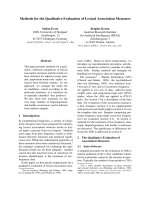
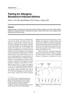
tions. Figure 1 shows reverse-cumulative distributions of the
number of tags per TSS for six human CAGE samples that
contain a total of a few million CAGE tags each. On the hori-
zontal axis is the number of tag t and on the vertical axis the
number of TSS positions to which at least t tags map. As the
figure shows, the distributions of tags per TSS are power-laws
to a very good approximation, spanning four orders of magni-
tude, and the slopes of the power-laws are a very similar
across samples. These samples are all from THP-1 cells both
untreated and after 24 hours of phorbol myristate acetate
(PMA) treatment. Very similar distributions are observed for
essentially all CAGE samples currently available (data not
shown).
The large majority of observed TSSs have only a very small
number of tags. These TSSs are often observed in only a single
sample, and seem to correspond to very low expression 'back-
ground transcription'. On the other end of the scale there are
TSSs that have as many as 10
4
tags, that is, close to 1% of all
tags in the sample. Manual inspection confirms that these
correspond to TSSs of genes that are likely to be highly
expressed, for example, cytoskeletal or ribosomal proteins. It
is quite remarkable in the opinion of these authors that both
low expression background transcription, whose occurrence

is presumably mostly stochastic, and the expression of the
highest expressed TSSs, which is presumably highly regu-
lated, occur at the extremes of a common underlying distribu-
tion. That this power-law expression distribution is not an
artifact of the measurement technology is suggested by the
fact that previous data from high-throughput serial analysis
of gene expression (SAGE) studies have also found power-law
distributions [14]. For ChIP-seq experiments, the number of
tags observed per region also appears to follow an approxi-
mate power-law distribution [15]. In addition, our analysis of
RNA-seq datasets from Drosophila shows that the number of
reads per position follows an approximate power-law distri-
bution as well (Figure S1 in Additional data file 1). These
observations strongly suggest that RNA expression data gen-
erally obey power-law distributions. The normalization pro-
cedure that we present here should thus generally apply to
deep sequencing expression data.
For each sample, we fitted (see Materials and methods) the
reverse-cumulative distribution of tags per TSS to a power-
law of the form:
with n
0
the inferred number of positions with at least t = 1 tag
and

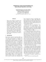
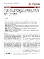
the slope of the power-law. Figure 2 shows the fitted
values of n
0
and


for all 56 human CAGE samples.
We see that, as expected, the inferred number of positions n
0
varies significantly with the depth of sequencing; that is, the
dots on the right are from the more recent samples that were
sequenced in greater depth. In contrast, the fitted exponents
vary relatively little around an average of approximately -
1.25, especially for the samples with large numbers of tags.
In the analysis of micro-array data it has become accepted
that it is beneficial to use so-called quantile normalization, in
which the expression values from different samples are trans-
formed to match a common reference distribution [16]. We
follow a similar approach here. We make the assumption that
the 'true' distribution of expression per TSS is really the same
in all samples, and that the small differences in the observed
reverse-cumulative distributions are the results of experi-
mental biases that are varying across samples. This includes
nt n t()= ,
0
−

(1)
Reverse cumulative distributions for the number of different TSS positions that have at least a given number of tags mapping to themFigure 1
Reverse cumulative distributions for the number of different TSS positions
that have at least a given number of tags mapping to them. Both axes are
shown on a logarithmic scale. The three red curves correspond to the
distributions of the three THP-1 cell control samples and the three blue
curves to the three THP-1 samples after 24 hours of phorbol myristate
acetate treatment. All other samples show very similar distributions (data
not shown).

1 10 100 1000 10000
Tag count t
1
10
100
1000
10000
100000
Num TSS ≥ t
Fitted off-sets n
0
(horizontal axis) and fitted exponents

(vertical axis) for the 56 human CAGE samples that have at least 100,000 tagsFigure 2
Fitted off-sets n
0
(horizontal axis) and fitted exponents

(vertical axis) for
the 56 human CAGE samples that have at least 100,000 tags.
0 50000 100000 150000 200000 250000 300000
Offset (num pos)
- 1.45
- 1.4
- 1.35
- 1.3
- 1.25
- 1.2
- 1.15
Exponent

Human
Genome Biology 2009, Volume 10, Issue 7, Article R79 Balwierz et al. R79.4
Genome Biology 2009, 10:R79
fluctuations in the fraction of tags that maps successfully, var-
iations in sequence-specific linker efficiency, the noise in PCR
amplification, and so on. To normalize our tag count, we map
all tags to a reference distribution. We chose as reference dis-
tribution a power-law with an exponent of

= -1.25 and, for
convenience, we chose the offset n
0
such that the total
number of tags is precisely 1 million. We then used the fits for
all samples to transform the tag-counts into normalized 'tags
per million' (TPM) counts (see Materials and methods). Fig-
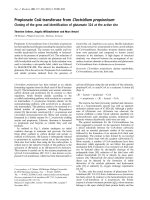
ure 3 shows the same six distributions as in Figure 1, but now
after the normalization.
Although the changes that this normalization introduces are
generally modest, the collapse of the distributions shown in
Figure 3 strongly suggests that the normalization improves
quantitative comparability of the expression profiles. Indeed,
as described below, for a replicate data-set in which two deep-
CAGE libraries were constructed from a common mRNA
sample, the normalization significantly reduces the apparent
variation between the replicates' expression profiles. Finally,
we note that normalization to a common power-law distribu-
tion has also been proposed for normalizing micro-arrays
[17].
In the remainder we will use the normalized tag counts to

compare the expression at individual positions in the genome
across samples. We also retain the raw tag-counts because, as
we will see below, the noise on the observed tag count
depends on these raw counts.
Noise model
In order to analyze expression profiles, it is necessary to ana-
lyze the distribution of the noise on deepCAGE and other
deep-sequencing expression measurements. To our knowl-
edge, such an analysis has not yet been performed. Instead of
determining noise on expression measurements, existing
work has focused on defining models of the background dis-
tribution of tags/reads, which can be used to identify regions
that have significantly more mapped tags/reads than
expected from the background model. These background
models assume that the number of tags in a given region fol-
lows either a simple Poisson distribution, or a Poisson distri-
bution with gamma-distributed rate [18].
To quantitatively investigate the noise in the expression
measurements, we compared tag-counts across replicate
data-sets. Among the currently available CAGE data-sets
there is one pair in which two libraries were prepared from a
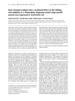
common mRNA sample and Figure 4 shows a scatter plot of
the normalized tag counts (TPM) from the replicate measure-
ments.
The figure shows that, at high TPM (that is, for positions with
TPMs larger than e
4
 55), the scatter has an approximately
constant width whereas at low TPM the width of the scatter
increases dramatically. This kind of funnel shape is familiar

from micro-array expression data where the increase in noise
at low expression is caused by the contribution of non-specific
background hybridization. However, for the deepCAGE data
this noise is of an entirely different origin.
In deep sequencing experiments the noise comes from essen-
tially two separate processes. First, there is the noise that is
introduced in going from the biological input sample to the
final library that goes into the sequencer. Second, there is the
noise introduced by the sequencing itself. For the CAGE
experiments the former includes cap-trapping, linker liga-
tion, cutting by the restriction enzyme, PCR amplification,
Normalized reverse cumulative distributions for the number of different TSS positions that have at least a given number of tags mapping to themFigure 3
Normalized reverse cumulative distributions for the number of different
TSS positions that have at least a given number of tags mapping to them.
Both axes are shown on a logarithmic scale. The three red curves
correspond to the distributions of the three THP-1 control samples and
the three blue curves to the three THP-1 samples after 24 hours of PMA
treatment.
1 10 100 1000 10000
Tag count t
1
10
100
1000
10000
100000.
Num TSS ≥ t
CAGE replicate from THP-1 cells after 8 hours of lipopolysaccharide treatmentFigure 4
CAGE replicate from THP-1 cells after 8 hours of lipopolysaccharide
treatment. For each position with mapped tags, the logarithm of the

number of tags per million (TPM) in the first replicate is shown on the
horizontal axis, and the logarithm of the number of TPM in the second
replicate on the vertical axis. Logarithms are natural logarithms.
0 2 4 6 8 10
0
2
4
6
8
10
Log[tpm] replicate 1
Log[tpm] replicate 2
Genome Biology 2009, Volume 10, Issue 7, Article R79 Balwierz et al. R79.5
Genome Biology 2009, 10:R79
and concatenation of the tags. In other deep-sequencing
experiments, for example, RNA-seq or ChIP-seq with Solexa
sequencing, there will similarly be processes such as the
shearing or sonication of the DNA, adding of the linkers, and
growing clusters on the surface of the flow cell.
With respect to the noise introduced by the sequencing itself,
it seems reasonable to assume that the N tags that are eventu-
ally sequenced can be considered a random sample of size N
of the material that went into the sequencer. This will lead to
relatively large 'sampling' noise for tags that form only a small
fraction of the pool. For example, assume that a particular tag
has fraction f in the tag pool that went into the sequencer.
This tag is expected to be sequenced Όn΍ = fN times among the
N sequenced tags, and the actual number of times n that it is
sequenced will be Poisson distributed according to:
Indeed, recent work [19] shows that the noise in Solexa

sequencing itself (that is, comparing different lanes of the
same run) is Poisson distributed. It is clear, however, that the
Poisson sampling is not the only source of noise. In Figure 4
there is an approximately fixed width of the scatter even at
very high tag-counts, where the sampling noise would cause
almost no difference in log-TPM between replicates. We thus
conclude that, besides the Poisson sampling, there is an addi-
tional noise in the log-TPM whose size is approximately inde-
pendent of the total log-TPM. Note that noise of a fixed size
on the log-TPM corresponds to multiplicative noise on the
level of the number of tags. It is most plausible that this mul-
tiplicative noise is introduced by the processes that take the
original biological samples into the final samples that are
sequenced; for example, linker ligation and PCR amplifica-
tion may vary from tag to tag and from sample to sample. The
simplest, least biased noise distribution, assuming only a
fixed size of the noise, is a Gaussian distribution [20].
We thus model the noise as a convolution of multiplicative
noise, specifically a Gaussian distribution of log-TPM with
variance

2
, and Poisson sampling. As shown in the methods,
if f is the original frequency of the TSS in the mRNA pool, and
a total of N tags are sequenced, then the probability to obtain
the TSS n times is approximately:
where the variance

2
(n) is given by:

That is, the measured log-TPM is a Gaussian whose mean
matches the log-TPM in the input sample, with a variance
equal to the variance of the multiplicative noise (

2
) plus one
over the raw number of measured tags. The approximation
(Equation 3) breaks down for n = 0. The probability to obtain
n = 0 tags is approximately given by (Materials and methods):
We used the CAGE technical replicate (Figure 4) to estimate
the variance

2
of the multiplicative noise (Materials and
methods) and find

2
= 0.085. To illustrate the impact of the
normalization, determining

2
on the same unnormalized
data-set, we obtained

2
= 0.11, that is, a 29% increase in the
apparent noise between the replicates. In addition to this rep-
licate, among the human CAGE data-sets there is a time
course of THP-1 cells after PMA treatment, measured in trip-
licate, which includes samples before PMA treatment and

after only 1 hour of PMA treatment. Manual inspection shows
that the correlation of tags per TSS for these two samples is as
large as for the technical replicate. This makes sense because,
on the time scale of 1 hour, the expression of most transcripts
can probably not change appreciably [21]. Using a procedure
(Materials and methods) that takes into account that a small
fraction of TSSs may change expression significantly between
the two samples, we estimated

2
as well for the three 0/1
hour sample pairs. The values we estimate are, respectively,

2
= 0.048,

2
= 0.116, and

2
= 0.058.
In summary, using four pairs of samples that are (almost)
replicates, we find estimates of

2
ranging from 0.048 to
0.116. Although this analysis provides some evidence that the
size of the multiplicative noise varies between samples, the
range of inferred values is small and we will make the
assumption that


2
is the same for all samples. As an estimate
of

2
we took an intermediate value of

2
= 0.06 for the rest of
our CAGE analysis.
We next validated this noise model as follows. According to
our noise model, for TSSs that have non-zero expression in
both samples, the z-statistic:
with m' the normalized expression at 1 hour and n' at zero
hours, should be Gaussian distributed with standard devia-
tion 1 (Materials and methods). We tested this for the three
biological replicates at 0/1 hour and for the technical repli-
cate. Figure 5 shows this theoretical distribution (in black)
together with the observed histogram of z-values for the four
replicates.
Although the data are noisy, it is clear that all three curves
obey a roughly Gaussian distribution. Note the deviation
Pn f N
fN
n
n
e
Nf
(|, )=

!
.
()
−
(2)
Pn f N
nN f
n
nn
(|,, )=
((/) ())
2
2()
2
2()
,



exp
log log
−
−
⎛
⎝
⎜
⎜
⎞
⎠
⎟

⎟
(3)

22
()=
1
.n
n
+
(4)
PfNe
fN
(0 | , , ) = .

−
(5)
z
nm
nm
=
() ( )
2
2
11
,
log log
′
−
′
++


(6)
Genome Biology 2009, Volume 10, Issue 7, Article R79 Balwierz et al. R79.6
Genome Biology 2009, 10:R79
from the theoretical curve at very low z, that is, z < -4, which
appears only for the 0/1 hour comparisons. These correspond
to the small fraction of positions that are significantly up-reg-
ulated at 1 hour. In summary, Figure 5 clearly shows that the
data from the replicate experiments are well described by our
noise model.
To verify the applicability of our noise model to RNA-seq
data, we used two replicate data sets of Drosophila mRNA
samples that were sequenced using Solexa sequencing and
estimated a value of

2
= 0.073 for these replicate samples
(Figure S2 in Additional data file 1). This fitted value of

2
is
similar to those obtained for the CAGE samples.
Finally, the

2
values that we infer for the deep sequencing
data are somewhat larger than what one typically finds for
replicate expression profiles as measured by micro-arrays.
However, it is important to stress that CAGE measures
expression of individual TSSs, that is, single positions on the

genome, whereas micro-arrays measure the expression of an
entire gene, typically by combining measurements from mul-
tiple probes along the gene. Therefore, the size of the 'noise'
in CAGE and micro-array expression measurements cannot
be directly compared. For example, when CAGE measure-
ments from multiple TSSs associated with the same gene are
combined, expression profiles become significantly less noisy
between replicates (

2
= 0.068 versus

2
= 0.085; Figures S4
and S5 in Additional data file 1). This applies also to RNA-seq
data (

2
= 0.02 versus

2
= 0.073; Figure S2 and S3 in Addi-
tional data file 1).
Promoterome construction
Using the methods outlined above on CAGE data, we can
comprehensively identify TSSs genome-wide, normalize their
expression, and quantitatively characterize the noise distri-
bution in their expression measurements. This provides the
most detailed information on transcription starts and, from
the point of view of characterizing the transcriptome, there is,

in principle, no reason to introduce additional analysis.
However, depending on the problem of interest, it may be
useful to introduce additional filtering and/or clustering of
the TSSs. For example, whereas traditionally it has been
assumed that each 'gene' has a unique promoter and TSS,
large-scale sequence analyses, such as performed in the
FANTOM3 project [8], have made it clear that most genes are
transcribed in different isoforms that use different TSSs.
Alternative TSSs not only involve initiation from different
areas in the gene locus - for example, from different starting
exons - but TSSs typically come in local clusters spanning
regions ranging from a few to over 100 bp wide.
These observations raise the question as to what an appropri-
ate definition of a 'basal promoter' is. Should we think of each
individual TSS as being driven by an individual 'promoter',
even for TSSs only a few base-pairs apart on the genome? The
answer to this question is a matter of definition and the
appropriate choice depends on the application in question.
For example, for the FANTOM3 study the main focus was to
characterize all distinct regions containing a significant
amount of transcription initiation. To this end the authors
simply clustered CAGE tags whose genomic mappings over-
lapped by at least 1 bp [8]. Since CAGE tags are 20 to 21 bp
long, this procedure corresponds to single-linkage clustering
of TSSs within 20 to 21 bp of each other. A more recent pub-
lication [22] creates a hierarchical set of promoters by identi-
fying all regions in which the density of CAGE tags is over a
given cut-off. This procedure thus allows one to identify all
distinct regions with a given total amount of expression for
different expression levels and this is clearly an improvement

over the ad hoc clustering method employed in the
FANTOM3 analysis.
Both clustering methods just mentioned cluster CAGE tags
based only on the overall density of mapped tags along the
genome - that is, they ignore the expression profiles of the
TSSs across the different samples. However, a key question
that one often aims to address with transcriptome data is how
gene expression is regulated. That is, whereas these methods
can successfully identify the distinct regions from which tran-
scription initiation is observed, they cannot detect whether
the TSSs within a local cluster are similarly expressed across
samples or that different TSSs in the cluster have different
expression profiles. Manual inspection shows that, whereas
there are often several nearby TSSs with essentially identical
expression profiles across samples/tissues, one also finds
cases in which TSSs that are only a few base-pairs apart show
clearly distinct expression profiles. We hypothesize that, in
the case of nearby co-expressed TSSs, the regulatory mecha-
nisms recruit the RNA polymerase to the particular area on
the DNA but that the final TSS that is used is determined by
an essentially stochastic (thermodynamic) process. One
could, for example, imagine that the polymerase locally slides
Observed histograms of z-statistics for the three 0/1 hour (in red, dark blue, and light blue) samples and for the technical replicate (in yellow) compared with the standard unit Gaussian (in black)Figure 5
Observed histograms of z-statistics for the three 0/1 hour (in red, dark
blue, and light blue) samples and for the technical replicate (in yellow)
compared with the standard unit Gaussian (in black). The vertical axis is
shown on a logarithmic scale.
-4 -2 0 2 4
z
0.00001

0.0001
0.001
0.01
0.1
1
Frequency
Genome Biology 2009, Volume 10, Issue 7, Article R79 Balwierz et al. R79.7
Genome Biology 2009, 10:R79
back and forth on the DNA and chooses a TSS based on the
affinity of the polymerase for the local sequence, such that dif-
ferent TSSs in the area are used in fixed relative proportions.
In contrast, when nearby TSSs show different expression pro-
files one could imagine that there are particular regulatory
sites that control initiation at individual TSSs.
Whatever the detailed regulatory mechanisms are, it is clear
that, for the study of transcription regulation, it is important
to properly separate local clusters of TSSs that are co-regu-
lated from those that show distinct expression profiles. Below
we present a Bayesian methodology that clusters nearby TSSs
into 'transcription start clusters' (TSCs) that are co-expressed
in the sense that their expression profiles are statistically
indistinguishable.
A second issue is that, as shown by the power-law distribution
of tags per TSS (Figure 1), we find a very large number of dif-
ferent TSSs used in each sample and the large majority of
these have very low expression. Many TSSs have only one or
a few tags and are often observed in one sample only. From
the point of view of studying the regulation of transcription, it
is clear that one cannot meaningfully speak of 'expression
profiles' of TSSs that were observed only once or twice and

only in one sample. That is, there appears to be a large
amount of 'background transcription' and it is useful to sepa-
rate these TSSs that are used very rarely, and presumably
largely stochastically, from TSSs that are significantly
expressed in at least one sample. Below we also provide a sim-
ple method for filtering such 'background transcription'.
Finally, for each significantly expressed TSC there will be a
'proximal promoter region' that contains regulatory sites that
control the rate of transcription initiation from the TSSs
within the TSC. Since TSCs can occur close to each other on
the genome, individual regulatory sites may sometimes be
controlling multiple nearby TSCs. Therefore, in addition to
clustering nearby TSSs that are co-expressed, we introduce an
additional clustering layer, in which TSCs with overlapping
proximal promoters are clustered into 'transcription start
regions' (TSRs). Thus, whereas different TSSs may share reg-
ulatory sites, the regulatory sites around a TSR only control
the TSSs within the TSR.
Using the normalization method and noise model described
above, we have constructed comprehensive 'promoteromes'
of the human and mouse genomes from 122 CAGE samples
across different human and mouse tissues and conditions
(Materials and methods) by first clustering nearby co-regu-
lated TSSs; second, filtering out background transcription;
third, extracting proximal promoter regions around each TSS
cluster; and fourth merging TSS clusters with overlapping
proximal promoters into TSRs. We now describe each of these
steps in the promoterome construction.
Clustering adjacent co-regulated transcription start sites
We define TSCs as sets of contiguous TSSs on the genome,

such that each TSS is relatively close to the next TSS in the
cluster, and the expression profiles of all TSSs in the cluster
are indistinguishable up to measurement noise. To construct
TSCs fitting this definition, we will use a Bayesian hierarchi-
cal clustering procedure that has the following ingredients.
We start by letting each TSS form a separate, 1-bp wide TSC.
For each pair of neighboring TSCs there is prior probability

(d) that these TSCs should be fused, which depends on the
distance d along the genome between the two TSCs. For each
pair of TSCs we calculate the likelihoods of two models for the
expression profiles of the two TSCs. The first model assumes
that the two TSCs have a constant relative expression in all
samples (up to noise). The second model assumes that the
two expression profiles are independent. Combining the prior

(d) and likelihoods of the two models, we calculate, for each
contiguous pair of TSCs, a posterior probability that the two
TSCs should be fused. We identify the pair with highest pos-
terior probability and if this posterior probability is at least 1/
2, we fuse this pair and continue clustering the remaining
TSCs. Otherwise the clustering stops.
The details of the clustering procedure are described in Mate-
rials and methods. Here we will briefly outline the key ingre-
dients. The key quantity for the clustering is the likelihood
ratio of the expression profiles of two neighboring TSCs under
the assumptions that their expression profiles are the same
and independent, respectively. That is, if we denote by x
s
the

logarithm of the TPM in sample s of one TSC, and by y
s
the
log-TPM in sample s of a neighboring TSC, then we want to
calculate the probability P({x
s
}, {y
s
}) of the two expression
profiles assuming the two TSCs are expressed in the same
way, and the probability P({x
s
}), P({y
s
}) of the two expression
profiles assuming they are independent.
For a single TSS we write x
s
as the sum of a mean expression

, the sample-dependent deviation

s
from this mean, and a
noise term:
The probability P(x
s
|

+


s
) is given by the noise-distribution
(Equation 3). To calculate the probability P({x
s
}) of the
expression profile, we assume that the prior probability P(

)
of

is uniformly distributed and that the prior probabilities of
the

s
are drawn from a Gaussian with variance

, that is:
The probability of the expression profile of a single TSC is
then given by integrating out the unknown 'nuisance' varia-
bles {

s
} and

:
x
ss
=.noise ++


(7)
P
ss
(|)=
22
() .
2





exp −
⎡
⎣
⎢
⎤
⎦
⎥
(8)
Genome Biology 2009, Volume 10, Issue 7, Article R79 Balwierz et al. R79.8
Genome Biology 2009, 10:R79
The parameter

, which quantifies the a priori expected
amount of expression variance across samples, is determined
by maximizing the joint likelihood of all TSS expression pro-
files (Materials and methods).
To calculate the probability P({x
s

}, {y
s
}), we assume that even
though the two TSCs may have different mean expressions,
their deviations

s
are the same across all samples. That is, we
write:
and
The probability P({x
s
}, {y
s
}) is then given by integrating out
the nuisance parameters:
As shown in the Materials and methods section, the integrals
in Equations 9 and 12 can be done analytically. For each
neighboring pair of TSCs we can thus analytically determine
the log-ratio:
To perform the clustering, we also need a prior probability
that two neighboring TSCs should be fused and we will
assume that this prior probability depends only on the dis-
tance between the two TSCs along the genome. That is, for
closely spaced TSC pairs we assume it is a priori more likely
that they are driven by a common promoter than for distant
pairs of TSCs. To test this, we calculated the log-ratio L of
Equation 13 for each consecutive pair of TSSs in the human
CAGE data. Figure 6 shows the average of L as a function of
the distance of the neighboring TSSs.

Figure 6 shows that the closer the TSSs, the more likely they
are to be co-expressed. Once TSSs are more than 20 bp or so
apart, they are not more likely to be co-expressed than TSSs
that are very far apart. To reflect these observations, we will
assume that the prior probability

(d) that two neighboring
TSCs are co-expressed falls exponentially with their distance
d, that is:
where l is a length-scale that we set to l = 10.
For each consecutive pair of TSCs we calculate L and we cal-
culate a prior log-ratio:
where the distance d between two TSCs is defined as the dis-
tance between the most highly expressed TSSs in the two
TSCs. We iteratively fuse the pair of TSCs for which L + R is
largest. After each fusion we of course need to update R and L
for the neighbors of the fused pair. We keep fusing pairs until
there is no longer any pair for which L + R > 0 (corresponding
to a posterior probability of 0.5 for the fusion).
Filtering background transcription
If one were principally interested in identifying all transcrip-
tion initiation sites in the genome, one would of course not fil-
ter the set of TSCs obtained using the clustering procedure
just described. However, when one is interested in studying
regulation of expression then one would want to consider
only those TSCs that show a substantial amount of expression
in at least one sample and remove 'background transcription'.
To this end we have to determine a cut-off on expression level
to separate background from significantly expressed TSCs. As
the distribution of expression per TSS does not naturally sep-

arate into a high expressed and low expressed part - that is, it
is power-law distributed - this filtering is, to some extent,
arbitrary.
According to current estimates, there are a few hundred thou-
sand mRNAs per cell in mammals. In our analysis we have
made the choice to retain all TSCs such that, in at least one
sample, at least ten TPM derive from this TSC, that is, at least
1 in 100,000 transcripts. With this conservative cut-off we
Px dP dPx P
s
s
ss s s
({ }) = ( ) ( | ) ( | ) .
∫
∏
∫
+
⎡
⎣
⎢
⎤
⎦
⎥
   
(9)
x
ss
=,noise ++

(10)

y
ss
=noise++


(11)
Px y ddP P d Px Py P
ss
s
ss s s s
({ },{ })= ()() ( | )( | )(
∫
∏
∫
++
        
 
ss
|).

⎡
⎣
⎢
⎤
⎦
⎥
(12)
L
Px
s

y
s
Px
s
Py
s
=
({ },{ })
({ }) ({ })
.log
⎡
⎣
⎢
⎤
⎦
⎥
(13)

()= ,
/
de
dl−
(14)
R
d
d
=
()
1()
,log



−
⎛
⎝
⎜
⎞
⎠
⎟
(15)
Average log-ratio L (Equation 13) for neighboring pairs of individual TSSs as a function of the distance between the TSSsFigure 6
Average log-ratio L (Equation 13) for neighboring pairs of individual TSSs
as a function of the distance between the TSSs. The horizontal axis is
shown on a logarithmic scale.
1 2 5 10 20 50 100 200 500 1000
Distance TSS pair
0.1
0.2
0.3
0.4
0.5
Average log- likelihood ratio
1 2 5 10 20 50 100 200 500 1000
Genome Biology 2009, Volume 10, Issue 7, Article R79 Balwierz et al. R79.9
Genome Biology 2009, 10:R79
ensure that there is at least one mRNA per cell in at least one
sample. Since for some samples the total number of tags is
close to 100,000, a TSC may spuriously pass this threshold by
having only 2 tags in a sample with low total tag count. To
avoid these, we also demand that the TSC has one tag in at

least two different samples.
Proximal promoter extraction and transcription start region
construction
Finally, for each of the TSCs we want to extract a proximal
promoter region that contains regulatory sites that control
the expression of the TSC, and, in addition, we want to cluster
TSCs with overlapping proximal promoter regions. To esti-
mate the typical size of the proximal promoters, we investi-
gated conservation statistics in the immediate neighborhood
of TSCs. For each human TSC we extracted PhastCons [23]
scores 2.5 kb upstream and downstream of the highest
expressed TSS in the TSC and calculated average PhastCons
scores as a function of position relative to TSS (Figure 7).
We observe a sharp peak in conservation around the TSS,
suggesting that the functional regulatory sites are highly con-
centrated immediately around it. Upstream of the TSS the
conservation signal decays within a few hundred base-pairs,
whereas downstream of the TSS the conservation first drops
sharply and then more slowly. The longer tail of conservation
downstream of the TSS is most likely due to selection on the
transcript rather than on transcription regulatory sites.
Based on these conservation statistics, we conservatively
chose the region from -300 to +100 with respect to the TSS as
the proximal promoter region. Although the precise bounda-
ries are, to some extent, arbitrary, it is clear that the con-
served region peaks in a narrow region of only a few hundred
base-pairs wide around the TSS. As a final step in the con-
struction of the promoteromes, we clustered together all TSCs
whose proximal promoter regions (that is, from 300 bp
upstream of the first TSS in the TSC to 100 bp downstream of

the last TSS in the TSC) overlap into TSRs.
Promoterome statistics
To characterize the promoteromes that we obtained, we com-
pared them with known annotations and we determined a
number of key statistics.
Comparison with starts of known transcripts
Using the collection of all human mRNAs from the UCSC
database [24], we compared the location of our TSCs with
known mRNA starts. For each TSC we identified the position
of the nearest known TSS; Figure 8 shows the distribution of
the number of TSCs as a function of the relative position of the
nearest known mRNA start.
By far the most common situation is that there is a known
mRNA start within a few base-pairs of the TSC. We also
observe a reasonable fraction of cases where a known mRNA
start is somewhere between 10 and 100 bp either upstream or
downstream of the TSC. Known TSSs more than 100 bp from
a TSC are relatively rare and the frequency drops further with
distance, with only a few cases of known mRNA starts 1,000
bp away from a TSC. For 37.7% of all TSCs there is no known
mRNA start within 1,000 bp of the TSC, and for 27% there is
no known mRNA start within 5 kb. We consider these latter
27% of TSCs novel TSCs. To verify that the observed conser-
vation around TSSs shown in Figure 7 is not restricted to TSSs
near known mRNA starts, we also constructed a profile of
average PhastCons scores around these novel TSCs (Figure
9).
Average PhastCons (conservation) score relative to TSSs of genomic regions upstream and downstream of all human TSCsFigure 7
Average PhastCons (conservation) score relative to TSSs of genomic
regions upstream and downstream of all human TSCs. The vertical lines

show positions -300 and +100 with respect to TSSs.
- 2000 - 1000 0 1000 2000
Position relative to TSS
0.1
0.15
0.2
0.25
0.3
Average PhastCons score
The number of TSCs as a function of their position relative to the nearest known mRNA startFigure 8
The number of TSCs as a function of their position relative to the nearest
known mRNA start. Negative numbers mean the nearest known mRNA
start is upstream of the TSC. The vertical axis is shown on a logarithmic
scale. The figure shows only the 46,293 TSCs (62.3%) that have a known
mRNA start within 1,000 bp.
- 1000 - 500 0 500 1000
10
100
1000
10
4
Position of closest known start
Number of TSCs
Distances Human TSCs to known transcripts
Genome Biology 2009, Volume 10, Issue 7, Article R79 Balwierz et al. R79.10
Genome Biology 2009, 10:R79
We observe a similar peak to that for all TSCs, although its
height is a bit lower and the peak appears a bit more symmet-
rical, showing only marginally more conservation down-
stream than upstream of TSSs. Although we can only

speculate, one possible explanation for the more symmetrical
conservation profile of novel TSCs is that this class of TSCs
might contain transcriptional enhancers that show some
transcription activity themselves. In Additional data file 1 we
present analogous figures for the mouse promoterome.
Hierarchical structure of the promoterome
Table 1 shows the total numbers of CAGE tags, TSCs, TSRs,
and TSSs within TSCs that we found for the human and
mouse CAGE data-sets.
The 56 human CAGE samples identify about 74,000 TSCs
and the 66 mouse samples identify about 77,000 TSCs.
Within these TSCs there are about 861,000 and 608,000
individual TSSs, respectively, corresponding to about 12 TSSs
per TSC in human and about 8 TSSs per TSC in mouse. Note
that, while large, this number of TSSs is still much lower than
the total numbers of unique TSSs that were observed. This
again underscores the fact that the large majority of TSSs are
expressed at very low levels.
Next we investigated the hierarchical structure of the human
promoterome (similar results were obtained in mouse (see
Additional data file 1). Figure 10 shows the distributions of
the number of TSSs per TSC, the number of TSSs per TSR,
and the number of TSCs per TSR.
Figure 10b shows that the number of TSCs per TSR is essen-
tially exponentially distributed. That is, it is most common to
find only a single TSC per TSR, TSRs with a handful of TSCs
are not uncommon, and TSRs with more than ten TSCs are
very rare. The number of TSSs per TSC is more widely distrib-
uted (Figure 10a). It is most common to find one or two TSSs
in a TSC, and the distribution drops quickly with TSS number.

However, there is a significant tail of TSCs with between 10
and 50 or so TSSs. The observation that the distribution of the
number of TSSs per TSC has two regimes is even clearer from
Figure 10c, which shows the distribution of the number of
TSSs per TSR. Here again we see that it is most common to
find one or two TSSs per TSR, and that TSRs with between
five and ten TSSs are relatively rare. There is, however, a fairly
wide shoulder in the distribution corresponding to TSRs that
have between 10 and 50 TSSs. These distributions suggest
that there are two types of promoters: 'specific' promoters
with at most a handful of TSSs in them, and more 'fuzzy' pro-
moters with more than ten TSSs.
This observation is further supported by the distribution of
the lengths of TSCs and TSRs (Figure 11). In particular, the
distribution of the length of TSRs (Figure 11b) also shows a
clear shoulder involving lengths between 25 and 250 bp or so.
Comparison with simple single-linkage clustering
In Additional data file 1 we compare the promoteromes
obtained with our clustering procedure with those that were
obtained with the simple single-linkage clustering procedures
used in FANTOM3. The key difference between our clustering
and the single-linkage clustering employed in FANTOM3 is
that, in our procedure, neighboring TSSs with significantly
different expression profiles are not clustered. Although TSSs
within a few base-pairs of each other on the genome often
show correlated expression profiles, it is also quite common
to find nearby TSSs with significantly differing expression
profiles. Figure 12 shows two examples of regions that contain
multiple TSSs close to each other on the genome, where some
TSSs clearly correlate in expression whereas others do not.

Within a region less than 90 bp wide our clustering identifies
5 different TSCs that each (except for the furthest down-
stream TSC) contain multiple TSSs with similar expression
profiles. Any clustering algorithm that ignores expression
profiles across samples would likely cluster all these TSSs into
Average PhastCons (conservation) score relative to TSSs of genomic regions upstream and downstream of 'novel' human TSCs that are more than 5 kb away from the start of any known transcriptFigure 9
Average PhastCons (conservation) score relative to TSSs of genomic
regions upstream and downstream of 'novel' human TSCs that are more
than 5 kb away from the start of any known transcript.
- 2000 - 1000 0 1000 2000
0.10
0.15
0.20
0.25
0.30
Position relative to TSS
Average PhastCons score
Table 1
Global statistics of the human and mouse 'promoteromes' that
we constructed from the human and mouse CAGE data
Statistic Human Mouse
Number of samples 56 66
Number of mapped CAGE tags 25,469,648 8,104,796
Number of TSSs 6,395,686 1,515,273
Number of TSSs in TSCs 860,823 608,474
Number of TSCs 74,273 77,286
Number of TSRs 43,164 50,915
Shown are the number of different samples, the total number of CAGE
tags that were mapped to the genome, the total number of different
TSSs that were observed at least once, the number of TSSs in TSCs,

the number of TSCs, and the number of TSRs.
Genome Biology 2009, Volume 10, Issue 7, Article R79 Balwierz et al. R79.11
Genome Biology 2009, 10:R79
one large TSC. However, as shown in Figure 12c for the red
and blue colored TSCs, their expression profiles across sam-
ples are not correlated at all. A scatter plot of the expression
in TPM of the red and blue colored TSCs is shown in Figure
S8 in Additional data file 1, and an additional example analo-
gous to Figure 12 is also shown (Figure S9).
Since clustering procedures that ignore expression profiles,
such as the single-linkage clustering employed in FANTOM3,
cluster nearby TSSs with quite dissimilar expression profiles,
one would expect that this clustering would tend to 'average
out' expression differences across samples. To test this, we
calculated for each TSC the standard deviation in expression
(log-TPM) for both our TSCs and those obtained with the
FANTOM3 clustering. Figure 13 shows the reverse cumula-
tive distributions of the standard deviations for the two sets of
TSCs. The figure shows that there is a substantial decrease in
the expression variation of the TSCs obtained with the
FANTOM3 clustering compared to the TSCs obtained with
our clustering. This illustrates that, as expected, clustering
without regard for the expression profiles of neighboring
TSSs leads to averaging out of expression variations. As a con-
sequence, for TSCs obtained with our clustering procedure
one is able to detect significant variations in gene expression,
and, thus, potential important regulatory effects that are
undetectable when one uses a clustering procedure that
ignores expression profiles.
High and low CpG promoters

Our promoterome statistics above suggest that there are two
classes of promoters. That there are two types of promoters in
mammals was already suggested in previous CAGE analyses
[8], where the wide and fuzzy promoters were suggested to be
associated with CpG islands, whereas promoters with a
TATA-box tended to be narrow. To investigate this, we calcu-
lated the CG and CpG content of all human promoters. That
is, for each TSR we determined the fraction of all nucleotides
that are either C or G (CG content), and the fraction of all
dinucleotides that are CpG (CpG content). Figure 14 shows
Hierarchical structure of the human promoteromeFigure 10
Hierarchical structure of the human promoterome. (a) Distribution of the number of TSSs per co-expressed TSC. (b) Distribution of the number of
TSCs per TSR. (c) Distribution of the number of TSSs per TSR. The vertical axis is shown on a logarithmic scale in all panels. The horizontal axis is shown
on a logarithmic scale in (a, c).
1 5 10 50 100 500
1
10
100
1000
10000
Numberof TSSs
Numberof TSCs
Distributionof TSSsperTSC
10 20 30 40 50
1
10
100
1000
10000
Numberof TSCs

Numberof TSRs
Distributionof TSCsperTSR
1 5 10 50 100 500
1
10
100
1000
10000
Numberof TSSs
Numberof TSRs
Distributionof TSSsperTSR
(a)
(b) (c)
Length (base pairs along the genome) distribution of (a) TSCs and (b) TSRsFigure 11
Length (base pairs along the genome) distribution of (a) TSCs and (b) TSRs. Both axes are shown on logarithmic scales in both panels.
1 5 10 50 100 500 1000
Length
0.1
1
10
100
1000
10000
Number of TSCs
Distribution of lengths of TSCs
1 10 100 1000
Length
0.1
10
1000

Number of TSRs
Distribution of lengths of TSRs
(a)
(b)
Genome Biology 2009, Volume 10, Issue 7, Article R79 Balwierz et al. R79.12
Genome Biology 2009, 10:R79
the two-dimensional histogram of CG and CpG content of all
human TSRs.
Figure 14 clearly shows that there are two classes of TSRs with
respect to CG and CpG content. Although it has been demon-
strated previously that CpG content of promoters shows a
bimodal distribution [25], the simultaneous analysis of both
CG and CpG content allows for a more efficient separation of
the two classes, and demonstrates more clearly that there are
really only two classes of promoters. We devised a Bayesian
procedure to classify each TSR as high-CpG or low-CpG
(Materials and methods) that allows us to unambiguously
classify the promoters based on their CG and CpG content. In
particular, for more than 91% of the promoters the posterior
probability of the high-CpG class was either > 0.95 or < 0.05.
To study the association between promoter class and its
length distribution, we selected all TSRs that with posterior
probability 0.95 or higher belong to the high-CpG class, and
all TSRs that with probability 0.95 or higher belong to the low
CpG class, and separately calculated the length distributions
of the two classes of TSRs.
Figure 15 shows that the length distributions of high-CpG and
low-CpG TSRs are dramatically different, supporting obser-
vations made with previous CAGE data [8]. For example, for
the high-CpG TSRs only 22% have a width of 10 bp or less. In

contrast, for the low-CpG TSRs approximately 80% of the
TSRs have a width of 10 bp or less. In summary, our analysis
supports that there are two promoter classes in human: one
class associated with low CpG content, low CG content, and
narrow TSRs, and one class associated with high CpG con-
Nearby TSCs with significantly differing expression profilesFigure 12
Nearby TSCs with significantly differing expression profiles. (a) A 90-bp region on chromosome 3 containing 5 TSCs (colored segments) and the start of
the annotated locus of the SENP5 gene (black segment). (b) Positions of the individual TSSs in the TSC and their total expression, colored according to the
TSC to which each TSS belongs. (c) Expression across the 56 CAGE samples for the red and blue colored TSCs.
TSC_hg18_v1_chr3_+_198079187
TSC_hg18_v1_chr3_+_198079167
TSC_hg18_v1_chr3_+_198079151
SENP5: SUMO1/sentrin specific peptidase 5
TSC_hg18_v1_chr3_+_198079198
TSC_hg18_v1_chr3_+_198079205
(a)
(b)
(c)
Chromosome 3 position
198079120
198079130
198079140
198079150
198079160
198079170
198079180
198079190
198079200
198079210
1

10
100
1000
TSS expr ession [tpm]
TSC_hg18_v1_chr3_+_198079151
TSC_hg18_v1_chr3_+_198079167
TSC_hg18_v1_chr3_+_198079187
TSC_hg18_v1_chr3_+_198079198
TSC_hg18_v1_chr3_+_198079205
Samples
10
100
TSC expr ession [tpm]
TSC_hg18_v1_chr3_+_198079167
TSC_hg18_v1_chr3_+_198079187
Reverse cumulative distributions of the standard deviation in expression across the 56 CAGE samples for the TSCs obtained with our clustering procedure (red) and the FANTOM3 single-linkage clustering procedure (green)Figure 13
Reverse cumulative distributions of the standard deviation in expression
across the 56 CAGE samples for the TSCs obtained with our clustering
procedure (red) and the FANTOM3 single-linkage clustering procedure
(green).
Genome Biology 2009, Volume 10, Issue 7, Article R79 Balwierz et al. R79.13
Genome Biology 2009, 10:R79
tent, high CG content, and wide promoters. Similar results
were obtained for mouse TSRs (data not shown).
Finally, we compared the promoter classification of known
and novel TSRs. Of the 43,164 TSRs, 37.7% are novel - that is,
there is no known transcript whose start is within 5 kb of the
TSR. For both known and novel TSRs the classification into
high-CpG and low-CpG is ambiguous for about 8% of the
TSRs. However, whereas for known TSRs 56% are associated

with the high-CpG class, for novel TSRs 76% are associated
with the low-CpG class. This is not surprising given that high-
CpG promoters tend to be higher and more widely expressed
than low-CpG promoters - that is, they are much less likely to
not have been observed previously.
Conclusions
It is widely accepted that gene expression is regulated to a
large extent by the rate of transcription initiation. Currently,
regulation of gene expression is studied mostly with oligonu-
cleotide micro-array chips. However, most genes initiate
transcription from multiple promoters, and while different
promoters may be regulated differently, the micro-array will
typically only measure the sum of the isoforms transcribed
from the different promoters. In order to study gene regula-
tion, it is, therefore, highly beneficial to monitor the expres-
sion from individual TSSs genome-wide and deepCAGE
technology now allows us to do precisely that. The related
RNA-seq technology similarly provides significant benefits
over micro-arrays. We therefore expect that, as the cost of
deep sequencing continues to come down, deep sequencing
technologies will gradually replace micro-arrays for gene
expression studies.
Application of deep sequencing technologies for quantifying
gene expression is still in its infancy and, not surprisingly,
there are a number of technical issues that complicate inter-
pretation of the data. For example, different platforms exhibit
different sequencing errors at different rates and, currently,
these inherent biases are only partially understood. Similarly,
it is also clear that the processing of the input samples to pre-
pare the final libraries that are sequenced introduces biases

that are currently poorly understood and it is likely that many
technical improvements will be made over the coming years
to reduce these biases.
Apart from the measurement technology as such, an impor-
tant factor in the quality of the final results is the way in which
the raw data are analyzed. The development of analysis meth-
ods for micro-array data is very illustrative in this respect.
Two-dimensional histogram (shown as a heatmap) of the CG base content (horizontal axis) and CpG dinucleotide content (vertical axis) of all human TSRsFigure 14
Two-dimensional histogram (shown as a heatmap) of the CG base content (horizontal axis) and CpG dinucleotide content (vertical axis) of all human
TSRs. Both axes are shown on logarithmic scales.
0.2 0.3 0.4 0.5 0.6 0.7 0.8 0.9
0.05
0.1
0.15
0.2
GC content of proximal promoters (log−scale)
CpG content of proximal promoters (log−scale with 0.05 pseudocount)
Heatmap of promoter density in GC and CpG content
Genome Biology 2009, Volume 10, Issue 7, Article R79 Balwierz et al. R79.14
Genome Biology 2009, 10:R79
Several years of in-depth study passed before a consensus
started to form in the community regarding the appropriate
normalization, background subtraction, correction for
sequence biases, and noise model. We expect that gene
expression analysis using deep sequencing data will undergo
similar development in the coming years. Here we have pre-
sented an initial set of procedures for analyzing deep
sequencing expression data, with specific application to deep-
CAGE data.
Our available data suggest that, across all tissues and condi-

tions, the expression distribution of individual TSSs is a uni-
versal power-law. Interestingly, this implies that there is no
natural expression scale that distinguishes the large number
of TSSs that are expressed at very low rates - so-called back-
ground transcription - from the highly regulated expression
of the TSSs of highly expressed genes. That is, background
transcription and the TSSs of the most highly expressed genes
are just the extrema of a scale-free distribution. As we have
shown, by assuming that a common universal power-law
applies to all samples, we can normalize the expression data
from different deep sequencing data-sets. The fact that
expression profiles from SAGE and from RNA-seq using the
Solexa platform also show power-law distributions strongly
suggests that this normalization scheme is applicable to deep
sequencing expression data in general. It should be noted that
although all observed distributions are power-laws, there is
no a priori reason that mammalian cells should have a com-
mon power-law expression distribution across all tissues and
conditions. It is conceivable that, as more extensive data
become available in the future, we may find significant differ-
ences between the expression distributions in different tis-
sues.
The noise in the expression measured across different deep-
CAGE samples can be accurately modeled by a convolution of
multiplicative noise and Poisson sampling and we derived a
practical analytical approximation to the resulting noise dis-
tribution. Using replicate data-sets, we inferred the size of the
multiplicative noise for different samples and found it to vary
in a small range. In addition, analysis of Solexa RNA-seq data
from Drosophila showed multiplicative noise of similar size.

However, we expect that it is a simplification to assume that
the size of the multiplicative noise is identical in all experi-
ments, and in the future we will want to apply a more refined
analysis that takes into account the differences in the size of
the multiplicative noise for different samples. To this end it
will be important to design experiments such that at least one
replicate is available to estimate the size of the multiplicative
noise associated with a given experimental procedure.
The noise model allows us to rigorously assess the statistical
significance of measured expression differences across differ-
ent samples. In particular, we developed a Bayesian proce-
dure that calculates the probability that two TSSs have
identical expression profiles. Interestingly, we found that
TSSs that are less than 10 bp apart on the genome are much
more likely to be co-expressed than more distal neighboring
TSSs. Using these results, we clustered sets of nearby co-
expressed TSSs into TSCs that we propose are each regulated
by a common 'promoter'. Of course, our ability to detect sig-
nificant expression differences is limited by the number of
available samples and we expect that, as the number of avail-
able deepCAGE samples increases, the number of TSCs will
increase as well.
Comparative genomic analysis shows a strong peak in
sequence conservation restricted to a few hundred base-pairs
around TSSs. This suggests that the proximal promoter asso-
ciated with each TSC extends a few hundred base-pairs
around the TSSs in the TSC. Besides clustering nearby co-
expressed TSSs into TSCs, we also clustered TSCs whose
proximal promoters overlap into TSRs. Comparing the
sequence composition and widths of TSRs, we find that there

are two classes of promoters in the human and mouse
genomes. The first class corresponds to TSRs that are narrow,
almost always less than 10 bp wide, and that have low CG con-
tent as well as low CpG content. The second class corresponds
to TSRs that are wide, that is, anywhere from 25 to 250 bp
wide, and that are associated with CpG islands, that is, having
both a high CG content as well as a high CpG content. It seems
plausible that different mechanisms may be involved in the
regulation of these two classes of promoters.
Materials and methods
CAGE and RNA-seq expression data
All the samples used in this study were provided by the
RIKEN Genomic Sciences Center as well as its successor, the
Omics Science Center, and come from the FANTOM3, the
Reverse cumulative distribution of the lengths (base-pairs along the genome) of TSRs for high-CpG (red curve) and low-CpG (green curve) promotersFigure 15
Reverse cumulative distribution of the lengths (base-pairs along the
genome) of TSRs for high-CpG (red curve) and low-CpG (green curve)
promoters. The horizontal axis is shown on a logarithmic scale.
0
0.2
0.4
0.6
0.8
1
1 10 100 1000
Frac TSRs > L
Length L
Reverse cumulative TSR length distribution
Genome Biology 2009, Volume 10, Issue 7, Article R79 Balwierz et al. R79.15
Genome Biology 2009, 10:R79

FANTOM4, and several smaller projects. Each human sample
has at least 100,000 mapped tags, and each mouse sample at
least 50,000. The lists of all 56 human and 66 mouse samples,
with tissue/cell line name, treatment and accession numbers
are included in Additional data files 2 and 3. Whenever
assigned, accession numbers of the DNA Data Bank of Japan
are listed. Raw CAGE data of the FANTOM4 project are avail-
able at [9].
The CAGE protocol that was used has been described in [26].
The 143 C6 mouse hippocampus and h93, i02, i03 human
THP-1 libraries were produced using a more recent protocol
adapted to the 454 Life Sciences sequencer (Roche) as
described in the Methods section of [27]. The lengths of the
CAGE tags were 20 to 21 bp in all cases.
For the RNA-seq data total RNA was isolated from Dro-
sophila Kc cells using Trizol reagent. Purification of mRNA
and the generation of the cDNA library were performed fol-
lowing the Illumina protocol for mRNA sequencing. Primary
sequencing data analysis was done following the Illumina
Genome Analyzer software pipeline. ELAND (part of the Illu-
mina suite) was used for the alignment of short reads to the
Drosophila genome (release 5).
Normalization by fitting to a reference distribution
For each CAGE sample we fit the reverse-cumulative distribu-
tion n(t) of the number of TSSs with at least t tags to a power-
law. To robustly fit these power-laws across different samples
with different total numbers of tags, we remove the data from
the first and last order of magnitude along the vertical axis
and apply simple linear regression to the remaining data. As
a result, for each sample s there will be a fitted exponent


(s)
and a fitted offset n
0
(s).
For a reference distribution of the form n
r
(r
0
t
-

) the total
number of tags is given by:
where

(x) is the Riemann-zeta function. That is, the total
number of tags is determined by both r
0
and

. For the refer-
ence distribution we chose

= 1.25 and =
10
6
. Setting

= 1.25 in Equation 16 and solving for r

0
we find:
To map tag-counts from different samples to this common
reference, we transform the tag-count t in each sample into a
tag-count t' according to:
such that the distribution n(t') for this sample will match the
reference distribution, that is, n(t') = n
r
(t'). If the observed
distribution has tag-count distribution:
then in terms of t' this becomes:
Demanding that n(t') = n
r
(t') gives:
This equation is satisfied when

/

= 1.25, that is:
Using this and solving for

we find:
Noise model
We model the noise as a convolution of multiplicative Gaus-
sian noise and Poisson sampling noise. Assume that tags from
a given TSS position correspond to a fraction f of the tags in
the input pool. Let x = log(f) and let y be the log-frequency of
the tag in the final prepared sample that will be sequenced,
that is, for CAGE after cap-trapping, linking, PCR-amplifica-
tion, and concatenation. We assume that all these steps intro-

duce a Gaussian noise with variance

2
so that the probability
P(y|x,

) is given by:
We assume that the only additional noise introduced by the
sequencing is simply Poisson sampling noise. That is, the
probability to obtain n tags for this position, given y and given
that we sequence N tags in total is given by:
Combining these two distributions, we find that the probabil-
ity to obtain n tags given that the log-frequency in the input
pool was x is given by:
Trtr
t
==(),
=1
00
∞
−
∑


(16)
Tnt
t
r
=()=10
6

∑
r
0
=217,623.
(17)
tt t→
′
=


(18)
nt n t()= ,
0
−

(19)
nt n
t
()= .
0
/
′
′
⎛
⎝
⎜
⎞
⎠
⎟
−



(20)
rt n
t
0
1.25
0
/
() = .
′
′
⎛
⎝
⎜
⎞
⎠
⎟
−
−


(21)


=
1.25
.
(22)


=
0
0
.
1.25
r
n
⎛
⎝
⎜
⎞
⎠
⎟
(23)
Py x dy
e
yx
dy(|,) =
()
2
/(2
2
)
2
.



−−
(24)

Pn Ny
e
y
N
n
n
e
Ne
y
(| ,)=
()
!
.
−
(25)
Pn xN
e
y
N
n
n
e
e
yx
dy
Ne
y
(|,, )=
()
!

()
2
/(2
2
)
2
0



−∞
−
∫
−−
(26)
Genome Biology 2009, Volume 10, Issue 7, Article R79 Balwierz et al. R79.16
Genome Biology 2009, 10:R79
This integral can unfortunately not be solved analytically.
However, if the log-frequency x is high enough such that the
expected number of tags Όn΍ = Ne
x
is substantially bigger than
1, then the Poisson distribution over y takes on a roughly
Gaussian form over the area where (y - x)
2
is small enough to
contribute substantially to the integral. We thus decided to
approximate the Poisson by a Gaussian, that is, we use:
Then the integral over y can be performed analytically. Since
the integrand is already close to zero at y = 0 (no individual

TSS accounts for the entire sample), we can extend the region
of integration to y =  without loss of accuracy. We then
obtain:
where the variance is given by:
In summary, the expected tag-count is such that the expected
log-frequency log(n/N) matches the input log-frequency x,
and has a noise variation of the size

2
plus one over the tag-
count n.
Although this approximation is strictly only good for large n,
we find that, in practice, it is already quite good from n = 3 or
so onwards and we decided to use this approximation for all
tag-counts n. However, it is clear that for n = 0 the approxi-
mation cannot be used. For the case n = 0 we thus have to
make an alternative approximation. The probability P(0|

,x)
is given by the integral:
We can again extend the integration range to y =  without
appreciable error. In addition, we introduce a change of vari-
ables to:
and we introduce the variable m, which represents the
expected number of tags, that is:
With these definitions the integral becomes:
The Gaussian second term in the exponent ensures that the
main contribution to the integral comes from the region
around z = 0. We therefore expand e


z
to second order, that is:
The integral then becomes a Gaussian integral and we obtain
the result:
For small

this is in fact very close to:
Both Equations 35 and 36 are reasonable approximations to
the probability of obtaining zero tags given an original log-
frequency x.
Estimating the multiplicative noise component from
the replicate
Assume a particular TSS position was sequenced n times in
the first replicate sample and m times in the second replicate
sample. Assume also that both n and m are larger than zero.
A little calculation shows that the probability P(n, m|

) is
given by:
Note that we have not yet specified if by n and m we mean the
raw tag-counts or the normalized version. For the compari-
son of expression levels - that is, the difference log(n/N) -
log(m/M) - it is clear we want to use the normalized values n'
and m' . However, since the normalized values assume a total
of 1 million tags, the normalized values cannot be used in the
expression for the variance. Therefore, we use the raw tag-
counts n and m in the expression for the variance. That is, the
probability takes the form:
()
!

2
(/ )
2
2
e
y
N
n
n
e
n
ynN
n
Ne
y
−
≈
−−
()
⎛
⎝
⎜
⎞
⎠
⎟
exp log

(27)
Pn xN
nN x

n
nn
(|,, )=
((/))
2
2()
2
2()
,



exp
log
−
−
⎛
⎝
⎜
⎜
⎞
⎠
⎟
⎟
(28)

22
()=
1
.n

n
+
(29)
Px
Ne
y
xy
dy(0 | , ) =
()
2
2
2
2
.
0



−∞
∫
−−
−
⎛
⎝
⎜
⎜
⎞
⎠
⎟
⎟

exp
(30)
z
yx
=
−

(31)
mNe
x
=.
(32)
Px e
dz
me
z
z
(0 | , ) =
2
.
2
/2



−∞
∞
−−
∫
(33)

ez
z
z



≈+ +1
22
2
.
(34)
Px
mm
m
m
(0 | , )
(2
2
)
2(1
2
)
1
2
.




≈

−
+
+
⎛
⎝
⎜
⎜
⎞
⎠
⎟
⎟
+
exp
(35)
Pxe
m
(0 |0, ) = .
−
(36)
Pnm
nm
nN mM
nm
(, | )
1
2
2
11
((/) (/))
2

2(2
2
11
)



∝
++
−
−
++
⎛
⎝
⎜
exp
log log
⎜⎜
⎜
⎜
⎞
⎠
⎟
⎟
⎟
⎟
.
(37)
Genome Biology 2009, Volume 10, Issue 7, Article R79 Balwierz et al. R79.17
Genome Biology 2009, 10:R79

We estimate the variance

2
by maximizing the probability of
the data over all positions for which both n and m are larger
than zero. Writing:
the log-probability L of the data can be written as:
where the sum is over all TSS positions i. We can now find the
maximum of L with respect to

2
. Doing this on the replicate
CAGE data set we find:
Estimating the multiplicative noise component by
comparing zero and one hour expression in the THP-1
cell PMA time course
Using the assumption that few TSSs change their expression
within 1 hour of treatment with PMA, we can also estimate

2
by comparing expression across TSSs in the CAGE samples of
THP-1 cells before and after 1 hour of PMA treatment. We
assume that a large fraction of the TSS positions should be
expressed equally in the two experiments but allow for a small
fraction of TSS positions to be expressed differently across
the two time points.
Let  denote the size of the range in log-expression - that is,
the difference between highest and lowest log tag-count -
which is about 20,000 in our experiments. We assume a uni-
form prior distribution P(x) = 1/ over log-frequency x.

Assume a TSS position has expression m at zero hours and n
at 1 hour. The probability of this expression given that both
are expressed the same is P(n, m|

) that we calculated above
(Equation 13). In contrast, if the expression is different
between the two time points, then the probability is just the
prior 1/. Let

denote the (unknown) fraction of all positions
that is expressed differently between the two time points.
Under these assumptions the likelihood of the data is:
We now maximize this likelihood with respect to both

and

2
. Doing this on zero and one time points of the three repli-
cates gives us estimated

2
values of 0.048, 0.116, and 0.058.
Note that two of these are less than the

2
values inferred from
the replicate.
Likelihood of the expression profile of a single
transcription start cluster
We want to calculate the likelihoods of two neighboring TSCs

under the assumption that they have fixed relative expres-
sion, and assuming the two profiles are independent. As dis-
cussed above, the probability of the observed tag-count n is,
to a good approximation, Gaussian in the log-expression
log(n) with a variance (

2
+ 1/n), where

2
is the variance due
to the replicate noise and 1/n is the variance due to the Pois-
son sampling. However, this Gaussian form breaks down
when n = 0 and this makes analytic derivations impossible
when data-points with zero counts are included. To circum-
vent this, we make two approximations when considering the
expression profiles of neighboring TSCs. First, we discard all
samples s in which both TSSs have zero tag-count n
s
= 0, that
is, we assume, in effect, that samples for which both TSCs
have count zero are equally likely under both models. In addi-
tion, for samples s where one of the two TSCs has a zero count
we replace the count zero with a pseudo-count of one-half of
a tag (being intermediate between no tags at all and one tag).
We focus first on the probability of the expression profile of a
single TSC (considering only the samples in which at least one
of the TSCs has non-zero tag count). Let s denote a sample, t
s
the normalized TPM of the TSC in the sample, and n

s
the un-
normalized CAGE tag count in the sample. The log-expres-
sion values are given by:
where the Kronecker delta function is 1 if and only if the tag-
count n
s
is zero and N
s
is the total number of tags in sample s
(over all TSSs). We now assume a model of the following
form:
where

is the true average log-expression of this TSC and

s
is the true deviation from this mean in sample s. Given our
noise model we have:
where:
Pnm
nm
nm
nm
(, | )
1
2
2
11
2

(/ )
2(2
2
11
)



∝
++
−
′′
++
⎛
⎝
⎜
⎜
⎜
⎜
⎞
⎠
⎟
⎟
⎟
⎟
exp
log

(38)


22
(, )=2
11
,nm
nm
++
(39)
Lnm
n
i
m
i
n
i
m
i
i
ii
=
1
2
((,))
2
(/ )
2
2
(, )
2
−+
′′

⎡
⎣
⎢
⎢
⎤
⎦
⎥
⎥
∑
log
log
,


(40)

=0.085.
(41)
LD Pn m
i
ii
( | ) = ( , | )(1 )


∏
−+
⎡
⎣
⎢
⎤

⎦
⎥
Δ
(42)
xt
N
s
ssn
s
=
10
6
2
,
0
log +
⎛
⎝
⎜
⎜
⎞
⎠
⎟
⎟

(43)
x
ss
=,noise ++


(44)
Px
w
s
w
s
x
ss s s
(|,)=
22
(),
2



exp −−−
⎡
⎣
⎢
⎤
⎦
⎥
(45)
Genome Biology 2009, Volume 10, Issue 7, Article R79 Balwierz et al. R79.18
Genome Biology 2009, 10:R79

2
is the variance of the multiplicative noise, and we set n
s
=

1/2 whenever n
s
= 0. We need a prior probability distribution
for the true expression variation

s
and we will assume this
prior to be Gaussian with mean zero, that is, we assume:
where

sets the scale of the variation that TSCs show. As dis-
cussed below, we choose

so as to maximize the likelihood of
all the expression profiles from all TSSs (assuming each TSS
is independent).
To obtain the marginal probability of x
s
given

and

, we per-
form the integral:
This is a Gaussian integral that can be easily performed and
we obtain:
where:
Next, to obtain the marginal probability of x
s
given only


, we
integrate over the mean log-expression

and to do this we
need a prior P(

). For simplicity we use a uniform prior prob-
ability over some fixed range, that is:
when -

/2 

 

/2, and zero outside of this range. We then
obtain:
We will assume that 

is large compared to the region over
which the probability takes on its maximum so that we can let
the integral run from minus infinity to infinity without affect-
ing the result. The precise value of 

is not important since
it will eventually cancel out of the calculation. The result of
the integral over

is:
where S is the number of samples (for which at least one of the

two neighboring TSCs has non-zero tag-count) and the aver-
ages are defined as follows:
and
To estimate

we extract, for each TSS p, all samples s for
which the TSS has non-zero tag-count n
s
and we calculate
P(x|

) for each of the expression profiles of these TSSs. The
total likelihood of

is then simply the product of P(x|

) over
all TSSs:
and we maximize this expression with respect to

.
Likelihood for a consecutive pair of TSCs
The key quantity that we want to calculate is the probability
that the expression profiles of two neighboring TSCs are pro-
portional. That is, that the 'true' expression of the one TSC is
a constant times the expression of the other TSC. Mathemat-
ically, we assume that the means of the log-expressions may
be different for the two TSCs, but the deviations

s

are the
same. That is, we assume:
and
where x
s
and y
s
are the log-expression values of the neighbor-
ing pair of TSCs. Again, as described above, we restrict our-
selves to those samples for which at least one of the neighbors
has non-zero expression, and add a pseudo-count of half a tag
whenever n
s
= 0.
For a single sample we have:
w
n
s
s
=
1
2
1/
,

+
(46)
P
ss
(|)=

22
() ,
2





exp −
⎡
⎣
⎢
⎤
⎦
⎥
(47)
Px Px P d
sssss
(|,)= (|,)(|) .
    
−∞
∞
∫
(48)
Px
ss
x
ss
(|,)=
22

(),
2





exp −−
⎡
⎣
⎢
⎤
⎦
⎥
(49)



s
w
s
w
s
=.
+
(50)
P()=
1



Δ
,
(51)
Px Px d
s
s
(|)= ( |,)
1
.
/2
/2





−
∫
∏
Δ
Δ
Δ
(52)
Px
S
s
S
x
x
s

(|)=
12
22
2
2









Δ〈〉
−〈〉−
〈〉
〈〉
⎛
⎝
⎜
⎜
⎞
⎠
⎟
⎟
⎡
⎣
⎢
⎢

⎤
⎦
⎥
⎥
∏
exp ,,
(53)
〈〉
∑

=
1
,
S
s
s
(54)
〈〉
∑

x
S
x
s
ss
=
1
,
(55)
〈〉

∑

x
S
x
s
ss
22
=
1
().
(56)
LPx
p
p
=(|).
∏

(57)
x
ss
=noise++

(58)
y
ss
=,noise ++


(59)

Genome Biology 2009, Volume 10, Issue 7, Article R79 Balwierz et al. R79.19
Genome Biology 2009, 10:R79
where:
and m
s
is the raw tag-count of the TSC with log-expression y
s
.
The integral over

s
is still a Gaussian integral but the algebra
is quite a bit more tedious in this case. To simplify the expres-
sions we write:
and
Then we can write:
Next we want to integrate over

and That is, we want to
calculate the integrals:
where we again use uniform priors:
Although these integrals are still just Gaussian integrals, the
algebra is much more involved. To do the integrals we change
variables from

and to r = (

+ )/2 and q =

- (note

that the Jacobian determinant of this transformation is 1). We
integrate r out of the problem first. Furthermore, we intro-
duce notation:
and finally
Using this notation we can write the integral over r as:
where the averages are again defined as:
and
Finally, we integrate over q. The result can be written as:
with
and all the averages are defined as above. For example, we
have:
and analogously for all the other averages.
Px y
w
s
w
s
w
s
x
w
s
y
sss
ss s
(,, |,,)=
(2 )
3
2
()

2
(
2
δμμα
α
π
μδ μ




exp −−−−−
−−−
⎡
⎣
⎢
⎤
⎦
⎥
δ
α
δ
ss
)
2
() ,
22
(60)

w

m
s
s
=
1
2
1/
,

+
(61)

xx
ss
= −
(62)

yy
ss
= −

(63)
Px y
w
s
w
s
w
s
w

s
w
s
x
w
s
y
ss
s
(, |,,)=
(2 )
2
()
2
()
2
(
2
μμα
α
πα
δδ




++
−−exp
ss
w

s
x
s
w
s
y
s
w
s
w
s
)
()
2
2( )
.
2
+
+
++
⎡
⎣
⎢
⎢
⎤
⎦
⎥
⎥
δδ
α



(64)


∫
∏
s
ss
Px y P P d d( , |,,)()() ,
    

(65)
PP()=
1
.


()

=
Δ
(66)








s
x
s
y
s
=
2
,
+
(67)
zxy
sss
=,−
(68)

s
w
s
w
s
w
s
w
s
=
2( )
,
−
+



(69)
uzq
ssss
=(),

+−
(70)



s
w
s
w
s
w
s
w
s
=
()
,
+
++


(71)
W
w

s
w
s
w
s
w
s
w
s
w
s
s
=1.


++
+
+
⎛
⎝
⎜
⎞
⎠
⎟


(72)
Pxy q
S
w

s
w
s
w
s
w
s
W
s
s
s
(, | , )=
1
()
2
2
(2 )
2
()
1
2
(
α
μ
π
γ
α
πα
Δ
〈〉

++
×−
∏
∑


exp
zzq Su S
u
s
−+〈〉−
〈〉
〈〉
⎛
⎝
⎜
⎜
⎞
⎠
⎟
⎟
⎡
⎣
⎢
⎢
⎢
⎤
⎦
⎥
⎥

⎥
)
2
,
22
γ
γ
γ
(73)
〈〉
∑

=
1
,
S
s
s
(74)
〈〉
∑

u
S
u
s
ss
=
1
,

(75)
〈〉
∑

u
S
u
s
ss
22
=
1
().
(76)
Pxy
S
W
e
w
s
w
s
SQ
s
(, | )=
2
()
2
1
22

(2 )
2
/2



   


Δ
〈〉〈 〉+〈〉〈 〉−〈 〉
−
∏

(()
,
w
s
w
s
++


(77)
QWz z
z
Wz z
=()
()
2

()
(
22
〈〉+〈+ 〉−
〈+〉
〈〉
−
〈〉+〈 + 〉−
〈〉〈 +
γσ ρ
γσ ρ
γ
γρ σ ρ
γρ γ σ
ρρ
γ
γρ
γρ
γ
z
W
)
2
2
2
,
〉
〈〉
⎡
⎣

⎢
⎤
⎦
⎥
〈〉+〈 〉−
〈〉
〈〉
(78)
〈+〉 +
∑
      
()=
1
(),z
S
z
s
ss s ss
(79)
Genome Biology 2009, Volume 10, Issue 7, Article R79 Balwierz et al. R79.20
Genome Biology 2009, 10:R79
Classifying high- and low-CpG transcription start
regions
We first log-transformed the CG and CpG contents of all
TSRs. To do this we added a pseudo-count of 0.05 to the frac-
tion of CpG dinucleotides of all TSRs. We fitted (using expec-
tation-maximization) the joint distribution of log-CG and log-
CpG contents of all TSRs to a mixture of two two-dimensional
Gaussians of the form:
where the components of are the logarithms of the fraction

of CGs and CpGs, respectively. The fitted solution has:
The center of the low-CpG Gaussian is given by:
and the center of the high-CpG Gaussian by:
The fitted variance of the low-CpG Gaussian is given by:
and the fitted variance of the high-CpG Gaussian is given by:
Using the fitted mixture of Gaussians we can calculate, for
each TSR at position , the posterior probability that it
belongs to the low-CpG class as:
where G
AT
() and G
CG
( ) are the fitted low-CpG and high-
CpG Gaussians, respectively.
Data availability
The raw data from the FANTOM4 project is available from
the FANTOM4 website [28]. The complete human and mouse
promoteromes, including the locations of all TSSs, TSCs,
TSRs, and their raw and normalized expression profiles
across all CAGE samples are available for download from the
SwissRegulon web page [29].
Abbreviations
CAGE: cap analysis of gene expression; ChIP-seq: chromatin
immunoprecipitation-sequencing; PMA: phorbol myristate
acetate; SAGE: serial analysis of gene expression; TPM: (nor-
malized) tags per million; TSC: transcription start cluster;
TSR: transcription start region; TSS: transcription start site.
Authors' contributions
PB and EvN developed the data normalization procedure, the
noise model, and the hierarchical clustering procedure, and

applied these to the human and mouse CAGE data. PC and JK
produced the CAGE data, CD was responsible for the initial
CAGE data processing, and YH coordinated the production
and initial processing of the CAGE data. CB performed the
Drosophila Kc cell RNA-seq experiments and WVB provided
the genome mappings. All authors read and approved the
final manuscript.
Additional data files
The following additional data are available with the online
version of this paper: a collection of supplementary materials
containing 13 supplementary figures and one supplementary
table with additional results on the Drosophila RNA-seq data,
CAGE replicate data, comparison with FANTOM3 clustering,
and statistics on the mouse promoterome (Additional data
file 1); a table listing all 56 human CAGE samples, with tissue/
cell line name, treatment and accession numbers (Additional
data file 2); a table listing the analogous data for the 66 mouse
CAGE samples (Additional data file 3).
Additional data file 1Figures S1 to S13, Table S1 and additional resultsAdditional results include the Drosophila RNA-seq data, CAGE replicate data, comparison with FANTOM3 clustering, and statis-tics on the mouse promoterome.Click here for fileAdditional data file 2Data for the 56 human CAGE samples, with tissue/cell line name, treatment and accession numbersData for the 56 human CAGE samples, with tissue/cell line name, treatment and accession numbers.Click here for fileAdditional data file 3Data for the 66 mouse CAGE samples, with tissue/cell line name, treatment and accession numbersData for the 66 mouse CAGE samples, with tissue/cell line name, treatment and accession numbers.Click here for file
Acknowledgements
The CAGE data used in this work were supported by grants for the
Genome Network Project from the Ministry of Education, Culture, Sports,
Science and Technology, Japan (MEXT) to YH, a Research Grant for the
RIKEN Genome Exploration Research Project from MEXT to YH and a
Cell Innovation Project from MEXT to YH. EvN and PB were supported by
grant SNF 3100A0-118318 of the Swiss National Science Foundation. PB
has been partially supported by the FP6 Alternative Splicing Network of
Excellence (EURASNET) Young Investigator Award to Mihaela Zavolan.
The authors thank the anonymous internal reviewers of the FANTOM4
project for many useful comments and suggestions.

References
1. Mortazavi A, Williams BA, McCue K, Schaeffer L, Wold B: Mapping
and quantifying mammalian transcriptomes by RNA-seq.
Nat Methods 2008, 5:621-628.
2. Nagalakshmi U, Wang Z, Waern K, Shou C, Raha D, Gerstein M, Sny-
der M: The transcriptional landscape of the yeast genome
defined by RNA sequencing. Science 2008, 320:1344-1349.
3. Wilhelm BT, Marguerat S, Watt S, Schuber F, Wood V, Goodhead I,
Penkett CJ, Rogers J, Bahler J: Dynamic repertoire of a eukaryo-
tic transcriptome surveyed at single-nucleotide resolution.
Nature 2008, 453:1239-1245.
4. Rosenkranz R, Borodina T, Lehrach H, Himmelbauer H: Character-
izing the mouse ES cell transcriptome with Illumina
sequencing. Genomics 2008, 92:187-194.
5. Maeda N, Nishiyori H, Nakamura M, Kawazu C, Murata M, Sano H,
Hayashida K, Fukuda S, Tagami M, Hasegawa A, Murakami K, Schro-
der K, Hume KID, Hayashizaki Y, Carninci P, Suzuki H: Develop-
Px
TT
x
G
T
()=
2
2
1
2
2
||
1

2
2
1
2


ρ
πσ σ
μ
ρ
πσ
AA
C
A
exp
exp
−−
⎡
⎣
⎢
⎢
⎢
⎤
⎦
⎥
⎥
⎥
+
−
−

22
2
||,
2
σ
μ
C
C
G
x
G


−
⎡
⎣
⎢
⎢
⎢
⎤
⎦
⎥
⎥
⎥
(80)

x

= 0.55.
(81)



AT
= ( 0.78, 2.74)−−
(82)


C
G
=( 0.39, 1.95).−−
(83)

AT
2
=0.036,
(84)

CG
2
=0.026.
(85)

x
Px
G
T
x
G
T
xG

G
x
(|)=
()
( ) ( )(1 )
,low
A
AC





+−
(86)

x

x
Genome Biology 2009, Volume 10, Issue 7, Article R79 Balwierz et al. R79.21
Genome Biology 2009, 10:R79
ment of a DNA barcode tagging method for monitoring
dynamic changes in gene expression by using an ultra high-
throughput sequencer. Biotechniques 2008, 45:95-97.
6. Shiraki T, Kondo S, Katayama S, Waki K, Kasukawa T, Kawaji H,
Kodzius R, Watahiki A, Nakamura M, Arakawa T, Fukuda S, Sasaki D,
Podhajska A, Harbers M, Kawai J, Carninci P, Hayashizaki Y: Cap
analysis gene expression for high-throughput analysis of
transcriptional starting point and identification of promoter
usage. Proc Natl Acad Sci USA 2003, 100:15776-15781.

7. Carninci P: Tagging mammalian transcription complexity.
Trends Genet 2006, 22:501-510.
8. Carninci P, Sandelin A, Lenhard B, Katayama S, Shimokawa K, Ponjavic
J, Semple CA, Taylor MS, Engstrom PG, Frith MC, Forrst AR, Alkema
WB, Tan SL, Plessy C, Kodzius R, Ravasi T, Kasukawa T, Fukuda S,
Kanamori-Katayama M, Kitazume Y, Kawaji H, Kai C, Nakamura M,
Konno H, Nakano K, Mottagui-Taber S, Arner P, Chesi A, Gustincich
S, Persichetti F, et al.: Genome-wide analysis of mammalian
promoter architecture and evolution. Nat Genet 2006,
38:626-635.
9. FANTOM consortium: The transcriptional landscape of the
mammalian genome. Science 2005, 309:1559-1563.
10. Draghici S, Khatri P, Eklund AC, Szallasi Z, Draghici S, Khatri P, Eklund
AC, Szallasi Z: Reliability and reproducibility issues in DNA
microarray measurements. Trends Genet 2006, 22:101-109.
11. Wu Z, Irizarry RA, Gentleman R, Martinez-Murillo F, Spencer FM: A
model-based background adjustment for oligonucleotide
expression arrays. J Am Stat Assoc 2004, 99:909-917.
12. Lassmann T, Frings O, Sonnhammer EL: Kalign2: high-perform-
ance multiple alignment of protein and nucleotide
sequences allowing external features. Nucleic Acids Res 2009,
37:858-865.
13. Faulkner GJ, Forrest ARR, Chalk AM, Schroder K, Hayashizaki Y,
Carninci P, Hume DA, Grimmond SM: A rescue strategy for mul-
timapping short sequence tags refines surveys of transcrip-
tional activity by CAGE.
Genomics 2008, 91:281-288.
14. Ueda HR, Hayashi S, Matsuyama S, Yomo T, Hashimoto S, Kay SA,
Hogenesch JB, Iino M: Universality and flexibility in gene
expression from bacteria to human. Proc Natl Acad Sci USA 2004,

101:3765-3769.
15. Zhang ZD, Rozowsky J, Snyder M, Chang J, Gerstein MB: Modeling
chip sequencing in silico with applications. PLoS Comput Biol
2008, 4:e1000158.
16. Bolstad BM, Irizarry RA, Astrand M, Speed TP: A comparison of
normalization methods for high density oligonucleotide
array data based on variance and bias. Bioinformatics 2003,
19:185-193.
17. Lu T, Costello CM, Croucher PJP, Häsler R, Deuschl G, Schreiber S:
Can Zipf's law be adapted to normalize microarrays? BMC
Bioinformatics 2005, 6:37.
18. Robertson G, Hirst M, Bainbridge M, Bilenky M, Zhao Y, Zeng T,
Euskirchen G, Bernier B, Varhol R, Delaney A, Thiessen N, Griffith
OL, He A, Marra M, Snyder M, Jones S: Genome-wide profiles of
STAT1 DNA association using chromatin immunoprecipita-
tion and massively parallel sequencing. Nat Methods 2007,
4:651-657.
19. Marioni JC, Mason CE, Mane SM, Stephens M, Gilad Y: RNA-seq: An
assessment of technical reproducibility and comparison with
gene expression arrays. Genome Res 2008, 18:1509-1517.
20. Jaynes ET: Probability Theory: The Logic of Science Cambridge University
Press; 2003.
21. The FANTOM consortium and RIKEN Omics Science Center: The
transcriptional network that controls growth arrest and dif-
ferentiation in a human myeloid leukemia cell line. Nat Genet
2009, 41:553-562.
22. Frith MC, Valen E, Krogh A, Hayashizaki Y, Carninci P, Sandelin A: A
code for transcription initiation in mammalian genomes.
Genome Res 2008, 18:1-12.
23. Siepel A, Bejerano G, Pedersen JS, Hinrichs A, Hou M, Rosenbloom

K, Clawson H, Spieth J, Hillier LW, Richards S, Weinstock GM, Wil-
son RK, Gibbs RA, Kent WJ, Miller W, Haussler D: Evolutionarily
conserved elements in vertebrate, insect, worm, and yeast
genomes. Genome Res 2005, 15:1034-1050.
24. Karolchik D, Kuhn RM, Baertsch R, Barber GP, Clawson H, Diekhans
M, Giardine B, Harte RA, Hinrichs AS, Hsu F, Miller W, Pedersen JS,
Pohl A, Raney BJ, Rhead B, Rosenbloom KR, Smith KE, Stanke M,
Thakkapallayil A, Trumbower H, Wang T, Zweig AS, Haussler D,
Kent WJ: The UCSC Genome Browser Database: 2008
update. Nucleic Acids Res 2008, 36:D773-D779.
25. Saxonov S, Berg P, Brutlag DL: A genome-wide analysis of CpG
dinucleotides in the human genome distinguishes two dis-
tinct classes of promoters. Proc Natl Acad Sci USA 2006,
103:1412-1417.
26. Kodzius R, Kojima M, Nishiyori H, Nakamura M, Fukuda S, Tagami M,
Sasaki D, Imamura K, Kai C, Harbers M, Hayashizaki Y, Carninci P:
CAGE: cap analysis of gene expression. Nat Methods 2006,
3:211-222.
27. Valen E, Pascarella G, Chalk A, Maeda N, Kojima M, Kawazu C,
Murata M, Nishiyori H, Lazarevic D, Motti D, Marstrand TT, Tang
MH, Zhao X, Krogh A, Winther O, Arakawa T, Kawai J, Wells C,
Daub C, Harbers M, Hayashizaki Y, Gustincich S, Sandelin A, Carninci
P: Genome-wide detection and analysis of hippocampus core
promoters using DeepCAGE. Genome Res 2009, 19:255-265.
28. FANTOM4 [ />29. SwissRegulon: Supplementary Material [ssreg
ulon.unibas.ch/cage_clustering_supplementary]